Exact wave functions for an electron on a graphene triangular quantum dot

Graphene attracts considerable attention due to its unusual electronic properties, including: large mean free path, “relativistic” dispersion of the low-lying electron states, and “valley” degeneracy (see, e.g., reviews [1, 2, 3]). These remarkable features suggest that some day graphene mesoscopic structures might revolutionize nanoscience. Thus, a substantial amount of effort has been invested studying graphene nanodevices, such as quantum dots (QDs) [4], bilayer structures [5], nanoribbons [6, 7, 8, 9, 10], and other objects: e.g, $p-n$ junctions, superlattices (both magnetic and non-magnetic), and samples with gates [11].

In this paper we study graphene QDs, which are interesting and important nanodevices. A significant characteristic of a QD is its single-electron spectrum; that is, its single-electron wave functions and corresponding eigenenergies. There is substantial body of literature dedicated to investigating the single-electron spectral properties of graphene QDs using numerical tools (see, e.g., Refs. [12, 13, 14]). Instead of using numerical approaches, in this paper we obtain an analytical solution for a QD shaped as an equilateral triangle (triangular QD, or TQD) with armchair-type edges. (Some analytical results for a TQD with zigzag edges are reported in [15].)

The basis of our construction is the exact solution of the wave equation inside an area shaped like an equilateral triangle. This solution is considered for different contexts in [16]. The present study is inspired by Ref. [13, 14], where the results of Refs. [16] were used as a tool of analysis for TQD single-electron numerical data.

Once the wave functions are found, to demonstrate their usefulness, we derive corrections to the single-electron levels of the TQD due to deformation of the carbon-carbon bonds at the edges of the dot.

This paper is organized as follows. In Sect. II we describe the solution of the Schrödinger equation inside a triangular well. The necessary basic graphene physics is outlined in Sect. III. In Sect. IV analytical expressions for the single-electron wave functions for a graphene triangular quantum dot are found. The properties of these wave functions are investigated in Sect. V. The corrections due to the edge bond deformation are calculated in Sect. VI. The obtained results are discussed in Sect. VII.

Since in this paper we study a triangular graphene QD, as a preparatory discussion, let us derive the wave function for a quantum particle, confined inside an infinitely deep triangular well. Investigating such a system we avoid complications the graphene lattice introduces to the problem, yet the most salient features of the wave function are brought to light. Thus, we want to solve the Schrödinger equation:

$\displaystyle E\psi(x,y)=\frac{p^{2}}{2M}\psi(x,y),$

(1)

with the wave function $\psi(x,y)$ vanishing at the boundaries of the equilateral triangle with side $L$:

	$\displaystyle\psi(x,0)=0,$		(2)
	$\displaystyle\psi(x,\sqrt{3}x)=0,$		(3)
	$\displaystyle\psi(x,\sqrt{3}L-\sqrt{3}x)=0.$		(4)

Equation (1) and the boundary conditions Eqs.(2-4) constitute a well-defined eigenvalue problem.

As a preliminary step for solving this problem, let us ignore Eq. (4) for the time being and construct a wave function, which satisfies Eqs. (2) and (3). This amounts to solving Eq. (1) inside an infinite sector limited by the lines $y=0$ and $y=\sqrt{3}x$.

To find the wave function inside the sector we imagine that there is an incoming plane wave with wave vector ${\bf k}_{1}$:

	$\displaystyle\psi_{1}=\exp(-i{\bf k}_{1}{\bf r}),$		(5)
	$\displaystyle{\bf k}_{1}=(k_{x},k_{y}),$		(6)
	$\displaystyle k_{y}\neq\pm\sqrt{3}k_{x},\ k_{y}\neq 0.$		(7)

The boundary $y=0$ reflects this wave into another plane wave

$\displaystyle\psi_{2}=\exp(-i{\bf k}_{2}{\bf r}),$

(8)

with wave vector

$\displaystyle{\bf k}_{2}=(k_{x},-k_{y}).$

(9)

Now the difference $(\psi_{1}-\psi_{2})$ satisfies Eq. (2). These two plane waves are reflected by the boundary $y=\sqrt{3}x$, creating two additional plane waves $\psi_{5,6}$, whose wave vectors are:

	$\displaystyle{\bf k}_{5}=-\frac{1}{2}\left(k_{x}+\sqrt{3}k_{y},-\sqrt{3}k_{x}+k_{y}\right),$		(10)
	$\displaystyle{\bf k}_{6}=-\frac{1}{2}\left(k_{x}-\sqrt{3}k_{y},-\sqrt{3}k_{x}-k_{y}\right).$		(11)

These two also experience a reflection at the $y=0$ boundary, inducing two additional plane waves $\psi_{3,4}$ with

	$\displaystyle{\bf k}_{3}=-\frac{1}{2}\left(k_{x}-\sqrt{3}k_{y},\sqrt{3}k_{x}+k_{y}\right),$		(12)
	$\displaystyle{\bf k}_{4}=-\frac{1}{2}\left(k_{x}+\sqrt{3}k_{y},\sqrt{3}k_{x}-k_{y}\right).$		(13)

Fortunately, when these two undergo reflection at the $y=\sqrt{3}x$ boundary, no new plane wave appears. The sextet of wave vectors (Fig. 1) is closed under reflections with respect to the sector’s boundaries. A set of six plane waves $\psi_{\alpha}=\exp(-i{\bf k}_{\alpha}{\bf r})$, $\alpha=1\ldots 6$, is enough to describe the wave function inside the sector. The wave function in question is:

	$\displaystyle\psi$	$\displaystyle=$	$\displaystyle\psi_{1}-\psi_{2}+\psi_{3}-\psi_{4}+\psi_{5}-\psi_{6}$		(14)
		$\displaystyle=$	$\displaystyle\sum_{\alpha=1}^{6}(-1)^{\alpha+1}\psi_{\alpha}.$

By construction it satisfies the boundary conditions Eq. (2) and Eq. (3), see Fig. 2.

Finally, we need to enforce the third boundary condition, Eq. (4). On the line

	$\displaystyle{\bf r}={\bf r}_{0}+{\bf v}s,{\rm where\ }$		(15)
	$\displaystyle{\bf r}_{0}=(L,0),\ {\bf v}=\frac{1}{2}(-1,\sqrt{3}),$		(16)

and $s$ varies from zero to $L$, our wave function is equal to:

	$\displaystyle\psi({\bf r}_{0}+{\bf v}s)=\Big\{\left[\exp(-i{\bf k}_{1}{\bf r})-\exp(-i{\bf k}_{4}{\bf r})\right]$		(17)
	$\displaystyle+\left[\exp(-i{\bf k}_{3}{\bf r})-\exp(-i{\bf k}_{2}{\bf r})\right]$
	$\displaystyle+\left[\exp(-i{\bf k}_{5}{\bf r})-\exp(-i{\bf k}_{6}{\bf r})\right]\Big\}\Big|_{{\bf r}={\bf r}_{0}+{\bf v}s}.$

We now group the plane waves $\exp(-i{\bf k}_{1}{\bf r})$ and $\exp(-i{\bf k}_{4}{\bf r})$ together because ${\bf v}{\bf k}_{1}={\bf v}{\bf k}_{4}$, see Fig. 1 and definitions Eqs. (6) and (13). For the same reason we cluster $\exp(-i{\bf k}_{3}{\bf r})$ with $\exp(-i{\bf k}_{2}{\bf r})$, and $\exp(-i{\bf k}_{5}{\bf r})$ is grouped with $\exp(-i{\bf k}_{6}{\bf r})$. As a result, the value of $\psi$ on the boundary can be expressed as:

	$\displaystyle\psi({\bf r}_{0}+{\bf v}s)=A\exp\left[\frac{i}{2}\left(k_{x}-\sqrt{3}k_{y}\right)s\right]$		(18)
	$\displaystyle+B\exp\left[\frac{i}{2}\left(k_{x}+\sqrt{3}k_{y}\right)s\right]+C\exp(-ik_{x}s).$

The coefficients are:

	$\displaystyle A$	$\displaystyle=$	$\displaystyle\exp(-ik_{x}L)-\exp[i(k_{x}+\sqrt{3}k_{y})L/2],$		(19)
	$\displaystyle B$	$\displaystyle=$	$\displaystyle\exp[i(k_{x}-\sqrt{3}k_{y})L/2]-\exp(-ik_{x}L),$		(20)
	$\displaystyle C$	$\displaystyle=$	$\displaystyle\exp[i(k_{x}+\sqrt{3}k_{y})L/2]$		(21)
			$\displaystyle-\exp[i(k_{x}-\sqrt{3}k_{y})L/2].$

Equation (17) vanishes, if $A$, $B$, and $C$ are all equal to zero. This occurs when the following conditions are met:

	$\displaystyle k_{x}=\frac{2\pi}{3L}(n-m),$		(22)
	$\displaystyle k_{y}=\frac{2\pi}{\sqrt{3}L}(n+m).$		(23)

Here $n$ and $m$ are integers. Equations (22) and (23) are the quantization conditions for the particle momentum due to confinement. The wave function $\psi^{n,m}(x,y)$ with momentum ${\bf k}_{1}$ satisfying these equations is the solution of the Schrödinger equation with boundary conditions Eqs. (2-4) and the eigenvalue:

$\displaystyle E=\frac{8\pi^{2}\hbar^{2}}{9ML^{2}}(n^{2}+m^{2}+nm).$

(24)

The wave function $\psi^{n,m}$ vanishes identically, if any of the equalities

$\displaystyle n=0,\ {\rm or\ }m=0,\ {\rm or\ }n=-m,$

(25)

holds [for example, if $n=-m$, then $k_{y}=0$, $\Rightarrow$ ${\bf k}_{1}={\bf k}_{2}$, ${\bf k}_{3}={\bf k}_{6}$, ${\bf k}_{5}={\bf k}_{4}$, and both the even and odd terms of Eq. (14) cancel each other]. Conditions Eq. (25) are equivalent to Eq. (7).

In section IV we show how to adopt $\psi^{n,m}$ for a graphene TQD.

For completeness, in this section we quickly remind the reader the basic single-electron properties of a graphene sheet. Our treatment follows Ref. [1]. The notation introduced in this section will be used in the rest of the paper.

It is common to describe a graphene sample in terms of a tight-binding model on the honeycomb lattice. Such lattice can be split into two sublattices, denoted by ${\cal A}$ and ${\cal B}$. The Hamiltonian of an electron hopping on the graphene sheet is given by:

$\displaystyle H=-t\sum_{{\bf R}\in{\cal A}}\sum_{i=1,2,3}c^{\dagger}_{\bf R}c^{\vphantom{\dagger}}_{{\bf R}+{\bm{\delta}}_{i}}+{\rm H.c.},$

(26)

where ‘H.c.’ stands for ‘Hermitian conjugate’, ${\bf R}$ runs over sublattice ${\cal A}$:

$\displaystyle{\bf R}={\bm{\delta}}_{1}+{\bf a}_{1}n_{1}+{\bf a}_{2}n_{2}\;\Leftrightarrow\;{\bf R}\in{\cal A},$

(27)

where the primitive vectors of the honeycomb lattice are:

	$\displaystyle{\bf a}_{1}$	$\displaystyle=$	$\displaystyle a_{0}(3/2,\sqrt{3}/2),$		(28)
	$\displaystyle{\bf a}_{2}$	$\displaystyle=$	$\displaystyle a_{0}(3/2,-\sqrt{3}/2),$		(29)

and $n_{1,2}$ are integers. The symbol $a_{0}$ denotes the carbon-carbon bond length, which is about 1.4 Å. The vectors ${\bm{\delta}}_{i}$ ($i=1,2,3$) connect the nearest neighbours. They are:

	$\displaystyle{\bm{\delta}}_{1}$	$\displaystyle=$	$\displaystyle a_{0}(-1,0),$		(30)
	$\displaystyle{\bm{\delta}}_{2}$	$\displaystyle=$	$\displaystyle a_{0}(1/2,\sqrt{3}/2),$		(31)
	$\displaystyle{\bm{\delta}}_{3}$	$\displaystyle=$	$\displaystyle a_{0}(1/2,-\sqrt{3}/2).$		(32)

The corresponding Schrödinger equation can be written as:

	$\displaystyle\varepsilon\,\psi^{\cal A}_{\bf R}$	$\displaystyle=$	$\displaystyle-t\,\psi^{\cal B}_{{\bf R}+{\bm{\delta}}_{1}}-t\sum_{i=1,2}\psi^{\cal B}_{{\bf R}+{\bm{\delta}}_{1}+{\bf a}_{i}},$		(33)
	$\displaystyle\varepsilon\,\psi^{\cal B}_{{\bf R}+{\bm{\delta}}_{1}}$	$\displaystyle=$	$\displaystyle-t\,\psi^{\cal A}_{\bf R}-t\sum_{i=1,2}\psi^{\cal A}_{{\bf R}-{\bf a}_{i}},$		(34)

where $\psi_{\bf R}^{\cal A}$ ($\psi_{{\bf R}+{\bm{\delta}}_{1}}^{\cal B}$) denotes the wave function value at the site ${\bf R}$ (at the site ${\bf R}+{\bm{\delta}}_{1}$) of sublattice ${\cal A}$ (sublattice ${\cal B}$).

The primitive cell of graphene contains two atoms, one at ${\bf R}$, another at ${\bf R}+{\bm{\delta}}_{1}$. Therefore, it is convenient to define the two-component (spinor) wave function:

$\displaystyle\Psi_{\bf R}=\left(\matrix{\psi_{\bf R}^{{\cal A}\hphantom{\delta_{1}}}\cr\psi_{{\bf R}+{\bm{\delta}}_{1}}^{\cal B}\cr}\right).$

(35)

By construction, the function $\Psi_{\bf R}$ is defined on sublattice ${\cal A}$, Eq. (27).

The action of $H$ on a plane wave

$\displaystyle\Psi_{\bf R}=\Psi_{\bf k}\exp(-i{\bf k}{\bf R})$

(36)

can be expressed as:

	$\displaystyle H\Psi_{\bf k}=\left(\matrix{0&-t_{\bf k}\cr-t_{\bf k}^{*}&0\cr}\right)\Psi_{\bf k},$		(37)
	$\displaystyle t_{\bf k}=t\left[1+2{\exp}\left(-i\frac{3k_{x}a_{0}}{2}\right)\cos\left(\frac{\sqrt{3}}{2}k_{y}a_{0}\right)\right].$		(38)

For every ${\bf k}$ there are two eigenstates:

	$\displaystyle\Psi_{{\bf k}\pm}=\left(\matrix{1\cr\mp{\rm e}^{-i\theta_{\bf k}}\cr}\right),$		(39)
	$\displaystyle\exp\left({i\theta_{\bf k}}\right)=\frac{t_{\bf k}}{|t_{\bf k}|},$		(40)

with eigenvalues:

	$\displaystyle\varepsilon_{{\bf k}\pm}=\pm|t_{\bf k}|=\pm t\sqrt{3+F({\bf k})},$		(41)
	$\displaystyle F({\bf k})=4\cos\left(\frac{3}{2}k_{x}a_{0}\right)\cos\left(\frac{\sqrt{3}}{2}k_{y}a_{0}\right)$		(42)
	$\displaystyle+2\cos\left(\sqrt{3}k_{y}a_{0}\right).$

The states with negative (positive) energy are filled (empty) at $T=0$.

The allowed values of ${\bf k}$ lie within the Brillouin zone presented on Fig. 3.

The reciprocal lattice is characterized by the following lattice vectors:

	$\displaystyle{\bf d}_{1}=(4\pi/3a_{0},0),$		(43)
	$\displaystyle{\bf d}_{2}=(-2\pi/3a_{0},2\pi/\sqrt{3}a_{0}).$		(44)

The amplitude $t_{\bf k}$ and energy $\varepsilon_{{\bf k}\pm}$ are invariant under shifts over ${\bf d}_{1,2}$.

The quantity $\varepsilon_{{\bf k}\pm}$ vanishes at the six corners of the Brillouin zone: $(0,\pm 4\pi/(3\sqrt{3}a_{0}))$ and $(\pm 2\pi/(3a_{0}),\pm 2\pi/(3\sqrt{3}a_{0}))$. These are the locations of the famous Dirac cones of graphene.

In this section we find the solution of Eqs. (33) and (34) for a graphene TQD.

The basic object of study here, a TQD with armchair edges, is depicted in Fig. 4. The carbon atoms are shown as black circles, the covalent bonds are solid lines connecting the atoms. The lateral size of the TQD is $L_{0}$. It is a multiple of $3a_{0}$:

$\displaystyle L_{0}=3N_{0}a_{0},$

(45)

where $N_{0}$ is an integer. The dot in Fig. 4 is characterized by $N_{0}=3$.

The total number of carbon atoms in the dot $N_{a}$ is:

$\displaystyle N_{a}=3N_{0}(N_{0}+1).$

(46)

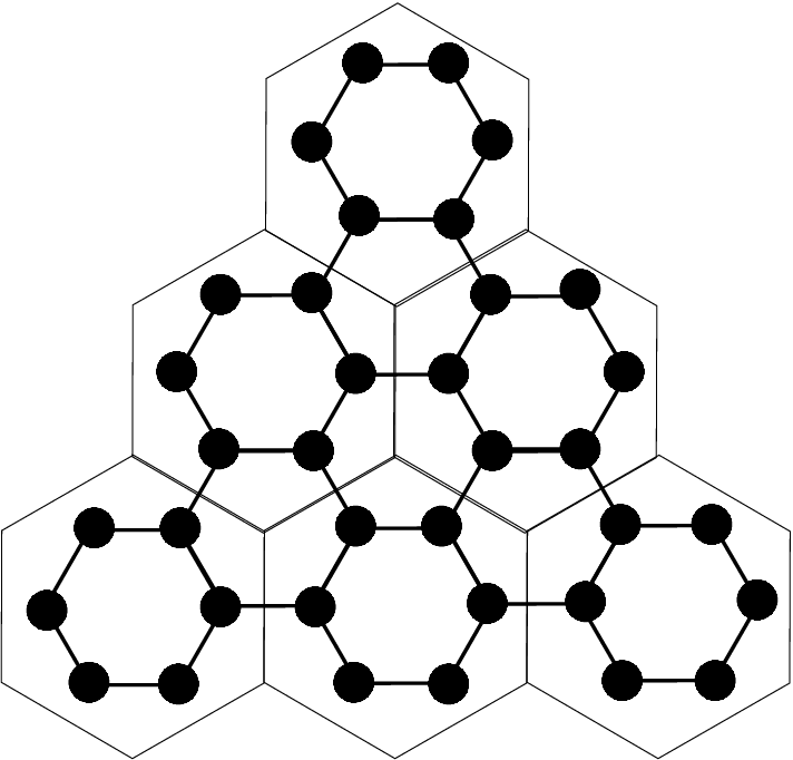
This formula can be derived if one splits the dot into $N_{0}(N_{0}+1)/2$ aromatic rings, with six atoms each (see Fig. 5).

The atoms at the edges of the dot are special for they have only two nearest neighbors, unlike atoms in the “bulk” of the dot, which have three neighbors. As a result, the Schrödinger equations, Eq. (33) and Eq. (34), for the atoms at the edges have to be modified. It is not always convenient to work with such formalism. A simpler approach is used in Ref. [9, 10]. In those works it is pointed out that one may add an extra row of carbon atoms at the armchair edges (‘auxiliary’ atoms, shown as hatched circles in Fig. 4) and demand the wave function to vanish on these ‘atoms’. Then for a physical (not ‘auxiliary’) atom at the edge we do not have to amend Eqs. (33) and (34) explicitly. Indeed, the absent neighbor (now represented by the ‘auxiliary’ atom) does not contribute to these equations, since the wave function vanishes on the ‘auxiliary’ atoms.

The addition of the extra row of ‘auxiliary’ atoms slightly increases the effective size of the dot. It is helpful to introduce the following notation:

$\displaystyle L=L_{0}+3a_{0}=3Na_{0},{\rm\ where\ }N=N_{0}+1.$

(47)

Although $L$ and $N$ are trivially related to $L_{0}$ and $N_{0}$, it is convenient to define these quantities explicitly for they are heavily used in the calculations below.

Consider now the wave function:

$\displaystyle\Psi_{{\bf R}\pm}=\sum_{\alpha=1}^{6}(-1)^{\alpha+1}\Psi_{{\bf k}_{\alpha}\pm}\exp(-i{\bf k}_{\alpha}{\bf R}),$

(48)

where ${\bf k}_{\alpha}$ are members of a sextet. They are given in section II. Observe now that:

$\displaystyle\varepsilon_{{\bf k}_{1}\pm}=\varepsilon_{{\bf k}_{2}\pm}=\varepsilon_{{\bf k}_{3}\pm}=\varepsilon_{{\bf k}_{4}\pm}=\varepsilon_{{\bf k}_{5}\pm}=\varepsilon_{{\bf k}_{6}\pm}.$

(49)

This is a consequence of the graphene lattice symmetry. Therefore, the spinor $\Psi_{{\bf R}\pm}$ is a solution of Eqs. (33) and (34) with eigenvalue $\varepsilon_{{\bf k}_{1}\pm}$.

Further, the upper component of $\Psi_{{\bf R}\pm}$ coincides with $\psi({\bf R})$, Eq. (14). Thus, if ${\bf k}_{1}$ satisfies Eqs. (22) and (23), then $\psi^{\cal A}_{{\bf R}\pm}$ complies with the boundary condition. We remind the reader that the zero boundary conditions must be met at the effective edges of the TQD (on the ‘auxiliary’ atoms).

The lower component of $\Psi_{{\bf R}\pm}$ requires a more tedious consideration. It is equal to:

$\displaystyle\psi^{\cal B}_{{\bf R+{\bm{\delta}}}_{1}\pm}=\mp\sum_{\alpha}(-1)^{\alpha+1}\exp(-i\theta_{{\bf k}_{\alpha}})\exp(-i{\bf k}_{\alpha}{\bf R}).$

(50)

As Eq. (35) specifies, the argument of $\psi^{\cal B}$ is not ${\bf R}$, which belongs to sublattice ${\cal A}$, but rather the sum ${\bf R+{\bm{\delta}}}_{1}$, which belongs to sublattice ${\cal B}$ (recall that ${\bf R}$ is the coordinate of the two-atom unit cell, while ${\bf R+{\bm{\delta}}}_{1}$ is the physical location of the atom on sublattice ${\cal B}$). We must keep this in mind when formulating the following boundary conditions for $\psi^{\cal B}$:

	$\displaystyle\psi^{\cal B}_{{\bf R+{\bm{\delta}}}_{1}\pm}$	$\displaystyle=$	$\displaystyle 0,{\rm\ if\ }y=0;$		(51)
	$\displaystyle\psi^{\cal B}_{{\bf R+{\bm{\delta}}}_{1}\pm}$	$\displaystyle=$	$\displaystyle 0,{\rm\ if\ }{\bf R+{\bm{\delta}}}_{1}={\bf u}s,$		(53)
			$\displaystyle{\rm\ where\ }{\bf u}=\frac{1}{2}(1,\sqrt{3}),s=(3l-1)a_{0};$
	$\displaystyle\psi^{\cal B}_{{\bf R+{\bm{\delta}}}_{1}\pm}$	$\displaystyle=$	$\displaystyle 0,{\rm\ if\ }{\bf R+{\bm{\delta}}}_{1}={\bf r}_{0}+{\bf v}s^{\prime},$		(55)
			$\displaystyle{\rm\ where\ }s^{\prime}=(3l+1)a_{0}.$

Here $l$ is an integer; ${\bf r}_{0}$ and ${\bf v}$ are defined in Eq. (16).

The first condition, Eq. (51), is fulfilled automatically. Indeed, it is easy to check that $\exp(-i\theta_{\bf k})$ is independent of the sign of $k_{y}$. Thus

	$\displaystyle\exp(-i\theta_{{\bf k}_{1}})\exp(-i{\bf k}_{1}{\bf R})-\exp(-i\theta_{{\bf k}_{2}})\exp(-i{\bf k}_{2}{\bf R})$		(56)
	$\displaystyle=-2i\exp(-i\theta_{{\bf k}_{1}})\exp(-ik_{x}x)\sin(k_{y}y),$

vanishes, when $y=0$. The same holds true for the sum of the third and sixth terms, as well as for the sum of the fourth and fifth terms.

Let us now show that Eq. (53) is valid. It is convenient to rewrite Eq. (50) as:

	$\displaystyle\psi^{\cal B}_{{\bf R+\delta}_{1}\pm}=\mp\sum_{\alpha}(-1)^{\alpha+1}\exp(-i\theta_{{\bf k}_{\alpha}}-ik_{x\alpha}a_{0})$		(57)
	$\displaystyle\times\exp\left[-i{\bf k}_{\alpha}({\bf R}+{\bm{\delta}}_{1})\right].$

When ${\bf R+{\bm{\delta}}}_{1}={\bf u}s$, we have:

	$\displaystyle\psi^{\cal B}_{{\bf R+\delta}_{1}\pm}=\mp\Big\{A\exp\left[-\frac{i}{2}(k_{x}+\sqrt{3}k_{y})s\right]$		(58)
	$\displaystyle+B\exp\left[-\frac{i}{2}(k_{x}-\sqrt{3}k_{y})s\right]+C\exp(ik_{x}s)\Big\},$

where

	$\displaystyle A=\exp(-i\theta_{{\bf k}_{1}}-ik_{x1}a_{0})-\exp(-i\theta_{{\bf k}_{6}}-ik_{x6}a_{0}),$		(59)
	$\displaystyle B=\exp(-i\theta_{{\bf k}_{5}}-ik_{x5}a_{0})-\exp(-i\theta_{{\bf k}_{2}}-ik_{x2}a_{0}),$		(60)
	$\displaystyle C=\exp(-i\theta_{{\bf k}_{3}}-ik_{x3}a_{0})-\exp(-i\theta_{{\bf k}_{4}}-ik_{x4}a_{0}).$		(61)

Note that the equation for $A$ involves two wave vectors: ${\bf k}_{1}$ and ${\bf k}_{6}$. They enter together because ${\bf u}{\bf k}_{1}={\bf u}{\bf k}_{6}$. For the same reason the vectors ${\bf k}_{2}$ and ${\bf k}_{5}$ appear in the equation for $B$, and the vectors ${\bf k}_{3}$ and ${\bf k}_{4}$ are part of the equation for $C$. A similar structure was already observed above, see the discussion after Eq. (17).

It is easy to check that

	$\displaystyle\exp(-i\theta_{{\bf k}_{6}})=\exp\left(-\frac{3i}{2}k_{x}a_{0}+\frac{\sqrt{3}i}{2}k_{y}a_{0}\right)$		(62)
	$\displaystyle\times\exp(-i\theta_{{\bf k}_{1}}).$

To prove this identity one has to use Eqs. (38) and (40), and the fact that $|t_{\bf k}|=\varepsilon_{{\bf k}+}$ is the same for all members of the sextet, see Eq. (49). Consequently

	$\displaystyle A=\exp(-i\theta_{{\bf k}_{1}}-ik_{x1}a_{0})\qquad\qquad$		(63)
	$\displaystyle\times\left\{1-\exp\left[-ia_{0}\left(\frac{3}{2}k_{x}-\frac{\sqrt{3}}{2}k_{y}-k_{x1}+k_{x6}\right)\right]\right\}.$

Using the definitions of ${\bf k}_{1}$ and ${\bf k}_{6}$ we can write:

$\displaystyle-k_{x1}+k_{x6}=-\frac{3}{2}k_{x}+\frac{\sqrt{3}}{2}k_{y}.$

(64)

Thus, the argument of the exponential in Eq. (63) vanishes, and the coefficient $A$ vanishes as a result. In a similar fashion, it is possible to prove that $B$ and $C$ are equal to zero.

Lastly, we need to demonstrate that $\psi^{\cal B}$ satisfies Eq. (55). When ${\bf R+{\bm{\delta}}}_{1}={\bf r}_{0}+{\bf v}s^{\prime}$, we use Eq. (57) to obtain:

	$\displaystyle\psi^{\cal B}_{{\bf R+\delta}_{1}\pm}=\mp\Big\{A\exp\left[\frac{i}{2}(k_{x}-\sqrt{3}k_{y})s^{\prime}\right]$		(65)
	$\displaystyle+B\exp\left[\frac{i}{2}(k_{x}+\sqrt{3}k_{y})s^{\prime}\right]+C\exp(-ik_{x}s^{\prime})\Big\},$

with the coefficients:

	$\displaystyle A$	$\displaystyle=$	$\displaystyle\exp[-i\theta_{{\bf k}_{1}}-ik_{x}(L+a_{0})]$		(66)
		$\displaystyle-$	$\displaystyle\exp[-i\theta_{{\bf k}_{4}}+\frac{i}{2}(k_{x}+\sqrt{3}k_{y})(L+a_{0})],$
	$\displaystyle B$	$\displaystyle=$	$\displaystyle-\exp[-i\theta_{{\bf k}_{2}}-ik_{x}(L+a_{0})]$		(67)
		$\displaystyle+$	$\displaystyle\exp[-i\theta_{{\bf k}_{3}}+\frac{i}{2}(k_{x}-\sqrt{3}k_{y})(L+a_{0})],$
	$\displaystyle C$	$\displaystyle=$	$\displaystyle\exp[-i\theta_{{\bf k}_{5}}+\frac{i}{2}(k_{x}+\sqrt{3}k_{y})(L+a_{0})]$		(68)
		$\displaystyle-$	$\displaystyle\exp[-i\theta_{{\bf k}_{6}}+\frac{i}{2}(k_{x}-\sqrt{3}k_{y})(L+a_{0})].$

Using the relation:

	$\displaystyle\exp(-i\theta_{{\bf k}_{4}})=\exp\left(-\frac{3i}{2}k_{x}a_{0}-\frac{\sqrt{3}i}{2}k_{y}a_{0}\right)$		(69)
	$\displaystyle\times\exp(-i\theta_{{\bf k}_{1}}),$

which is similar to Eq. (62) and is derived analogously, we show that:

	$\displaystyle A$	$\displaystyle=$	$\displaystyle\exp[-i\theta_{{\bf k}_{1}}-ik_{x}(L+a_{0})]$		(70)
		$\displaystyle\times$	$\displaystyle\left\{1-\exp\left[iL\left(\frac{3}{2}k_{x}+\frac{\sqrt{3}}{2}k_{y}\right)\right]\right\}.$

From here we obtain:

$\displaystyle A=0\;\Leftrightarrow\;L\left(\frac{3}{2}k_{x}+\frac{\sqrt{3}}{2}k_{y}\right)=2\pi n.$

(71)

For the coefficient $B$, the following expression holds:

	$\displaystyle B$	$\displaystyle=$	$\displaystyle\exp[-i\theta_{{\bf k}_{2}}-ik_{x}(L+a_{0})]$		(72)
		$\displaystyle\times$	$\displaystyle\left\{-1+\exp\left[iL\left(\frac{3}{2}k_{x}-\frac{\sqrt{3}}{2}k_{y}\right)\right]\right\}.$

Deriving Eq. (72), we use the relation:

	$\displaystyle\exp(-i\theta_{{\bf k}_{3}})=\exp\left(-\frac{3i}{2}k_{x}a_{0}+\frac{\sqrt{3}i}{2}k_{y}a_{0}\right)$		(73)
	$\displaystyle\times\exp(-i\theta_{{\bf k}_{2}}).$

Coefficient $B$ vanishes when

$\displaystyle L\left(\frac{3}{2}k_{x}-\frac{\sqrt{3}}{2}k_{y}\right)=-2\pi m.$

(74)

Coefficient $C$ vanishes automatically, when both Eq. (71) and Eq. (74) hold.

Combining Eq. (71) and Eq. (74) we derive the quantization condition:

	$\displaystyle{\bf k}_{1}={\bf k}^{n,m},$		(75)
	$\displaystyle{\rm where\ }{\bf k}^{n,m}=n{\bf K}_{1}+m{\bf K}_{2},$		(76)
	$\displaystyle{\bf K}_{1,2}=\left(\pm\frac{2\pi}{9Na_{0}},\frac{2\pi}{3\sqrt{3}Na_{0}}\right).$		(77)

which is equivalent to Eqs. (22) and (23) with $L$ given by Eq. (47). The symbol $\Psi_{\bf R}^{n,m}$ is used below to denote the wave function with ${\bf k}_{1}={\bf k}^{n,m}$.

Thus, we demonstrate that the wave function Eq. (48) with momentum quantized according to Eq. (75) satisfies the Schrödinger equations (33) and (34) on a TQD with armchair edges.

In this section we study the most elementary properties of the Schrödinger equation solution $\Psi_{\bf R}^{n,m}$.

References

• [1] A.H. Castro Neto, F. Guinea, N.M.R. Peres, K.S. Novoselov, and A.K. Geim, Rev. Mod. Phys., 81, 109 (2009);
• [2] A. Cresti, N. Nemec, B. Biel, G. Niebler, F. Triozon, G. Cuniberti, and S. Roche, Nano Research, 1, 361, (2008).
• [3] A.K. Geim, Science 324, 1530 (2009).
• [4] E.g., T.G. Pedersen, C. Flindt, J. Pedersen, N.A. Mortensen, A.P. Jauho, K. Pedersen, Phys. Rev. Lett. 100, 136804 (2008); A. Matulis, F.M. Peeters, Phys. Rev. B77, 115423 (2008); J.M. Pereira, Jr., P. Vasilopoulos, and F.M. Peeters, Nano Lett., 7, 946 (2007); K.A. Ritter and J.W. Lyding, Nat. Mat. 8, 235, (2009).
• [5] E.g., E.V. Castro, N.M.R. Peres, J.M.B. Lopes dos Santos, A.H. Castro Neto, F. Guinea, Phys. Rev. Lett. 100, 026802 (2008); K. Kechedzhi, V.I. Falko, E. McCann, B.L. Altshuler, Phys. Rev. Lett. 98, 176806 (2007);
• [6] E.g., L. Yang, C.-H. Park, Y.-W. Son, M. L. Cohen, and S. G. Louie, Phys. Rev. Lett. 99, 186801 (2007); K. Nakada and M. Fujita, G. Dresselhaus, and M. S. Dresselhaus, Phys. Rev. B 54 17954 (1996); C. T. White, J. Li, D. Gunlycke, and J. W. Mintmire, Nano Lett. 7, 825 (2007); A.V. Nikolaev, A.V. Bibikov, A.V. Avdeenkov, I.V. Bodrenko, and E.V. Tkalya, Phys. Rev. B 79, 045418, (2009);
• [7] M. Fujita, M. Igami, and K. Nakada, J. Phys. Soc. Jpn. 66, 1864, (1997);
• [8] Y.-W. Son, M. L. Cohen, and S. G. Louie, Phys. Rev. Lett. 97, 216803, (2006).
• [9] D. Gunlycke and C.T. White, Phys. Rev. B 77, 115116, (2008).
• [10] A.V. Rozhkov, S.S. Savel’ev, F. Nori, Phys. Rev. B 79, 125420, (2009).
• [11] E.g., J.M. Pereira Jr., F.M. Peeters, and P. Vasilopoulos, Phys. Rev. B 75, 125433 (2007); Ch. Bai, X. Zhang, Phys. Rev. B, 76, 075430 (2007); J.R. Williams, L. DiCarlo, C.M. Marcus, Science, 317, 638 (2007); L. DiCarlo, J.R. Williams, Y. Zhang, D.T. McClure, C.M. Marcus, Phys. Rev. Lett., 100, 156801 (2008); C.-H. Park, Y.-W. Son, L. Yang, M.L. Cohen, and S.G. Louie, Phys. Rev. Lett., 103, 046808 (2009); L. Brey, H.A. Fertig, Phys. Rev. Lett. 103, 046809 (2009); V.A. Yampol’skii, S. Savel’ev, F. Nori, New J. Phys., 10, 053024 (2007); Y.P. Bliokh, V. Freilikher, S. Savel’ev, F. Nori, Phys. Rev. B, 79, 075123 (2009); V.A. Yampol’skii, S.S. Apostolov, Z.A. Maizelis, A. Levchenko, F. Nori, arXiv:0903.0078 (unpublished); Y.P. Bliokh, V. Freilikher, and F. Nori, arXiv:0910.3106 (unpublished).
• [12] J. Fernandez-Rossier, J. J. Palacios, Phys. Rev. Lett. 99, 177204 (2007); M. Ezawa, Phys. Rev. B 76, 245415, (2007); O. Hod, V. Barone, and G.E. Scuseria, Phys. Rev. B 77, 035411, (2008); C. Tang, W. Yan, Y. Zheng, G. Li, and L. Li, Nanotech., 19, 435401 (2008); Z.Z. Zhang and K. Chang, F.M. Peeters, Phys. Rev. B 77, 235411, (2008); M. Ezawa, EPJB, 67, 543, (2009); D.A. Bahamon, A.L.C. Pereira, and P.A. Schulz, Phys. Rev. B 79, 125414, (2009); S. Schenez, K. Ensslin, M. Sigrist, and T. Ihn, Phys. Rev. B 78, 195427, (2008).
• [13] H.P. Heiskanen, M. Manninen, and J. Akola, New J. of Phys., 10, 103015, (2008); M. Manninen, H. P. Heiskanen, J. Akola, Eur. Phys. J. D, 52, 143, (2009).
• [14] J. Akola, H.P. Heiskanen, and M. Manninen, Phys. Rev. B 77, 193410, (2008).
• [15] P. Potasz, A. D. Güçlü, P. Hawrylak, arXiv:0910.4121v1 (unpublished).
• [16] H.R. Krishnamurthy, H.S. Mani and H.C. Verma, J. Phys. A: Math. Gen., 15, 2131, (1982); M. A. Doncheski, S. Heppelmann, R. W. Robinett, D. C. Tussey, Am. J. Phys. 71, 541 (2003).
• [17] L.D. Landau and L.M. Lifshitz, “Quantum Mechanics (Non-Relativistic Theory)” (Butterworth-Heinemann, 1981).