HU-EP-09/60
LU-ITP 2009/002
Two-point functions of quenched lattice QCD
in Numerical Stochastic Perturbation Theory.
(I) The ghost propagator in Landau gauge
Abstract
This is the first of a series of two papers on the perturbative computation of the ghost and gluon propagators in Lattice Gauge Theory. Our final aim is to eventually compare with results from lattice simulations in order to enlight the genuinely non-perturbative content of the latter. By means of Numerical Stochastic Perturbation Theory we compute the ghost propagator in Landau gauge up to three loops. We present results in the infinite volume and limits, based on a general strategy that we discuss in detail.
1 Introduction
The identification of confinement mechanisms is a challenge for Lattice QCD [1, 2, 3]. This requires to single out observables which both capture the relevant physical content and are in the end suitable for numerical simulations, so that a non-perturbative investigation becomes possible. The gluon and the ghost propagators with their momentum dependence are believed to encode specific features and mechanisms of a confining theory [2], which can be studied once a gauge is fixed. Apart from the non-unique asymptotic infrared behavior, which – if calculated in lattice simulations – realizes the so-called decoupling solution instead of the scaling solution (see Refs. [4, 5, 6]) of the Schwinger-Dyson and Functional Renormalization Group [7] approaches 11 1 The latter solution is preferred in view of the Gribov-Zwanziger [8, 9] and Kugo-Ojima [10, 11] confinement scenarios. The conflict with lattice calculations has given rise to a controversy about the (in)dispensability of having a BRST-invariant lattice gauge-fixing prescription. It is argued to be possible [12] although still lacking. This interesting development is probably irrelevant for the aspects discussed below., in these functions the onset of non-perturbative effects is generally agreed to be associated with the following two aspects: the coupling to local condensates [13] and to localized vacuum excitations like vortices [14, 15]. In order to effectively face the genuine non-perturbative effects, it is desirable to have for reference an understanding of the perturbative behavior of these gauge-dependent functions in higher than one-loop order.
Such a program cannot evade a well-known practical problem: Lattice Perturbation Theory (LPT) is much more involved compared to its continuum QCD counterpart. The complexity of the diagrammatic approaches rapidly increases beyond the one-loop approximation [16]. By now, only a limited number of results up to two-loop accuracy has been obtained. As an effective alternative to diagrammatic LPT a numerical tool has been proposed by the Parma group in [17]. The method is a quite direct numerical implementation of Stochastic Perturbation Theory, which in turn comes as one of the two main applications of the ideas of Stochastic Quantization, the other being the use of Langevin dynamics as an alternative to standard Monte Carlo techniques [18, 19]. This numerical tool for LPT goes under the name of Numerical Stochastic Perturbation Theory (NSPT) and has been reviewed in [20].
In a joined effort we started a new field of application for NSPT based on our respective interests in LPT (Leipzig), NSPT (Parma) and Monte Carlo studies of gluon and ghost propagators (Berlin). First results have been presented at Lattice 2007 [21, 22], Lattice 2008 [23], Confinement8 [24] and at Lattice 2009 [25]. The present paper is the first of a series of two. While this paper is concentrated on the ghost propagator, the forthcoming one will present the results for the gluon propagator.
One of our main goals is to provide results for the comparison of higher-loop calculations of perturbative contributions with the results of lattice Monte Carlo calculations of the main propagators in QCD on finite size lattices. The other goal consists in determining higher loop contributions to the logarithmically divergent perturbative ghost propagator in momentum space including non-logarithmic contributions to good precision. The present work also aims at a further check on the precision of the method by comparison to known one-loop results from LPT. In order to proceed to two- and higher-loop results in the infinite volume limit, peculiar emphasis will be put on the control of finite size effects. We want to stress that our results have been obtained from two completely independent sources: while strategies have been extensively discussed, the actual implementation of Parma and Leipzig NSPT codes are completely independent of each other, thus providing a stronger check on numerical results.
The paper is organized as follows. In Sect. 2 we present selected elements of NSPT which are relevant for the case at hand, in particular the issue of performing a NSPT computation in a fixed gauge, i.e. the minimal Landau gauge. Sect. 3 focuses on the observables we will be concerned with, while Sect. 4 summarizes known analytic results for the perturbative ghost propagator up to three-loop order and their relation to the unknown non-logarithmic coefficients we want to determine. In the following section we present the technical details of practicing NSPT. Finally we collect our results in Sect. 6 and briefly discuss a comparison to Monte Carlo data.
2 Landau gauge fixing in NSPT
The basis of Stochastic Quantization is the (stochastic) time evolution of fields driven by the Langevin equation. In the case of a lattice gauge theory the Langevin equation for the matrix located at the link between lattice sites and reads
| (1) |
is the (stochastic) Langevin time. The so-called drift term is given by the equations of motion derived from the Euclidean gauge action : they are written in terms of the differential operator , which is a left Lie derivative. The () are the generators in the fundamental representation. In our case we will have and the gauge action is the Wilson plaquette action.
The key issue of Stochastic Quantization is that in the limit of large expectation values with respect to the noise converge to expectation values with respect to the QFT functional integral, i.e. the distribution of the gauge fields converges to the Gibbs measure . In any numerical approach (and this applies to our case), however, the Langevin equation is not solved for continuous time. One needs to discretize time as a sequence , with running step number . Therefore, in order to extract correct physical information, one needs to perform the double extrapolation and . For the numerical solution of the Langevin equation we adhere to a peculiar version of the Euler scheme that guarantees all the link matrices to stay in the group manifold:
| (2) | |||||
| (3) |
In matrix form and at finite , the components of are subject to the mutual correlations ()
| (4) |
and (integer) denote here Langevin time steps. The noise is white, meaning that different time steps are uncorrelated.
The usual path from Stochastic Quantization to Stochastic Perturbation Theory would go through trading the differential form of Langevin equation for its integral equation counterpart in a Green function formalism, which is easy to solve in a perturbative scheme. NSPT remains instead in a differential formulation. For the case of Lattice Gauge Theories we rewrite each link matrix as an expansion in the bare coupling constant . Since , the expansion reads
| (5) |
Provided one rescales the time step to , the expansion converts the Langevin equation (2) into a system of simultaneous updates in terms of the expansion coefficients (5) of and of similar expansion coefficients for the force in Eq. (3). While the random noise enters only the lowest order equation, higher orders are stochastic by the noise propagating from lower order to higher order terms. The system can be truncated according to the maximal order of the gauge field one is interested in.
In a notation which is common in Lattice Perturbation Theory we can relate the (antihermitean) vector potential to the link matrices via
| (6) |
An expansion similar to (5) exists for that potential taking values in the algebra ,
| (7) |
We observe that unitarity of has a counterpart in the antihermiticity and tracelessness of all orders of :
| (8) |
As we will see, the definition of the ghost propagator will in a sense be based on the expansion in the algebra.
We finally remark that whenever we speak about contributions of some order to an observable this has to be understood as an expansion
| (9) |
and constructed by comparison to coefficients of .
We now come to the main point of how to perform a gauge-fixed NSPT computation, in the case at hand in Landau gauge. A key issue of the standard (in other words, non-perturbative) Langevin equation for LGT is the non-necessity of fixing a gauge. In short: the drift term in Langevin equation is equal to the lattice equations of motion (put equal zero there). As a consequence, longitudinal degrees of freedom undergo an unbounded diffusion, but the group manifold is compact and hence no divergence shows up. Such a situation is no longer true in NSPT. This is quite obvious in the algebra: the diffusion of the longitudinal component of the fields is unbounded and hence their norms diverge in stochastic time. We stress that gauge-invariant quantities are in principle not affected by these divergences, but this is no advantage: since norms are diverging one runs eventually into trouble by lack of accuracy. We also remark that this is true regardless of the choice of either expansion (7) or (5): perturbation theory implies decompactification in any case.
A solution comes along the lines suggested in [26]: fixing (to some precision) the gauge is going to fix the problem and this goes under the name of Stochastic Gauge Fixing. We adhere here to the recipe of [20]. The Langevin evolution steps are interwoven with gauge transformations
| (10) |
The main requirement for is quite obvious: gauge transformations should be expanded in the coupling as well and the leading order should not affect the background vacuum around which the solution to Langevin equation is expanded (the trivial vacuum, in the case at hand). A convenient solution comes with the choice
| (11) |
In general the action of the left/right lattice derivative on a function defined on site is given by
| (12) |
The action of the left lattice derivative on the vector potential defined on midpoints of the links is defined as
| (13) |
The resulting divergence is mapped to site . We will come back to this choice: the iteration of this gauge transformation would drive the field configuration to the Landau gauge.
With respect to Stochastic Gauge Fixing, it suffices here to point out that one step of (10) using (11) interwoven with the Langevin step (2) is enough to keep fluctuations under control provided that is chosen of order . The rationale for this is the essence of Stochastic Gauge Fixing: any new drift term in the Langevin equation which amounts to a local gauge transformation does not affect the asymptotic distribution of gauge invariant quantities, while it can provide a restoring force in the non-gauge-invariant sector. The differential (finite difference, actually) operator present in (11) makes it clear that zero modes are completely unaffected up to this point. Their divergences are still present. We take the simplest prescription of subtracting zero modes at every order.
One can actually do more than this and perform a gauge-fixed NSPT computation in the case of covariant gauges. The interested reader is referred to [27]. The key issue is that one can rewrite the functional integral in the Faddeev-Popov formalism, which merely results in a different form of the gauge action (an effective action, one would say). Without entering into details, in this context it is worth making two points. First, there is no need for the introduction of ghost fields: one simply faces an extra contribution to the action in the form , being the Faddeev-Popov operator we will be concerned with in the following. Second, for the Landau gauge the procedure is of little help, since the other extra piece in the action is the gauge fixing action , with being the covariant gauge parameter, which is zero in this case.
The failure of the general covariant gauge NSPT procedure has anyway a counterpart: as a limit case of covariant gauges, the Landau gauge
| (14) |
is related to an extremum of the norm of the field, and there is a well-known iterative procedure to reach such an extremum. The basic step is (11), i.e. the gauge transformation that we also use for Stochastic Gauge Fixing. The iteration stops when, for all orders , the summed-up quadratic violations of (14) vanish within double precision ( is the lattice volume),
| (15) |
Iterating (10) with (11) is actually not very efficient, since it suffers from critical slowing down due to the low modes, which becomes more and more severe as the lattice size increases.
An effective solution to this problem is also well-known and goes through Fourier acceleration as introduced in [28]. In NSPT one makes use of the expanded variant of the gauge transformation
| (16) |
in order to achieve the minimal Landau gauge. denotes the Fourier transformation from discrete to momentum space and its inverse. The gauge transformation (16) applied locally is actually not local in the sense of (11). The driving force, the divergence of the gauge potential, is non-locally smeared with a low-pass filter that attenuates the higher Fourier components of by a factor . Here is a non-zero eigenvalue of the free field lattice Laplacian, and its maximal value on a periodic lattice in all directions is . While we notice that the volume-independent optimal parameter for the case of periodic boundary conditions in all directions is found for this perturbative Landau gauge fixing to be , we also point out that Fourier acceleration also works if one takes the plain lattice momenta (which in the following we will reference as ) instead of .
This is a good point to pin down some notations for lattice momenta. In the following we will reserve the latin letter to denote , the integer 4-tuples , while plain lattice momenta will be denoted by
| (17) |
Here is the lattice size in direction and the reference to lattice spacing can be made explicit: . In our case lattices will be symmetric, i.e. and . According to the two most popular conventions, or . The eigenvalues of the free Laplacian are
| (18) |
where for each direction separately
| (19) |
3 The lattice ghost propagator
The ghost propagator is nothing but the inverse of the Faddeev-Popov operator . We start our discussion in the continuum, where – in the case of covariant gauges – the Faddeev-Popov (FP) operator reads
| (20) |
is the covariant derivative, emerging from the response of the gauge field to an infinitesimal gauge transformation. is diagonal in the (adjoint) color space ()
| (21) |
As an average over field configurations , it is translationally invariant
| (22) |
In Landau gauge, because , we can reverse the order of and ,
| (23) |
To obtain the form of the FP operator on the lattice one closely mimics the steps one goes through in the continuum. The lattice form of that operator is nevertheless much more involved, since the response of the Lie-algebra field to a gauge transformation does not have a closed form. In perturbation theory there is no logical obstruction, anyway: at any given order the lattice counterpart of the covariant derivative can be pinned down [29, 30] and all in all the FP operator reads
| (24) |
Here we denote by the lattice counterpart of the covariant derivative, indicating a dependence on , even if this dependence is through a perturbative expansion. This results in a dependence on the adjoint representation of the Lie-algebra field
| (25) |
The is the adjoint representation of the lattice gauge field (, antihermitean)
| (26) |
the fundamental representation being given by ():
| (27) |
The ghost propagator in momentum space can in principle be obtained by Fourier transformation in each lattice configuration , taking the translational invariance into account:
| (28) |
with the scalar product . Given the color-diagonal form, one is interested in the scalar function defined by the adjoint trace
| (29) |
Due to its eight trivial zero eigenvalues (corresponding to global gauge transformations) the inverse needs to be defined with care. Since one is interested in non-zero momenta , this means that one is automatically restricted to a subspace orthogonal to the space spanned by the (space-time constant) zero modes of the Faddeev-Popov operator.
For an individual configuration, the inverse of the FP operator is not translationally invariant and hence (28) is not so useful. The way out is quite standard and goes through the inversion of on a delta source in momentum space, i.e. a plane wave source in real space:
| (30) |
As in standard non-perturbative applications, the issue is inverting the relevant operator on a source, but things are actually a lot easier in NSPT. The matrix can simply be considered as expanded using the expansion of the gauge fields :
| (31) |
Then the inverse of will also obtained as a power series
| (32) |
One easily finds [20] a recursive way to obtain the higher orders of :
| (33) | |||||
It is worth pointing out that the computation proceeds back and forth from position to momentum space, since at any step the operators at hand are diagonal (or almost diagonal) in one of the two spaces.
This is the time to reintroduce perturbative (loop) indices: we denote the loop order of the ghost propagator as
| (34) |
Thus a real loop order of the ghost propagator corresponds to contributions with even powers , whereas contributions with odd powers would indicate a non-loop contribution which does not exist by construction in standard perturbation theory. Contributions related to these non-integer have to vanish numerically in NSPT for sufficiently large statistics.
Similar to the gluon propagator in the forthcoming paper, we present the various orders of the ghost dressing function (or “form factor”) in two forms:
| (35) |
The dressing function has to be calculated for each 4-momentum given by four integers – the momentum 4-tuple .
Two comments are in order for (35). First of all, the ’s are dimensionless quantities. Notice that in a numerical lattice simulation one does not have access to , but to the dimensionless quantity . Multiplying by - or - one obtains the corresponding (still dimensionless) - or - we will be concerned with in the following. Second, the second notation in (35) is chosen to remind that here the quantities are acting as the “physical” momenta.
4 Relation to standard Lattice Perturbation Theory
In the RI’-MOM scheme, the renormalized ghost dressing function is defined as
| (36) |
with the condition
| (37) |
Therefore, the ghost dressing function is just the ghost wave function renormalization constant at .
The general form of an operator/function in terms of the renormalized coupling 22 2 Note the additional factor compared to the “standard” definition. can be written as
| (38) |
Here gives the possible powers of the logarithms in loop order .
Using (36) and (37), we get the expansions
| (39) | |||||
| (40) | |||||
| (41) |
Since we measure the dressing function as an expansion in the lattice (inverse) coupling , we need the ghost wave function renormalization as an expansion in the lattice coupling :
| (42) |
From now we restrict ourselves to three-loop expressions in Landau gauge and in the quenched approximation. The logarithmic corrections are partly known from the anomalous dimension of the ghost field and the beta function and given as follows (compare e.g. [31])
| (43) | |||
| (44) | |||
| (45) | |||
The finite one-loop constant has been calculated from the ghost self-energy in standard infinite volume LPT [32] with the value
| (46) |
To our knowledge, the constants and were not known so far.
Taking into account the relation between the lattice coupling and the renormalized coupling in two-loop accuracy [33, 34, 35] (the function is scheme independent)
| (47) |
with
| (48) | |||
| (49) | |||
| (50) |
we get the coefficients of in (42) up to three loops
| (51) | |||
| (52) | |||
| (53) | |||
Using these numbers and the inverse lattice coupling we obtain the expression for the ghost dressing function to that order
| (54) |
with the one-loop coefficients
| (55) |
the two-loop coefficients
| (56) | |||||
and the three-loop coefficients
| (57) | |||||
Thus we conclude: the coefficients of the leading logarithmic contributions for a given order can be exclusively taken from continuum computations whereas non-leading log coefficients are already influenced by finite lattice constants from corresponding lower loop orders.
In general, these logarithmic terms are the relatively easy part of a diagrammatic perturbative computation, while getting the finite constants is the big effort. In NSPT it is just the other way around. As it will be clear in Section 5.2, telling which is which in the measured ghost dressing function at each loop requires a fitting procedure: fitting a logarithmic term would actually require a terrific precision. As a consequence, we have just stated from the very beginning the (modest) attitude of not even trying to extract anomalous dimensions from our NSPT computations. On the contrary, we have to assume that the coefficients in front of the logarithms are known. Assuming that a continuum calculation has been performed up to a given loop order defines the maximum accuracy and the maximal loop number which we can reach in a lattice NSPT computation.
We have to check that NSPT in the limits (or ) and reproduces the constant from the one-loop result. After that we may proceed to determine from the two-loop measurements the unknown and, therefore, . Knowing that number, we are in the position to fix the coefficients of all non-leading logarithmic contributions in the three-loop expression and to estimate the constant or from the three-loop measurements.
5 The practice of NSPT simulations
5.1 Statistics and extrapolation to zero Langevin step
Choosing a maximal loop expansion order and solving the coupled system of equations for the gauge links and the gauge potentials simultaneously, one generates a sequence of these fields for all perturbative orders . Such sequences — representing Langevin time trajectories — are generated for different finite Langevin time steps and different lattices sizes, i.e. different .
From the perturbative fields at finite we construct the observable of interest, in our case the ghost dressing function for each chosen set of lattice momenta and average it over the used configurations within a Langevin time trajectory. It is expected that the autocorrelation time for the observable is extending over subsequent configurations and increases with decreasing . As a reasonable compromise between computer time and autocorrelation we have measured the ghost propagator using a sequence of configurations separated by 50 Langevin steps. Before measuring, Landau gauge has to be obtained on each configuration by satisfying (15) to high precision. To further increase the statistics, we have generated several different trajectories for a given and .
Since the ghost propagator has to be calculated for each individual momentum 4-tuple and the number of 4-tuples rapidly increases with the lattice size we have restricted ourselves to a certain set of momentum 4-tuples for our periodic symmetric lattice. We have chosen a cylindrical cut similar to Monte Carlo measurements such that the individual momentum components do not differ too strongly from each other. The direction of that 4-vector is chosen nearly along a lattice 4-volume diagonal. In a 4-tuple we have chosen the ordered integers modulo lattice size not to differ by more than one unit and have assumed a maximal difference .
During the Langevin evolution we treated all 4-tuples leading to non-identical measurements as independent ones. This led in our particular realization to 4-tuples 33 3 The described choice corresponds to the Leipzig code, in the Parma code not all of the highest momenta have been measured. for which we have measured the propagator. After obtaining the Langevin time averages we further averaged the propagator over 4-tuples which were equivalent due to lattice symmetries and ended up with the following set of inequivalent momentum 4-tuples for our lattices chosen with even site numbers used in the further analysis:
| (58) | |||
Choosing as example , out of originally chosen 108 4-tuples we get 25 inequivalent 4-tuples for which the propagator has been measured. A final average has been performed on the results from different trajectories.
| 1 | 2 | 1 | 2 | 1 | 2 | 1 | 2 | 1 | 2 | 1 | 2 | |
|---|---|---|---|---|---|---|---|---|---|---|---|---|
| loop | loop | loop | loop | loop | loop | |||||||
| 0.010 | 2500 | 2000 | 1800 | 1000 | 1200 | 864 | 1250 | 822 | 800 | 384 | 57 | 57 |
| 0.020 | 1750 | 1500 | 1250 | 1000 | 900 | 850 | 750 | 650 | 600 | 241 | 43 | 43 |
| 0.030 | 1100 | 1000 | 900 | 750 | 750 | 778 | 650 | 573 | 373 | 262 | 20 | 20 |
| 0.050 | 1100 | 1000 | 900 | 900 | 750 | 700 | 650 | 650 | 284 | 259 | 39 | 39 |
| 0.070 | 1100 | 1000 | 850 | 750 | 700 | 770 | 650 | 591 | 259 | 192 | 40 | 40 |
| 0.010, all loops | 990 | 676 | 1214 | 735 |
| 0.015, all loops | 0 | 0 | 1025 | 614 |
| 0.020, all loops | 753 | 620 | 968 | 565 |
| 0.030, all loops | 508 | 438 | 0 | 0 |
| 0.040, all loops | 0 | 0 | 539 | 369 |
| 0.050, all loops | 465 | 0 | 0 | 0 |
| 0.070, all loops | 442 | 301 | 0 | 0 |
we present our collected statistics for different Langevin steps and lattice volumes from the Leipzig and Parma code, respectively. Note that the Leipzig data contain only measurements up to two-loops (). Combining the measurements from all sources we have rather accurate data of the perturbative propagator at each momentum 4-tuple.
The behavior of the different orders of the dressing function is shown in Figure 1 for loop numbers and the non-loop contribution vs. at different volumes and fixed Langevin step size :
 |
 |
We note that the dressing function for the power , which is not a loop contribution 44 4 By construction of the FP operator the contribution is zero in NSPT., vanishes to a good accuracy for each individual lattice momentum 4-tuple after averaging over the configurations. This vanishing has to happen already at non-zero . In general, the behavior in the infrared (small lattice momenta) is a bit more noisy. For a finite number of measurements the eventually still non-zero non-loop contribution for some given 4-tuple is by several orders of magnitudes smaller compared to the “neighboring” -th and -th loop contributions.
Now we are in the position to perform the extrapolation to zero Langevin step for the ghost dressing function at each individual momentum 4-tuple from the available finite measurements at fixed lattice size. Since the Langevin system is solved in the Euler scheme in which pieces of are neglected, we fit the extrapolation of each order of the ghost dressing function to zero Langevin step by an ansatz of the form . The fit result is a function of the lattice momentum 4-tuple and depends on the lattice size. For most of the cases we used 5 different values, for the largest volume we had 7 Langevin steps for one- and two-loop and 4 such steps for the three-loop extrapolation.
The extrapolation to zero Langevin step is shown for momentum 4-tuples at and at in Figures 2 and 3, respectively.
 |
 |
 |
 |
 |
 |
In Figures 4 we show the extrapolation of the one- and two-loop contributions to zero Langevin step for .
 |
 |
The remaining volume dependence of individual loops contributions vs. at zero Langevin step is shown in Figure 5 for two-loop and three-loop dressing functions using some of the lattice volumes.
 |
 |
One of the aims of this project is to provide referential perturbative results for finite lattices and for lattice momenta without any restriction. For this purpose, no further extrapolation is necessary. An exhaustive comparison with Monte Carlo results is not attempted in this paper.
To reproduce LPT results in the infinite-volume limit at vanishing lattice spacing, however, different lattice sizes have to be studied in parallel as explained in the following.
5.2 Fitting the data
Our aim is to extract the finite constants for loop order in the perturbative expansion of the lattice ghost dressing function (54) in infinite volume and in the continuum limit as accurate as possible. As pointed out in section 4, at any loop, a computation would yield a sum of a finite contribution plus logarithmic terms. To be definite, we recall that at one-loop order one gets
| (59) |
with the known coefficient given in (55) and similar expressions for higher loops. In general, at loop order one gets terms up to power , and all logarithmic contributions arise from anomalous dimensions and the beta function. Given what is known in the RI’-MOM scheme, in our present computation we can aim at three loops. In particular, reproducing the known one-loop lattice constant is an obvious check for our NSPT results. However, any NSPT computation is performed at both finite lattice spacing and finite lattice size.
Let us first of all discuss the influence of the finite lattice spacing. Any lattice computation does not have any explicit reference to the lattice spacing ; in a non-perturbative computation this is always fixed a posteriori by matching to a physical scale. In the NSPT propagator computations one always handles dimensionless quantities which are fixed once a 4-tuple (with integer ) is selected. One has no direct access to a (dimensionful) momentum (see (17)), but only handles (notice the explicit reference to lattice size , with a pure number)
| (60) |
While in the definition the lattice size enters explicitly, one is left with the combination as variable, which for is the signature of finite lattice spacing also in infinite volume. Taking into account , e.g. at one loop, the dressing function results in
| (61) |
instead of (59). The non-logarithmic constants for loop number are functions which encode the lattice artifacts. Since we expect these functions to be compliant to lattice symmetries, there is an obvious way to estimate the limit by means of a hypercubic-invariant Taylor series [36]. We collect measurements for (moderately) small values of and fit our results for the non-logarithmic part of a generic i-th loop to a formula which is fixed by the physical dimension and the scalar nature of the observable at hand
| (62) |
in which stands for the hypercubic invariant . This is a fit with 6 parameters in which no (possible) subleading logarithms (proportional to ) are taken into account 55 5 This is quite a strong hypothesis; the effectiveness of such a procedure can only validated a posteriori (e.g. by inspecting values). In infinite volume these logs are calculable in principle. For the quark propagator and quark bilinears this has been done in [37]. . Apart from neglecting those logarithms, (62) is a systematic expansion in powers of . Going to next order, would require the inclusion of extra parameters. Since (i.e. the value at ) is the final number we are interested in, it is worth to stress that in principle the more we approach , the better the fit is expected to work, at any fixed accuracy (in our case, ). On the other side, the higher values of we take into account, the more terms in the Taylor series are expected to give a numerically significant contribution.
Now we have to discuss how the finite lattice size has to be taken into account. In [36] it was pointed out that those effects can be large when an anomalous dimension is in place. Having at hand a variety of lattice extents, in this study we address a careful assessment of these effects (the main ideas entering the procedure can be found in [27, 22]).
To take finite L effects into account, we consider as further generalization the ansatz
| (63) |
using the one-loop contribution as example. Dimensional arguments suggest a dependence on . Notice that this is not an irrelevant effect: a -effect would be there also in a continuum computation on a finite volume. In this notation from (61) corresponds to the infinite lattice size limit . Finite size effects can now be parametrized as
| (64) | |||||
which is, however, not yet useful for a fitting procedure.
To make the ansatz usable for a fit purpose we once again perform the expansion (62) of in hypercubic invariants and take into account the (formal) continuum limit of
| (65) |
Here corrections to the correction are supposed to be corrections on corrections and will be neglected.
For the non-logarithmic part of an i-th loop this procedure results in
where is given by the expansion (62). Now (5.2) is indeed amenable to a fit. The key observation is the trivial equality (60) which can be treated as follows: Neglecting corrections to implies that measurements at the same fixed 4-tuple but at different lattice sizes are affected by the same -effect (while values are different).
This leads to a practical way of implementing the fit encoded in (5.2) without assuming a functional form for the effects. Suppose we want to fit . First we select an interval , say for . Then we select a collection of lattice sizes where measurements are available and identify all those 4-tuples (resulting in values of inside the chosen interval) which belong to each of the lattice sizes . In the case at hand, these are
| (66) |
for which we choose the measured ghost dressing functions at one-loop after subtracting the logarithmic behavior assumed to be known. For our 7 4-tuples and 6 lattice sizes, we have just selected 42 measurements or data points.
This choice so far still does not fix the overall normalization of the data. For that purpose we notice that finite-volume effects decrease both with increasing momentum squared and increasing lattice size. Therefore, we choose as reference fitting point – for a good approximation to – a (log subtracted) data point from the largest available lattice at approximately equal to the largest momentum squared of the chosen data set. In our example we add the measurement taken on the lattice for the 4-tuple . This choice leads to compared to the maximal from tuple at . All together we now have data points and parameters to fit: 6 parameters and and 7 for each of the 7 4-tuples . By assumption we have for the normalization point.
The application of the described criteria to select measurements is analogous for higher loop cases. Before fitting the data in a chosen momentum range, all logarithmic pieces (supposed to be known) have to be subtracted.
Finally let us discuss the effectiveness of our fitting procedure. A list of requirements to be fulfilled should be recalled:
- •
A number of measurements on different lattice sizes should be available.
- •
An interval has to be singled out in which a hypercubic Taylor expansion (with a manageable number of terms) for the quantity has to be effective.
- •
The number of 4-tuples which enter our procedure has to be such that the total number of data points is sufficiently large with respect to the number of fit parameters. That number has to be not too large.
- •
It is assumed that the data point associated to is virtually free of finite size effects.
- •
All the procedure results in a sufficiently stable fit.
The fulfillment of all these requirements has to be assessed a posteriori. Figures 6 and 7 shows the method at work at one loop and two loops.
 |
 |
 |
 |
Looking at the left Figures 6,7 we observe that the numerical data (extrapolated to ) from the chosen set of all lattice sizes – with all logarithmic contributions subtracted – scatter significantly. Switching off the finite volume corrections ( in the fit form (5.2)) in the right Figures 6,7, the stars (blue in color online) line up in ’rows’ according to the different hypercubic invariants at infinite lattice volume. The reference point (here the rightmost point) is of course unchanged compared to its position in the left Figures. Finally, after removing also the non-rotational hypercubic artefacts (leaving only and in (5.2)), we obtain a smooth (almost linear) curve formed by the full circles (red in color online) which directly points towards the fitting constant corresponding to the zero lattice spacing limit. The quality of the fitting procedure can be estimated by comparing the data with the fit points, as it can been seen in the left Figures.
6 Results
6.1 Finite constants in LPT up to three loops
In order to determine the dressing function for the ghost propagator up to three-loop order on the lattice we have to compute the constants in the way outlined in Section 5.2. They fix all other coefficients of the subleading logarithms as it can be seen in formulae (55), (56) and (57). These relations also show that the coefficients of a certain order in perturbation theory depend on all lower-order results.
One essential point in the fit procedure described in Section 5.2 is the existence of a stable fitting window . Practically, it is defined by the value of the quadratic error of a nonlinear regression fit. It is not possible to give a prescription to fix a priori an optimal value for besides the general condition . It has to be determined for each case (i.e. fit function ) by inspection.
 |
 |
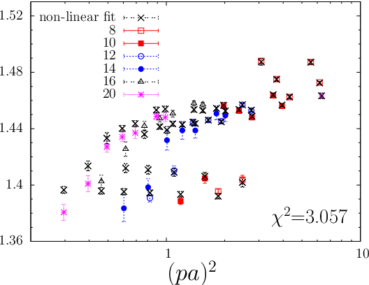
In Figure 8 (left) we show the error as functions of and for the one-loop case. As discussed in the example of Section 5.2 the plot contains data for lattice sizes . One recognizes several plateaus for the fit error . They prevent the determination of one optimal together with its attached fit parameters. But rather they suggest to average over the smallest possible . In Figure 8 (right) we show the values of the constant for the smallest which agree within errors.
Averaging over these data we obtain . We notice that this value is stable with respect to the introduction of weights proportional to the inverse of . The same holds for two and three loops.
Another requirement for an efficient fit is a suitable relation of number of data points to the number of fit parameters. In Table 3 this can be read off for all considered orders.
| one-loop | |||
| 1.244 | 13 | 43 | 0.52562(85) |
| 1.306 | 12 | 37 | 0.52582(148) |
| 1.315 | 11 | 31 | 0.52463(77) |
| 1.362 | 14 | 49 | 0.52466(64) |
| 1.381 | 15 | 55 | 0.52565(90) |
| 1.430 | 14 | 49 | 0.52615(150) |
| 1.449 | 13 | 43 | 0.52469(80) |
| 1.464 | 16 | 61 | 0.52463(66) |
| average : | 0.52523(95) | ||
| two-loop | |||
| 2.769 | 11 | 31 | 1.4883(52) |
| 2.901 | 10 | 25 | 1.4910(87) |
| 2.941 | 14 | 49 | 1.4865(51) |
| 3.057 | 13 | 43 | 1.4864(74) |
| 3.064 | 16 | 61 | 1.4852(38) |
| 3.105 | 13 | 43 | 1.4860(40) |
| 3.123 | 12 | 37 | 1.4878(13) |
| 3.146 | 15 | 55 | 1.4855(66) |
| average: | 1.4872(57) | ||
| three-loop | |||
| 3.869 | 12 | 25 | 5.04(19) |
| 4.117 | 11 | 21 | 4.66(35) |
| 4.455 | 11 | 21 | 5.02(23) |
| 4.485 | 13 | 29 | 5.14(18) |
| 4.753 | 12 | 25 | 4.83(31) |
| 4.913 | 16 | 41 | 5.23(17) |
| 5.084 | 10 | 17 | 4.62(48) |
| 5.104 | 15 | 37 | 5.03(28) |
| average: | 4.94(27) |
 |
 |
The value almost perfectly coincides with the exactly known constant given in (55) and the estimated error is small. This is a clear indication that we have reached a sufficient good accuracy of the accumulated data in the NSPT approach and the proposed fitting procedure for handling both and effects works well. For two-loop order the corresponding results are shown in Figure 9. Averaging over the eight best values we get .
Three-loop data are available for lattice sizes only. Therefore, the fits have to be performed with a smaller set of input numbers. From Table 3 one can deduce that the three-loop fit has the least accuracy. The results are shown in Figure 10.
 |
 |
The average yields which is supported by the Figure.
A major source of indetermination in our three loop analysis comes from the extrapolation . For three sizes () we only have four values of . The number given above is obtained from a quadratic fit used for one- and two-loop cases as well. Computing from a linear -fit and using otherwise the same strategy we obtain which differs about from the quadratic extrapolation. On the contrary, the one- and two-loop constants are practically not affected by the two extrapolations. For the linear extrapolation we get and .
6.2 A first comparison to MC data
Using the definition (6) as in NSPT in the gluon propagator and the Faddeev-Popov operator (24) for the calculation of the ghost propagator, the Berlin Humboldt University group has obtained Monte Carlo results for the two propagators in Landau gauge and the resulting running gauge coupling [38]. Maximizing the “linear” gauge fixing functional as a preconditioner, the final gauge fixing was organized to minimize
| (68) |
with an iterative scheme following (11), actually in a parallelized multigrid realization of Fourier acceleration (16).
Since it is assumed that non-perturbative contributions dominate mainly the intermediate and infrared momentum range, it is of interest here to compare directly the perturbative ghost dressing function obtained in NSPT with its Monte Carlo counterpart for each common momentum 4-tuple.
We calculate the perturbative dressing function at a given lattice volume summed up to loop order for a given lattice coupling as follows:
| (69) |
In Figure 11

we compare the perturbative ghost dressing function at lattice size with Monte Carlo data at two different values. We observe that at least three-loop accuracy is necessary to guarantee that the perturbative ghost propagator at larger () approximately describes the full two-point function in the large momentum squared region ().
7 Summary
We presented two- and three-loop results for the ghost propagator of Lattice SU(3) in Landau gauge. A careful analysis of finite volume and finite lattice size effects has been performed, whose methodology has been discussed quite in detail. The present work will be supplemented by a similar analysis for the gluon propagator (in the same gauge). This will open the way to a more careful comparison to Monte Carlo data for these quantities, which are supposed to encode informations on the confinement mechanism of non-Abelian gauge theories not only in the asymptotic infrared region, but also in the intermediate momentum range in the form of power corrections (condensates) [13] and contributions from non-perturbative excitations (vortices etc.) [14, 15] related to particular length scales.
Acknowledgements
This work is supported by DFG under contract SCHI 422/8-1, DFG SFB/TR 55 and by I.N.F.N. under the research project MI11. We acknowledge computer time made available to us by ECT∗ on the Ben system for approximately 13000 CPUh.
References
- [1] J. Greensite, Prog. Part. Nucl. Phys. 51, 1 (2003) [arXiv:hep-lat/0301023].
- [2] R. Alkofer and J. Greensite, J. Phys. G 34, S3 (2007) [arXiv:hep-ph/0610365].
- [3] J. Greensite, Eur. Phys. J. ST 140,1 (2007).
- [4] L. von Smekal, [arXiv:0812.0654[hep-th]].
- [5] C. S. Fischer, A. Maas, and J. M. Pawlowski, PoS Confinement8, 043 (2008), [arXiv:0812.2745[hep-ph]].
- [6] I. L. Bogolubsky, E.-M. Ilgenfritz, M. Müller-Preussker, and A. Sternbeck, Phys. Lett. B676, 69 (2009), [arXiv:0901.0736[hep-lat]].
- [7] C. S. Fischer, A. Maas, and J. M. Pawlowski, Annals Phys. 324, 2408 (2009), [arXiv:0810.1987[hep-th]].
- [8] V. N. Gribov, Nucl. Phys. bf B139, 1 (1978).
- [9] D. Zwanziger, Nucl. Phys. B364 127 (1991).
- [10] I. Ojima, Nucl. Phys. B143 340 (1978).
- [11] T. Kugo and I. Ojima, Prog. Theor. Phys. Suppl. 66, 1 (1979).
- [12] L. von Smekal, A. Jorkowski, D. Mehta, and A. Sternbeck, PoS Confinement8, 048 (2008), [arXiv:0812.2992[hep-th]].
- [13] Ph. Boucaud, F. De Soto, J. P. Leroy, A. Le Yaouanc, J. Micheli, O. Pene and J. Rodriguez-Quintero, Phys. Rev. D 79 014508 (2009) [arXiv:0811.2059[hep-ph]].
- [14] K. Langfeld, H. Reinhardt, and J. Gattnar, Nucl. Phys. B 621, 131 (2002) [arXiv:hep-ph/0107141].
- [15] J. Gattnar, K. Langfeld, and H. Reinhardt, Phys. Rev. Lett. 93, 061601 (2004) [arXiv:hep-lat/0403011].
- [16] For a comprehensive review see S. Capitani, Phys. Rept. 382, 113 (2003) [arXiv:hep-lat/0211036].
- [17] F. Di Renzo, E. Onofri, G. Marchesini and P. Marenzoni, Nucl. Phys. B 426, 675 (1994) [arXiv:hep-lat/9405019].
- [18] G. Parisi and Y. s. Wu, Sci. Sin. 24, 483 (1981).
- [19] G. G. Batrouni, G. R. Katz, A. S. Kronfeld, G. P. Lepage, B. Svetitsky and K. G. Wilson, Phys. Rev. D 32, 2736 (1985).
- [20] F. Di Renzo and L. Scorzato, JHEP 0410, 073 (2004) [arXiv:hep-lat/0410010].
- [21] E.-M. Ilgenfritz, H. Perlt and A. Schiller, PoS LATTICE 2007, 251 (2007) [arXiv:0710.0560[hep-lat]].
- [22] F. Di Renzo, L. Scorzato and C. Torrero, PoS LATTICE 2007, 240 (2007) [arXiv:0710.0552[hep-lat]].
- [23] F. Di Renzo, E.-M. Ilgenfritz, H. Perlt, A. Schiller and C. Torrero, PoS LATTICE 2008, 217 (2008) [arXiv:0809.4950[hep-lat]].
- [24] F. Di Renzo, E.-M. Ilgenfritz, H. Perlt, A. Schiller and C. Torrero, PoS Confinement8 050 (2009) [arXiv:0812.3307[hep-lat]].
- [25] F. Di Renzo, E.-M. Ilgenfritz, H. Perlt, A. Schiller and C. Torrero, arXiv:0910.2905[hep-lat].
- [26] D. Zwanziger, Nucl. Phys. B 192, 259 (1981).
- [27] C. Torrero, M. Laine, Y. Schroder, F. Di Renzo and V. Miccio, PoS LAT2006, 038 (2006) [arXiv:hep-lat/0609048].
- [28] C. T. H. Davies et al., Phys. Rev. D 37, 1581 (1988).
- [29] H. J. Rothe, Lattice Gauge Theories - An Introduction (2nd Edition), World Scientific, Singapore (1997).
- [30] C. Torrero, PhD thesis, Parma University (2006).
- [31] J. A. Gracey, Nucl. Phys. B 662 (2003) 247 [arXiv:hep-ph/0304113].
- [32] H. Kawai, R. Nakayama and K. Seo, Nucl. Phys. B 189 40 (1981).
- [33] A. Hasenfratz and P. Hasenfratz, Phys. Lett. B 93 165 (1980).
- [34] M. Lüscher and P. Weisz, Nucl. Phys. B 452 234 (1995) [arXiv:hep-lat/9505011].
- [35] C. Christou, A. Feo, H. Panagopoulos and E. Vicari, Nucl. Phys. B 525, 387 (1998) [Erratum-ibid. B 608, 479 (2001)] [arXiv:hep-lat/9801007].
- [36] F. Di Renzo, V. Miccio, L. Scorzato and C. Torrero, Eur. Phys. J. C 51, 645 (2007) [arXiv:hep-lat/0611013].
- [37] M. Constantinou, V. Lubicz, H. Panagopoulos and F. Stylianou, JHEP 0910 064 (2009) arXiv:0907.0381[hep-lat].
- [38] C. Menz, diploma thesis, Humboldt-Universität zu Berlin (2009); we acknowledge receiving those data prior to publication.