On Channel-Discontinuity-Constraint Routing in Wireless Networks
Abstract
Multi-channel wireless networks are increasingly being employed as infrastructure networks, e.g. in metro areas. Nodes in these networks frequently employ directional antennas to improve spatial throughput. In such networks, given a source and destination, it is of interest to compute an optimal path and channel assignment on every link in the path such that the path bandwidth is the same as that of the link bandwidth and such a path satisfies the constraint that no two consecutive links on the path are assigned the same channel, referred to as “Channel Discontinuity Constraint” (CDC). CDC-paths are also quite useful for TDMA system, where preferably every consecutive links along a path are assigned different time slots.
This paper contains several contributions. We first present an distributed algorithm for discovering the shortest CDC-path between given source and destination. For use in wireless networks, we explain how spatial properties can be used for dramatically expedite the algorithm. This improves the running time of the centralized algorithm of Ahuja et al. for finding the minimum-weight CDC-path. Our second result is a generalized -spanner for CDC-path; For any we show how to construct a sub-network containing only edges, such that that length of shortest CDC-paths between arbitrary sources and destinations increases by only a factor of at most . We propose a novel algorithm to compute the spanner in a distributed manner using only messages. This scheme can be implemented in a distributed manner using the ideas of [4] with a message complexity of and it is highly dynamic, so addition/deletion of nodes are easily handled in a distributed manner. An important conclusion of this scheme is in the case of directional antennas are used. In this case, it is enough to consider only the two closest nodes in each cone.
1 Introduction
Wireless infrastructure networks (WINs) are gaining prominence as they are being increasingly deployed in metro areas to provide ubiquitous information access [2]. WINs provide a low-cost scalable network, support broadband data, and allow use of unlicensed spectrum. WINs have a wide area of applications, including public internet access [2], PORTAL [8], video streaming [19], and underground mining [15]. In order to increase the bandwidth in the WINs, nodes employ multiple wireless transceivers (interface cards) to achieve simultaneous transmission/reception over multiple orthogonal channels.
Recent research has focused on effectively harvesting the available bandwidth in a wireless network. The wireless interference constraint is the key factor that limits the achievable throughput. The interference is encountered in two ways: (1) a node may not receive from two different nodes on the same channel at any given time; and (2) a node may not receive and transmit on the same channel at any given time. Moreover, if omnidirectional antenna is employed, then there may be at most only one node transmitting on a channel in the vicinity of a node that is receiving on that channel. The interference constraints in wireless networks may be divided into two categories [1]: inter-flow and intra-flow. The inter-flow interference refers to the scenario where two links belonging to different flows cannot be active (on the same channel) at the same time as one receiver will experience interference due to the other transmission. The intra-flow interference refers to the scenario where two links belonging to the same flow cannot be active (on the same channel) at the same time. The same problem arises also in the TDMA setting, where a node can be used for streaming applications, but has to receive and transmit messages in different time slots.
Prior Work: The problem of routing and channel assignment in WINs refers to computing paths and channel assignment on the paths such that there are no inter-flow and intra-flow interferences. If the bandwidth of a link is , then the end-to-end throughput on the path is also as all the links in the path can be active simultaneously. The problem of joint routing and channel assignment is hard when nodes employ omnidirectional antennas, hence is typically solved as two independent sub-problems. For a given set of calls where routing is known, the problem of channel assignment may be mapped to distance-2 vertex and edge coloring problems [7]. Using such a mapping, the objective is to compute channel assignment satisfying the limit on the number of transceivers at each node. Distance-2 vertex and edge coloring problems are well known NP-hard problems, hence the problem of channel assignment for networks employing omnidirectional antennas. Various approximation algorithms and heuristics have been developed for distance-2 coloring with different objectives, such as minimizing interference, maximizing throughput, and minimizing the number of required channels [30, 21, 17, 6, 34, 13, 5] . An approach based on balanced incomplete block design is developed in [14] to assign channels for each interface card such that the communication network is 2-edge-connected with minimum interference. In [27], a heuristic based on random channel assignment policy is developed to maintain connectivity of the network.
Among the works that compute paths for multi-channel networks, [10] develops a routing protocol to find an efficient path with low intra-flow interference, by taking into account link loss rate, link data rate, and channel diversity. In [29], shortest path with low interference is computed based on an extension to the AODV protocol to account for (inter- and intra-flow) interference and link data and loss rates. In the space of wireless network design for a given static traffic, centralized and distributed approaches for joint channel assignment and routing in the multi-interface WMN with the objective of maximizing throughput are developed in [24, 23, 3, 20], while [16] considers the objective of achieving a given data rate.
It has been shown in [36, 37, 28] that the capacity of WINs may be further improved by increasing spatial reuse by employing directional antennas. The problem of channel assignment in networks employing directional antennas may be mapped to the edge-coloring problem [22]. In [9], a network architecture with nodes employing non-steerable directional antennas is developed. The authors develop approaches for routing and channel assignment by considering tree-based topologies rooted at “gateway” nodes.
There are indications that the problem of finding a path and channel assignment such that all links can be active simultaneously is NP-complete when nodes employ omnidirectional antennas. Our algorithms are designed for the frequent cases for which the effect of interference can be ignored. For example, when directional antennas are used, as their prices and accuracy are rapidly improving, the nodes may be carefully placed such that any two independent links can use the same channel.
The first work addressing joint routing and channel assignment in WINs under such scenarios is the recent paper by Ahuja et. al. [1]. In this case, the path bandwidth will be the same as an individual link bandwidth if no two consecutive links on the path are assigned the same channel. We refer to the constraint on channel assignment as channel discontinuity constraint (CDC) and any path that satisfies the constraint as a CDC-path. In graph theory literature, CDC-paths are referred to as “properly edge-colored” paths, where channels correspond to colors. From now on, whenever it is mentioned that a CDC-path is found, it is not mentioned explicitly but it is implied that a channel assignment is also found.
We can overcome, to some extent, the difficulties that interference causes in the case of omnidirectional antennas using the known technique of network coding. Consider a streaming application, where node forwards the message to node , and receives the message at the same time from . Meanwhile, node forwards a message received earlier from to . In the case where omnidirectional antennas are used, and we have applied the CDC-path protocol, it is quite possible that the frequency of transmission of both and is , as it is different than the frequency used by (see Figure 1). However, as demonstrated in the paper by [38], since “knows” it can subtract it from the combined signal . See [38] for details. However, this is not a trivial hardware modification, so we would concentrate in this paper mostly with other applications where CDC path are useful.
Motivation: As stated, CDC-paths are particularly useful in streaming applications where the transmissions are continuous and any period of inactivity reduces bandwidth. CDC-paths are also quite useful in the context of a TDM or FDM/TDM system, where the channel may be thought of as a time slot or a combination of frequency and time slot. In TDM systems, it is desirable to assign different time slots to adjacent transmissions along the path and this corresponds exactly to the Channel Discontinuity Constraint where each channel is a time slot. Thus, if and are adjacent links along the path, the throughput is maximized when they are using different time slots. Now, because of other “conversations” which have ended, certain time slots may become available and finding new CDC-paths may help maintain the maximum bandwidth.
Our Contributions: We present a distributed algorithm for finding the shortest CDC-path between two nodes in a graph. The algorithm requires the exchange of fixed-size messages in total ( per node) where is the number of nodes. This improves the previous algorithm presented in [1] which is centralized, and requires running time.
The second contribution is the construction of a sparse graph which is a -Spanner for the problem of CDC routing, where is a controlled parameter. The number of links in is . By spanner, we mean that for any fixed as close as one wishes to , and for any pair of nodes and in the network , if contains a route between then so does the spanner , and its length is longer than the original route by only a factor of . Our spanner is based on the Yao graph[35]. The basic idea is that at a node, we divide the region around the node into sectors and store only a few neighbors in each sector. The parameter is dependent on the number of sectors. This is particularly applicable when using directional antennas. For example, if the antennas’ covering range can be abstracted as a sector of angle degrees, then by storing for every node just the few neighbors in each sector, we retain connectivity and gain routes which are no longer than times the theoretical bounds. This spanner is also highly dynamic, so insertion/deletion of links is carried out easily.
The rest of the paper is organized as follows. In Section 2, we discuss the network model and interference constraints. In Section 3, we review the technique developed in [1] that explains how the CDC problem can be expressed as a matching problem. In Section 4, we present a distributed algorithm for finding a single CDC-path between and which requires the sending of a total of messages. In Section 5, we discuss a t-spanner for WINs containing links. Finally, we present the conclusion and some future work.
2 System Model
Consider a multi-channel wireless network, where denotes the set of orthogonal channels each with bandwidth . Let . Let denote the set of nodes each equipped with transceivers that may be tuned to any of the orthogonal channels. Let be the transmission range of a node. We refer to two nodes as neighbors if the Euclidean distance between them is not greater than . Let denote the connectivity graph, where denotes the set of links. A link connects two neighboring nodes.
WINs may be designed such that the number of links that can be active simultaneously can be maximized. A node is said to be collinear with a transmission from to if node cannot receive on the same channel as that used by the transmission from to . The interference at node due to the transmission from to results in signal-to-noise ratio that is lower than the threshold for decoding the received signal. The collinearity constraint results in the dependence on channel assignment between links that are not adjacent to each other. (hence resulting in distance-2 coloring problems).
While the collinearity constraint is inherent in networks employing omnidirectional antennas, they can be eliminated completely by careful placement of nodes when directional antennas are employed. In such carefully planned wireless infrastructure networks, there are only two interference constraints: (1) a node may not receive on a channel from more than one node at the same time; and (2) a node may not transmit and receive on a channel at the same time. These two constraints may lead to intra-flow interference, however it is limited to only two adjacent links. In order to avoid intra-flow interference, no two consecutive links in the path are assigned the same channel.
We assume that the list of channels that a node can transmit/receive on is known at all times. The channels available on a link between neighboring nodes and is simply the set of common channels at the two nodes. Every call is assumed to have a bandwidth requirement of one channel capacity. We assume that calls are bidirectional and the same channel will be shared in both directions on a link. We also do not care if the communications required for the algorithm satisfy CDC, since, typically, a control channel is used to transmit network-related information rather than the actual data transmissions in the network and the control messages are also typically very short.
3 Problem Formulation
Problem Statement: Given a multi-channel wireless network with no collinear interference, the set of available channels on every link, the cost of the links, and a node pair , find the shortest path between and along with a channel assignment on every link of the path such that no two consecutive links in the path are assigned the same channel.
Definition 1.
We call a path a CDC-path if we can assign channels to each link along this path and no two adjacent links have the same channel assigned.
Ahuja et. al. [1] showed the equivalence of computing the minimum cost CDC-path to the computation of minimum cost perfect matching (MCPM) using Edmonds-Szeider (ES) expansion for nodes. For the sake of completeness, we give a description of their method here. In the ES-expansion graph, we expand each node , except the source and destination nodes, into sub-nodes, denoted , each pair corresponding to a channel . We also add sub-nodes . Each pair is connected to each other and we refer to these links as channel link. Every sub-node is also connected to and . Assign cost 0 to all the above links in the expanded node. Ahuja et. al. [1] also noted that these expansions may be modified to reduce the number of links in the following manner. For links with two or less channels available on them, expand as before. For links with three or more channels, the additional links may be eliminated since, for any CDC-path which uses this link, we can always find a channel assignment from the three corresponding channels.
If two nodes and are connected in and have a set of channels available between them, then the sub-nodes and corresponding to the available channels are also connected. Connect and to the sub-nodes of its neighboring nodes corresponding to the available channels between them.
Now, the problem of computing the shortest CDC-path is the same as computing the minimum-cost perfect matching in the expanded graph. A perfect matching in a graph is a set of non-adjacent edges, i.e., no two edges share the same vertex, such that all the vertices in the graph are covered. A minimum cost perfect matching is defined as a perfect matching where the sum of the cost of the edges in the matching is minimum.
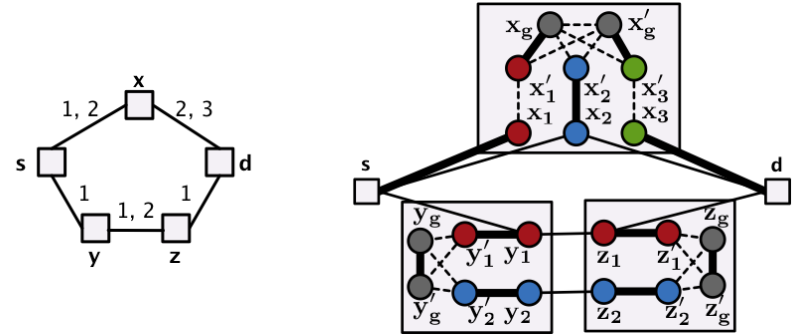
We illustrate the equivalence of MCPM and CDC-path using an example. Consider the example network and its ES-expansion as shown in Figure 2. Numbers over links represent the available channels on the corresponding links. The link costs are assumed to be 1 for this illustration, hence the objective is to compute the minimum hop CDC-path. The edges in the matching are shown in bold in the expanded graph. The nodes not present in the shortest path from to would find matching within itself (see nodes and ). Intermediate nodes (if any) in the shortest to path will have exactly two incident external edges in the matching (see node ). Clearly, the returned path –– with channels 1 and 3 over links – and –, respectively, is the shortest CDC-path between and in terms of hop length.
The best known sequential implementation of Edmonds’ minimum cost perfect matching algorithm is by Gabow [11] with complexity where and are the number of nodes and links respectively. Since the number of nodes in the expanded graph is and the number of links is , the complexity of computing a solution to MCPM is . However, this complexity can be reduced by observing that most of the matching computed in the MCPM are within the nodes itself (except for the links involved in the path). A closer look reveals that we can start with an expanded graph with a partial matching where all the internal edges and at node and and are matched. If this is the case, then the problem of computing the minimum cost perfect matching is transformed to computing the minimum cost alternating path. We thank Kasturi Varadarajan for this observation. It is interesting to note that Varadarajan and Agarwal have designed algorithms[31, 32] for exactly[31] and approximately[32] finding a minimum-weight matching in a geometric setting. In the following sections, we develop a distributed algorithm to compute the shortest alternating path with better bounds than Ahuja et. al.[1].
4 Finding the Shortest CDC Path
We are given the expanded graph together with the matching of zero weight (all vertices except and internally matched). For any node , let denote the mate of in the matching .
Definition 2.
Between any two nodes and , we define an alternating path to be a path with alternating unmatched and matched edges.
Definition 3.
For any node , we define a co-link path from to as an alternating path where .
Our algorithm shares many ideas with Edmonds’ algorithm. It works by finding minimum weight co-link paths similar to each phase of Edmonds’ algorithm. Each node maintains two distances: and , corresponding to the minimum weight co-link paths to itself and respectively. Through the course of the algorithm, each node is given labels from the set . We say a node if it is given an label and similarly for the other labels. Initially, and every other node . Each node also maintains the current known distances and of its neighbors in . During the algorithm, certain odd subsets of vertices are termed as blossoms.
Definition 4.
A blossom is an odd circuit in for which is a perfect matching for all vertices in except one. The lone unmatched vertex is termed as the base of the blossom.
Through the course of the algorithm, a node may be added to one or more blossoms. Hence, it maintains the ID of the base of the outermost blossom it belongs to (the reader is referred to the book by Lawler[18] for the definition of outermost blossom). Let denote this ID. When a node is added to for the first time, it stores the corresponding ID of the parent of , . When a node is added to for the first time, if it is not the base of a blossom, it stores the corresponding ID of the parent of , . If it is the base of a blossom , is now a subblossom of a new blossom . In this case, stores the edge which is the first unmatched edge in connected to and not in . For more details, see [18].
The algorithm works in three phases: FINDMIN, BLOSSOM and GROW. Before we proceed, let us define a few expressions. For a node , let
Each node maintains an “examined” state for each neighbor . Let and . The steps of FINDMIN are as follows.
(Step ) Each node computes and the corresponding .
(Step ) If , it sends a message to requesting . If , the two nodes belong to the same blossom and no blossom discovery is necessary. In this case, marks as examined. The process repeats from Step to discover a new . This continues until the minimum is achieved for a node or a node and .
(Step ) Each node sends a message to in the following manner. Each node waits until it has received messages from all its children . Then, finds the minimimum where . sends the message to its parent where is the edge for which the minimum was attained. For nodes in blossoms, the parent depends on which set it was added to first. When receives all messages, it sends a message to nodes and where edge is the one for which the minimum was attained. and mark each other as examined.
The second stage of the algorithm is the BLOSSOM phase which executes the blossom discovery process for an edge corresponding to a new outermost blossom . This is done by sending messages from and towards till the base of the blossom is found. The way in which these messages are sent follows the description given by Shieber and Moran[26]. Once this is done, sends messages throughout the blossom and informs all nodes of their membership by assigning . In addition, for all new nodes in the blossom, the corresponding parents and the corresponding alternate distance or are assigned.
The GROW phase extends the tree by adding one node to and one to . Let be the edge used to add to and to . is added to and to . The labels are removed and the following values are assigned:
sends a message to all its neighbors informing them of its new label and its distance .
The algorithm works in iterations. In each one, it executes FINDMIN. Let . If , we execute BLOSSOM. Otherwise, we execute GROW. The overall steps of the algorithm are outlined in Figure 3.
Algorithm SHORTEST-CDC Set and , Set and for all Execute FINDMIN. Let be the edge for which the minimum was attained. if then Execute BLOSSOM else Execute GROW Once is removed from F, the algorithm terminates.
We now prove the correctness of the algorithm by showing that, at each stage of SHORTEST-CDC, the same edge is selected as in each phase of Edmonds’ algorithm. From now on, whenever we mention Edmonds’ algorithm, we refer to each phase of Edmonds’ algorithm.
Fact 1.
For each edge ,
We now give an outline of Edmonds’ algorithm for the sake of completeness. For more details, see [18]. Each node is associated with a dual variable and each odd subset of vertices is assigned a dual variable . Note that only for blossoms and for every other odd subset. Each node and blossom belong to one of three sets . Initially, and everything else is in . An edge is termed as tight if . At each step, Edmonds’ algorithm searches for tight edges in order to close blossom or grow the tree. If there are no tight edges, it makes a dual change. We choose , where
| (1) | |||||
| (2) | |||||
| (3) |
For each node , we set and for each node , . For each outermost blossom (resp. ), (resp. ). Now, the only case where a blossom is when it shrunk at the start of the algorithm. In our case, there are no shrunk blossoms at the beginning. Hence, we only need to worry about and .
Lemma 1.
For each edge ,
throughout the course of Edmonds’ algorithm.
Proof.
Since each edge is tight throughout the course of the algorithm,
| (4) |
This, combined with Fact 1 gives the desired result. ∎
Note that is the weight of the shortest co-link path to . This leads to the following lemma whose proof is in the appendix.
Lemma 2.
For each node ,
Using the above lemma, we can prove that our algorithm works in a similar manner to Edmonds’ algorithm.
Lemma 3.
If edge becomes tight at some point in Edmonds’ algorithm, it becomes tight at the same point in the algorithm SHORTEST-CDC.
Proof.
At some intermediate step of Edmonds’ algorithm, let some value be chosen as the dual change for that step. Let be the dual variables of any node before the dual change of . Let . Now, according to Lemma 2,
| (5) |
The value of is given by where and are given by Equations 2 and 3. This is because, at the start of the algorithm, there are no blossoms. Hence, no non-trivial -blossoms are found and Equation 1 never occurs. We may compute .
Taking the case of , we have,
| (6) | |||||
| (7) | |||||
| (8) |
The above equations follow from Equation 5 and Lemma 1. In the case of , we may similarly compute it as
| (9) | |||||
| (10) | |||||
| (11) | |||||
| (12) |
Since , Equations 8 and 12 are exactly the values computed by the algorithm SHORTEST-CDC during the FINDMIN phase. Hence, the lemma is proved. ∎
Theorem 1.
The algorithm SHORTEST-CDC finds the shortest CDC path from to using fixed-size messages.
Proof.
From Lemma 3, it is clear that the steps of Algorithm SHORTEST-CDC follow the steps of Edmonds’ algorithm exactly. Hence, we indeed find the shortest augmenting path from to . This implies that we have found the shortest CDC path from to .
We now analyze the communication complexity of Algorithm SHORTEST-CDC. There are three main phases to the algorithm: (i) The FINDMIN phase. Here each node scans its adjacent edges at most once through the algorithm. Hence, each edge is scanned at most twice leading to a message complexity of . (ii) The GROW phase. Clearly, at each GROW phase, messages are sent leading to a total message complexity of . (iii) The BLOSSOM phase. Using the approach of [26], for each edge, we can achieve the backward and forward processes using messages. There can be no more than blossoms found during the course of the algorithm leading to a complexity of . Note that, although the approach of [26] is for unweighted graphs, since we do not have blossom expansions, their method can be used exactly since the rest of the blossom discovery is identical to unweighted graphs [18]. Each message sent is of fixed size. Hence, the total number of fixed-size messages sent during the algorithm is . ∎
It is worth noting that if the graph is unweighted or if the edge weights are integers, then we have several advantages. The complexity of FINDMIN is reduced since there is no need to send messages back to . The blossom discovery process becomes simpler by discovering all blossom edges at the same time. We can find a path using messages where is the length of the shortest CDC path.
5 Spanner for CDC Routing
In this section, we discuss a spanner for Channel-Discontinuity-Constraint routing in wireless networks. We are given a graph where is the set of nodes in and is the set of links between nodes, and the set of channels available at each node . Let denote the euclidean distance between and . The weight of every link is given to be . The cost of a path is the sum of the weights of the links along and is denoted by .
Definition 5.
Let denote the cost of the shortest CDC-path from to in . If there is no such path, then the cost is infinity. We say that a graph where is a CDC -Spanner of if and only if for every , where is a constant.
Definition 6.
Let denote a partition of nodes in into maximally disjoint sets such that for every . We define the type of a node , denoted by , to be the set containing . If is the number of channels available in the network, then, .
The above definition of CDC spanners is based on the definition of spanners for Unit Disk Graphs in [33] but is equally relevant in the case of networks using directional antennas. The CDC t-Spanner , which is based on the Yao graph [35], is created as follows. The set of links in is obtained in the following manner. For each node , divide the region around into interior-disjoint sectors centered at with opening angle . In each sector, connect to its two nearest neighbors of each type and connect these neighbors with a link. This process can be performed in a distributed manner as described later. We prove that this graph is a CDC -Spanner for the graph where . This is particularly applicable when directional antennas are used. Also, the computation of the above spanner does not require that we know in advance the specific source and destination between which a CDC path needs to be computed.
Figure 4: and are located in clusters and respectively. The only path from to is the edge which is not present in .
Remark 1.
We note that no sub-quadratic size spanner can accommodate the degenerate case where the the shortest CDC path between two nodes and is only one edge. For example, in the case where and are in two clusters and and there is only one channel shared between nodes in and nodes in (see Figure 5), all edges from to may be required. However, no routing algorithm is needed here since can check to see if is within range and transmit to it. When not considering the degenerate case, we obtain the following theorem.
Theorem 2.
is a CDC -Spanner of and where .
The following lemma was proven by Ruppert and Seidel [25] as a part of their proof of the stretch factor of the Yao Graph.
Lemma 4 (From [25]).
If there are two nodes and in a sector whose apex is and , then .
Figure 5: Nodes and are in a sector of and
.
Let be an CDC-path in where and . In the following lemmas, we assume that . The case where is discussed in Remark 1 above. We describe a procedure that shows that existence of an CDC-path in such that . Note that this is not the algorithm used it practice but is described just to show the existence of such a path. From now on, for every path we create we also assign channels to its links.
The algorithm has two major components:
Link Replacement: Each link in is replaced by a path. The resulting path , obtained by replacing all the links in , may not be simple. However, .
Untangling: A path is obtained from such that and is simple.
We divide the links in into three cases - (i) the intermediate links for , (ii) the first link and (iii) the last link .
Now, consider the first case where link is not the first or last link. We replace this link with a path in the following manner. If, for even , is a link in , the next node is . Otherwise, the next vertex of is the nearest neighbor of type either or in the sector of where is the sector containing . From , connect to the next nearest neighbor to of type the sector . Repeat for . This process is demonstrated in Figure 6. Let denote the channel assignment in to the links , and respectively. We may assign channels satisfying CDC to as follows (i) to and or to for and (ii) to .
Now, for the second case, if has exactly one channel available to it, we may only construct the above path through nodes of type . In the third case, if has exactly one channel available to it, then a path from to may not exist. However, we may construct a path from to through nodes of type .
Let be the path obtained by concatenating after (). We prove, in Lemma 5, that always exists. We also prove, in Lemma 6, that and we can assign channels to the links in satisfying CDC. However, might not be simple, since when constructing , no caution is given for not using nodes of where . This problem is resolved in Lemma 7, which shows how to create an CDC-path from , without increasing its length. The proofs of these lemmas are in the appendix.
Lemma 5.
If there is a path from to in , then the path from to in constructed by the Link Replacement Procedure exists.
Lemma 6.
for and we can assign channels to the links in satisfying the Channel Discontinuity Constraint.
Lemma 7.
If, for some , overlaps with the portion of following , then we can generate a new path such that (i) , (ii) has fewer such overlaps, and (iii) no two consecutive links are assigned the same channel.
Proof of Theorem 2.
Consider a CDC-path between nodes and . The case where the number of links in is one has been discussed in Remark 1. If the number of links in is two or more, we may obtain the path in as described in the link replacement procedure, which may not be simple. From , we may apply Lemma 7 to to remove any overlaps with followed by removal of overlaps with (for ), to obtain , a simple CDC-path in from to . Note that and cannot overlap at the same node on as the original CDC-path is simple. Since we are eliminating all overlaps of for before , this case will not occur because such a shared node will no longer be shared after the first time it is found to overlap. Hence, at each step, we reduce the number of overlaps and at the final step when we are handling , there will be no overlaps.
Our results are of a theoretical nature, since the constants in the bounds might be too large. However, we use them as evidence that, in practice, connecting every node to a small number of its nearest neighbors, in each of the sectors (lobes), either user-defined or explicitly by the directional antennas, will yield a network with almost same properties as the original network. Moreover, a close look of the proof of Theorem 2 reveals that, excluding some convoluted cases, the bounds also hold if the cost of transmitting a message between nodes is proportional to , for any .
The total number of links in seems to be since the total number of types is . We now argue that the number of links can actually be bounded by by constructing the graph in the following manner. At a node , for each pair of channels, connect to the two nearest neighbors which have these channels. Let this graph be a CDC t-spanner . The proof of the following lemma is in the appendix.
Lemma 8.
is a CDC -Spanner where and the number of links in is .
We now outline the algorithm to compute the spanner in a distributed manner using messages. Let be a node, and let be the set of sectors around . For each type , needs to know the first two nearest neighbors of type in each sector . In order to find these neighbors, sends a message, specifying the sector and type. Each node that hears the message, estimates the distance to , and picks a random backoff time during which it waits and listen to see how many nodes it hears whose distance . If when the timer of expires, it did not hear at least 2 such nodes , then broadcasts its distance . For details on the message complexity of this approach, refer to [4].
6 Simulations
We have conducted experiments to analyze the performance of SHORTEST-CDC under several settings. We consider network topologies ranging of 100 to 800 nodes distributed randomly in a region of unit2. We analyze two cases: (i) The density of the network is constant, i.e., the transmission range is inversely proportional to the number of nodes in the network and (ii) The transmission range is constant. In the first case, the transmission range varies from 11 units for 100 nodes to 4 units for 800 nodes and in the second case, the transmission range of the nodes is set at units. The number of channels available in the network is either 10 or 20. The parameters of the system under consideration are (i) The number of nodes and (ii) The number of channels available at a node. We evaluate the following performance metrics: Communication Complexity: We evaluate the dependence of the communication complexity (number of messages sent) of the algorithm on number of nodes and channels. The worst-case complexity is in the expanded graph which is a complexity of in the original network. We are interested in seeing which parameter has more effect on the communication complexity and how many messages are sent in practice.
Number of Blossoms: Since the major portion of the complexity is due to the formation and detection of blossoms in the graph, we evaluate the number of blossoms which are formed on average and correlate this with the communication complexity.
[p]
![[Uncaptioned image]](0912.4115v2/resnvsmsgs.png) Figure 7: Avg. Number of Messages vs Number of nodes in the network
Figure 7: Avg. Number of Messages vs Number of nodes in the network
![[Uncaptioned image]](0912.4115v2/resnvsbl.png) Figure 8: Avg. number of blossoms vs Number of Nodes
Figure 8: Avg. number of blossoms vs Number of Nodes
![[Uncaptioned image]](0912.4115v2/resch.png) Figure 9: Average number of Messages vs Number of Channels available at a
node
Figure 9: Average number of Messages vs Number of Channels available at a
node
Figure 9 shows the ratio of the average number of messages sent to as a function of the number of nodes in the network. Here, the total number of channels is and each node picks channels. In case of constant density, we can see that as the number of nodes increases, the ratio decreases very gradually and hence, we may infer that the dependence on the number of nodes is limited. In the case of variable density (constant transmission range), we can see that there is a steady increase in the ratio which seems to be quadratic in . This is expected since, the denser the network gets, the more the number of blossoms and our intuition is that the blossoms are the major factor in the complexity. In both cases, we can see that the number of messages does not stray far beyond and is well below . Figure 9 shows the ratio of the average number of blossoms to the number of nodes as a function of for the experiments run in Figure 9. As can be seen, it closely follows the graph of Figure 9. This leads us to conclude that the number of blossoms is the major factor in the number of messages.
Figure 9 shows the ratio of Average number of messages to as a function of the number of channels at a given node. In this case, is fixed at nodes and the number of channels is varied from to . The function appears to be close to linear. This leads us to conjecture that, the number of messages is, in practice, not quadratic in and could probably be linear.
7 Conclusion
In this paper, we studied the problem of path selection and channel assignment with channel discontinuity constraint (CDC) in a wireless infrastructure network. Given that any two independent links may share a channel, we showed that the problem of computing a CDC path is equivalent of computing the minimum weight alternating path. We developed a distributed algorithm to compute the minimum weight CDC path with fixed-size messages. Through experimental evaluations on random network topologies, we study the trends on the number of messages exchanged per path computation as the network size and number of channels increases. In addition, we develop a -spanner for CDC routing, where the number of links employed is significantly reduced yet guaranteeing that the minimum-weight CDC path in the spanner is no worse than times the minimum-weight CDC-path in the original network.
8 Acknowledgements
The work in this paper was partially supported by an NSF CAREER Grant 0348000.
References
- [1] Sandeep K. Ahuja, Abishek Gopalan, and Srinivasan Ramasubramanian. Joint routing and channel assignment in multi-channel wireless infrastructure networks. In Proceedings of BROADNETS 2008, 2008.
- [2] I. F. Akyildiz, X. Wang, and W. Wang. Wireless mesh networks: a survey. In Computer Networks, 2004.
- [3] M. Alicherry, R. Bhatia, and L. E. Li. Joint channel assignment and routing for throughput optimization in multiradio wireless mesh networks. In JSAC, 2006.
- [4] Jesus Arango, Alon Efrat, Srinivasan Ramasubramanian, Stephen Pink, and Marwan Krunz. Retransmission and backoff strategies for wireless broadcasting. Ad Hoc Networks, 8(1):77–95, 2010.
- [5] C. L. Barrett, G. Istrate, V. S. A. Kumar, M. V. Marathe, S. Thite, and S. Thulasidasan. Strong edge coloring for channel assignment in wireless radio networks. In Fourth Annual IEEE International Conference on Pervasive Computing and Communications Workshops, 2006.
- [6] A. A. Bertossi, M. C. Pinotti, and R. Rizzi. Channel assignment on strongly-simplicial graphs. In International Parallel and Distributed Processing Symposium, 2003.
- [7] H. L. Bodlaender, T. Kloks, R. B. Tan, and J. V. Leeuwen. -coloring of graphs. In The 17th Annual Symposium on Theoretical Aspects of Computer Science, 2000.
- [8] R. Bruno, M. Conti, and E. Gregori. Mesh networks: commodity multihop ad hoc networks. In IEEE Communications Magazine, 2005.
- [9] S. M. Das, H. Pucha, D. Koutsonikolas, Y. C. Hu, and D. Peroulis. Dmesh: Incorporating practical directional antennas in multichannel wireless mesh networks. In JSAC, 2006.
- [10] R. Draves, J. Padhye, and B. Zill. Routing in multi-radio, multi-hop wireless mesh networks. In International Conference on Mobile Computing and Networking, 2004.
- [11] H. N. Gabow. Data structures for weighted matching and nearest common ancestors with linking. In Proceedings of the 1st Annual ACM-SIAM Symposium on Discrete Algorithms, 1990.
- [12] Harold Neil Gabow. Implementation of algorithms for maximum matching on nonbipartite graphs. PhD thesis, Stanford University, 1974.
- [13] C.-C. Hsu, P. Liu, D.-W. Wang, and J.-J. Wu. Generalized edge coloring for channel assignment in wireless networks. In International Conference on Parallel Processing, 2006.
- [14] H.-J. Huang, X.-L. Cao, X.-H. Jia, and X.-L. Wang. A bibd-based channal assignment algorithm for multi-radio wireless mesh networks. In International Conference on Machine Learning and Cybernetics, 2006.
- [15] G. A. Kennedy and P. J. Foster. High resilience networks and microwave propagation in underground mines. In The 9th European Conference on Wireless Technology, 2006.
- [16] M. Kodialam and T. Nandagopal. Characterizing achievable rates in multi-hop wireless networks: the joint routing and scheduling problem. In Proceedings of the ACM Mobicom, 2003.
- [17] S. O. Krumke, M. V. Marathe, and S. S. Ravi. Models and approximation algorithms for channel assignment in radio networks. In Wireless Networks, 2001.
- [18] E Lawler. Combinatorial Optimization: Networks and Matroids. Holt, Rinehart, Winston, 1976.
- [19] N. Mastronarde, Y. Andreopoulos, M. V. D. Schaar, D. Krishnaswamy, and J. Vicente. Cross-layer video streaming over 802.11e-enabled wireless mesh networks. In ICASSP, 2006.
- [20] X. Meng, K. Tan, and Q. Zhang. Joint routing and channel assignment in multi-radio wireless mesh networks. In ICC, 2006.
- [21] K. N. Ramachandran, E. M. Belding, K. C. Almeroth, and M. M. Buddhikot. Interference-aware channel assignment in multi-radio wireless mesh networks. In INFOCOM, 2006.
- [22] R. Ramanathan, J. Redi, C. Santivanez, D. Wiggins, and S. Polit. Ad hoc networking with directional antennas: A complete system solution. JSAC, 23:496–506, 2005.
- [23] A. Raniwala and T.-C. Chiueh. Architecture and algorithms for an ieee 802.11-based multi-channel wireless mesh network. In INFOCOM, 2005.
- [24] A. Raniwala, K. Gopalan, and T.-C. Chiueh. Centralized channel assignment and routing algorithms for multi-channel wireless mesh networks. In ACM SIGMOBILE Mobile Computing and Communications Review, 2004.
- [25] J. Ruppert and R. Seidel. Approximating the -dimensional complete Euclidean graph. In Proc. 3rd Canad. Conf. Comput. Geom., 1991.
- [26] Baruch Shieber and Shlomo Moran. Slowing sequential algorithms for obtaining fast distributed and parallel algorithms: maximum matchings. In PODC ’86: Proceedings of the fifth annual ACM symposium on Principles of distributed computing, pages 282–292, New York, NY, USA, 1986. ACM.
- [27] M. Shin, S. Lee, and Y.-A. Kim. Distributed channel assignment for multi-radio wireless networks. In MASS, 2006.
- [28] A. Spyropoulos and C. S. Raghavendra. Capacity bounds for ad-hoc networks using directional antennas. In IEEE International Conference on Communications, 2003.
- [29] A. P. Subramanian, M. M. Buddhikot, and S. Miller. Interference aware routing in multi-radio wireless mesh networks. In 2nd IEEE Workshop on Wireless Mesh Networks, 2006.
- [30] A. P. Subramanian, H. Gupta, and S. R. Das. Minimum interference channel assignment in multi-radio wireless mesh networks. In SECON, 2007.
- [31] Kasturi R. Varadarajan. A divide-and-conquer algorithm for min-cost perfect matching in the plane. In Proceedings of FOCS ’98, 1998.
- [32] Kasturi R. Varadarajan and Pankaj K. Agarwal. Approximation algorithms for bipartite and non-bipartite matching in the plane. In Proceedings of SODA ’99, 1999.
- [33] Yu Wang and Xiang-Yang Li. Distributed spanner with bounded degree for wireless ad hoc networks. In IPDPS ’02: Proceedings of the 16th International Parallel and Distributed Processing Symposium, 2002.
- [34] L. Xu, Y. Xiang, and M. Shi. A novel channel assignment algorithm based on topology simplification in multi-radio wirelesss mesh networks. In 25th IEEE International Performance, Computing, and Communications Conference, 2006.
- [35] Andrew C Yao. On constructing minimum spanning trees in k-dimensional spaces and related problems. Technical report, Stanford University, 1977.
- [36] S. Yi, Y. Pei, and S. Kalyanaraman. On the capacity improvement of ad hoc wireless networks using directional antennas. In ACM international symposium on Mobile ad hoc networking and computing, 2003.
- [37] J. Zhang and S. C. Liew. Capacity improvement of wireless ad hoc networks with directional antennae. In IEEE Vehicular Technology Conference, 2006.
- [38] Shengli Zhang, Soung Chang Liew, and Patrick P. Lam. Hot topic: physical-layer network coding. In MobiCom ’06: Proceedings of the 12th annual international conference on Mobile computing and networking, 2006.
Appendix A Proof of Lemma 2
Lemma 2. For each node ,
Proof.
The proof of this lemma follows from the description given by Gabow [12]. Let the shortest alternating path from tox ending in an unmatched edge be . The weight of this path is given by,
| (13) | |||||
by Fact 1, since the weights of the matched edges is zero.
Since each edge is tight, we have . Substituting this into Equation , we get the result of the lemma, i.e.,
| (16) |
since is not part of any blossoms(it can only be the base of some blossom). ∎
Appendix B Proof of Lemmas from Section 5
Lemma 5. If there is a path from to in , then the path from to in constructed by the Link Replacement Procedure exists.
Proof.
Consider a link . We first look at the case where is an intermediate link. Consider a step of the Link Replacement procedure where we are at a node , for some even . Now, in the sector of containing , we check if the is among the two nearest neighbors of type . If this is the case, we may directly connect to it. Now, since is a neighbor of and for each , , we have the fact that is a neighbor of . Hence, there cannot be a case that does not have any neighbors of type . So, we will always be able to reach and hence, there is a path from to in .
In the case where is the first link, we may be restricted to paths through nodes of type and the above reasoning holds good in this case also. In the case where is the last link and when has only one channel, say , we may not find a path from to . If we try to find a path from to through nodes of type , then we may get stuck if has no neighbors of type . On the other hand, if we find a path through nodes of type , we can only assign channel to links along this path and hence, it will not satisfy CDC. However, we know that has more than one channel since we are assuming that and hence, there are two or more edges in . Therefore, we may find a path from to through nodes of type .
∎
Lemma 6. for and we can assign channels to the links in satisfying the Channel Discontinuity Constraint.
Proof.
Let be the portion of from to for some . Consider the path from to consisting of nodes , where is even, in together with the node . Note that is not necessarily a CDC-path. The links along with the link as shown in Figure 6 constitute the links in . For each node on this path, from Lemma 4, we know that
| (17) |
See Figure 6. Now, by summation over all even , we get
Rearranging (details omitted), we get
| (19) |
where . Now, we have in , for each , where is even and , from Lemma 4,
| (20) |
since . Combining equations 19 and 20, we get . Hence,
| (21) |
Hence, for . Consider that the nodes and share the channel and that the links and are assigned the channels and respectively. We now have a channel assignment for the path because for every set of nodes for along this path when is even, we can assign channels or depending on whether and are of type or . Finally, we assign the channel to the link . This channel assignment is shown in Figure 6. Hence, repeating this over all links in , we have a channel assignment for links in and , for . ∎
(marked as a BLUE dashed path) removes the portion of from back to itself.
(marked as a BLUE dashed path) consists of the portion of from to , the links and followed by the portion of from to .
Lemma 7. If, for some , overlaps with the portion of following , then we can generate a new path such that (i) , (ii) has fewer such overlaps, and (iii) no two consecutive links are assigned the same channel.
Proof.
Let the portion of preceding be and that following be . Now, either or or both share nodes with . We can obtain a new CDC-path as follows.
We show the CDC-path for the case where shares nodes with . Assume that uses a node in and this is the last node in which is in . Let the channel assigned to the outgoing link from to a node in the path be as shown in Figure 10. There are three cases for - (i) and , (ii) and (iii) . Now, we obtain a new path (not necessarily simple) satisfying CDC by replacing the portion of from to with a new path which we describe below.
There are two cases for the node depending on whether is odd or even. We first handle the case when is odd. In this case, and are in the cone of which contains . This is because, according to the link replacement procedure, from , we would have picked the two nearest neighbors in the cone of containing . If is odd, the two cases where and are depicted in Figure 10.
If , we obtain by going from to along . The path obtained using this satisfies CDC because, according to the channel assignments for , the link is not assigned channel and the link is assigned channel which is different from . We are not increasing the cost of by doing this. This is depicted in Figure 10a.
If , we obtain by going from to along and adding the links and . Assigning channels and to links and respectively, we get a path from to . This is depicted in Figure 10b. Now, we prove that the cost of is no larger than the cost of . Let the portion of from to be and the portion from to be . Applying triangle inequality in the triangles and , we have and . Adding, we get,
Adding the cost of the portions of from to and from to , we get,
| (23) | |||||
Since cost of the portions of from to and from to are not less than and respectively, . The case where overlaps with is analogous to the above case. Instead of using the last node of overlap, we would use the first node of overlap to obtain the shortened path from to . The number of overlaps in is less than that in because in , the portion of the path from to now no longer overlaps with the portion from to . ∎
Lemma 8. is a CDC -Spanner where and the number of links in is .
Proof.
Consider an edge which is part of some CDC-path in . Note that we are still under the assumption that the number of nodes in is greater than 2. Let us consider the three cases: (i) is one of the intermediate links other than the first and last link, (ii) is the first link in and (iii) is the last link in . Consider the first case. If the only channel shared between and is , then has at least one more channel, say , available at it. Now, we may construct a path through nodes which have channels . This will satisfy CDC because we may assign channels and alternately to edges in this path. If the number of channels shared is two or more, then, by our construction, we may still construct a path as before between and through nodes which have any pair of channels from the shared channels. In the remaining cases for , we may still construct paths from to because, again, at least one of them has two or more channels. Lemmas 5, 6 and 7 still hold for these paths. Hence, is a CDC -Spanner for . The number of links in at a node is per sector since we have three links for each pair of channels and the total number of pairs is . Hence, the total number of links in is .
∎