Structure-Preserving Discretization of Incompressible Fluids

Let $M\subset\mathbb{R}^{n}$ be an arbitrary compact manifold, possibly with boundary (where $n$ denotes the dimension of the domain, typically, 2 or 3), and ${\rm SDiff}(M)$ be the group of smooth volume-preserving diffeomorphisms on $M$. As was shown in [2], the motion of an ideal incompressible fluid in $M$ may be described by a geodesic curve $g_{t}$ in ${\rm SDiff}(M)$. That is, ${\rm SDiff}(M)$ serves as the configuration space—a particle located at a point $x_{0}\in M$ at time $t=0$ travels to $g_{t}(x_{0})$ at time $t$. Being geodesics, the equations of motion naturally derive from Hamilton’s stationary action principle:

subject to arbitrary variations $\delta g$ vanishing at the endpoints. Here, the Lagrangian $L(g,\dot{g})$ is the kinetic energy of the fluid and $dV$ is the standard volume element on $M$. As this Lagrangian is invariant under particle relabeling—that is, the action of ${\rm SDiff}(M)$ on itself by composition on the right, the principle stated in Eq. (1) can be rewritten in reduced (Eulerian) form in terms of the Eulerian velocity $v=\dot{g}\circ g^{-1}$:

subject to constrained variations $\delta v=\dot{\xi}+[v,\xi]$ (called Lin constraints), where $\xi$ is an arbitrary divergence-free vector field—an element of the Lie algebra of the group of volume preserving diffeomorphisms—and $[\,,]$ is the Jacobi Lie bracket (or vector field commutator). There is a complex history behind this reduced variational principle which was first shown for general Lie groups by [34]; see also [2, 22, 5, 32]). As stated above, the reduced Eulerian principle is more attractive in computations because it involves a fixed Eulerian domain (mesh); however, the constrained variations necessary in this context complicates the design of a variational Eulerian algorithm.

While time integrators for fluid mechanics are often derived by approximating equations of motion, we instead follow the geometric principles described above and discretize the configuration space of incompressible fluids in order to derive the equations of motion through the principle of stationary action. Our approach uses an Eulerian, finite dimensional representation of volume-preserving diffeomorphisms that encodes the displacement of a fluid from its initial configuration using special orthogonal, signed stochastic matrices. From this particular discretization of the configuration space, which forms a finite dimensional Lie group, one can derive a right-invariant discrete equivalent to the Eulerian velocity through its Lie algebra, i.e., through antisymmetric matrices whose columns sum to zero. After imposing non-holonomic constraints on the velocity field to allow transfer only between neighboring cells during each time update, we apply the Lagrange-d’Alembert principle (a variant of Hamilton’s principle applicable to non-holonomic systems) to obtain the discrete equations of motion for our fluid representation. As we will demonstrate, the resulting Eulerian variational Lie-group integrator is structure-preserving, and as such, has numerous numerical properties, from momentum preservation (through a discrete Noether theorem) to good long-term energy behavior.

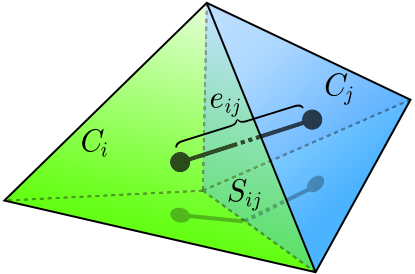
The spatial discretization (mesh), either simplicial (tetrahedra) or regular (cubes), will be denoted $\mathbb{M}$, with $N$ being the number of $n$-dimensional cells $\{C_{i}\}_{i=1,\ldots,N}$ in $\mathbb{M}$. The size of a mesh will refer to the maximum diameter $h$ of its cells. The Lebesgue measure will be denoted by $|.|$. Thus, $|C_{i}|$ is the volume of cell $C_{i}$, $|C_{i}\cap C_{j}|$ is the area of the face common to $C_{i}$ and $C_{j}$, etc (see Figure 2). The dual of $\mathbb{M}$ is the circumentric dual cell complex [28], formed by connecting the circumcenters of each cell $C_{i}$ based on the connectivity of $\mathbb{M}$. We will further assume that the mesh $\mathbb{M}$ is Delaunay with well shaped elements [47] to avoid degeneracies of its orthogonal dual as well as to simplify the exposition. We will also use the term regular grid (or Cartesian grid) to designate a mesh that consists of cells that are $n$-dimensional cubes of equal size. The notation $N(i)$ will denote the set of indices of cells neighboring cell $C_{i}$, that is, cell $C_{i}$ shares a face with cell $C_{j}$ iff $j\in N(i)$. We will say that a pair of cells $C_{i},C_{j}$ is positively oriented around an edge $e$ if they share a face containing $e$ and they are oriented such that they “turn” clockwise around the edge when viewed along the oriented edge. The same term will be used similarly for triplets of cells $C_{i},C_{j},C_{k}$ where $i,k\in N(j)$ and all three cells contain edge $e$.

The notation $(.,.)$ and $\langle.,.\rangle$ will respectively refer to the $L^{2}$ inner product of vectors and the pairing of one-forms and vector fields, while their discrete counterparts will be denoted by $(\!(.,.)\!)$ and $\langle\!\langle.,.\rangle\!\rangle$. Table 1 summarizes the main variables used in the remainder of this paper, along with their meaning and representation.

Suppose that the domain $M$ is approximated by a mesh $\mathbb{M}$. Our first step in constructing a discrete representation of ideal fluids is to approximate ${\rm SDiff}(M)$ with a finite dimensional Lie group in such a way that the elements of the corresponding Lie algebra can be considered as a discretization of divergence-free vector fields. To achieve this goal, we will not discretize the diffeomorphism $g$ itself, but rather the associated operator $U_{g}:L_{2}\rightarrow L_{2}$ defined by $\varphi(x)\mapsto\varphi(g^{-1}(x))$. Here $L^{2}=L^{2}(M,\mathbb{R})$ is the space of square integrable real valued functions on $M$. An important property of $U_{g}$ is given by the following lemma, which follows from the change of variables formula.

Another important property of $U_{g}$ is that it preserves constants, i.e., $U_{g}C=C$ for every constant function $C$, which can be seen as mass preservation for fluids. Next we present an approach to discretize this operator $U_{g}$ while respecting its two defining properties.

We also introduce a discrete approximation of the continuous $L^{2}$ inner product of functions $\langle\varphi,\psi\rangle=\int_{M}\varphi\psi$ through:

In order to better respect the continuous structures at play, we further enforce that our discrete configuration space of diffeomorphisms satisfies two key properties of $U_{g}$: volume-preservation, reflecting the fact that $U_{g}$ is unitary, and total mass preservation, as $U_{g}$ preserves constants. We will thus only consider matrices $q$ that:

• •

  preserve the discrete $L^{2}$ inner product of functions, i.e.,

  $$\langle q\varphi_{h},q\psi_{h}\rangle=\langle\varphi_{h},\psi_{h}\rangle,$$

  where the inner product of discrete functions is defined by Eq. (4). Denoting

  $$\Omega=\begin{pmatrix}|C_{1}|&0&\ldots&0\\ 0&|C_{2}|&\ldots&0\\ \vdots&\vdots&\ddots&\vdots\\ 0&0&\ldots&|C_{N}|\\ \end{pmatrix},$$

  note that this discrete notion of volume preservation directly implies that for our mesh $\mathbb{M}_{h}$ a volume preserving matrix $q$ satisfies

  $$q^{T}\Omega q=\Omega.$$

  The matrix $q$ is thus $\Omega$-orthogonal, restricted to matrices of determinant $1$.

• •

  preserve constant vectors (i.e., vectors having all coordinates equal) as well:

  $$q\mathbf{1}=\mathbf{1},\quad\text{where: }\mathbf{1}=\left(\begin{smallmatrix}1\\ \vdots\\ \\ 1\end{smallmatrix}\right).$$

  The matrix $q$ must thus be signed stochastic as well.

Consequently, the finite dimensional space of matrices we will use to discretize volume-preserving diffeomorphisms has the following definition:

Our finite dimensional configuration space $\mathcal{D}(\mathbb{M})$ for fluid dynamics is thus the intersection of two Lie groups: the $\Omega$-orthogonal group, and the group of invertible stochastic matrices; therefore, it is a Lie group. Note that if all cells of $\mathbb{M}$ have the same volume, i.e., $\Omega=\Omega_{0}\;\mathrm{Id}$, then a matrix $q\in\mathcal{D}(\mathbb{M})$ is orthogonal in the usual sense and the equality (5) implies $\sum_{i}q_{ij}=1$. For such meshes (which include Cartesian grids), the matrix $q$ is signed doubly-stochastic.

Now that we have established a finite dimensional configuration space $\mathcal{D}(\mathbb{M})$, we describe its associated Lie algebra, and show that elements of this Lie algebra provide a discretization of divergence-free vector fields ${\rm SVect}(M)$. We will assume continuous time for simplicity, but a fully discrete treatment of space and time will be introduced in Section 5.

Consider a smooth path in the space of volume-preserving diffeomorphisms $g_{t}\in{\rm SDiff}(M)$ with $g_{0}=\mathrm{Id}$, and let $q_{h}(t)$ be an approximation of $g_{t}$, i.e., for any piecewise constant function $\varphi_{h}^{0}$ approximating a smooth function $\varphi^{0}\in C^{1}(M,\mathbb{R}),$ a discrete version of $\varphi^{0}\circ g^{-1}_{t}=\varphi(t)$ is given by

Assuming $q_{h}(t)$ is smooth in time, we define its Eulerian velocity $A_{h}(t)$ to be

thus yielding

Since $\frac{d}{dt}(\varphi^{0}\circ g^{-1}_{t})=-\langle\mathrm{\mathbf{d}}\varphi(t),v_{t}\rangle=-\mathbf{L}_{v_{t}}\varphi$, where $v_{t}=\dot{g}_{t}\circ g^{-1}_{t}$ and $\mathbf{L}_{v_{t}}$ is the Lie derivative, the matrix $A_{h}(t)$ represents an approximation of the Eulerian velocity field $v_{t}$, which motivates the following definition:

If a curve of matrices $q(t)$ belongs to the configuration space $\mathcal{D}(\mathbb{M})$ (i.e., if $q(t)$ is $\Omega$-orthogonal signed stochastic), then its associated $A$ belongs to its Lie algebra that we denote as $\mathfrak{D}(\mathbb{M})$. Matrices from this Lie algebra inherit the properties that their rows must sum to zero:

and they are $\Omega$-antisymmetric:

These two properties can be intuitively understood as discrete statements that $A$ represents an advection, and the vector field representing this advection is divergence-free. Lie algebra elements for arbitrary simplicial meshes will be called null-row $\Omega$-antisymmetric matrices. Note that if the mesh is regular ($\Omega=\Omega_{0}\;\mathrm{Id}$), $q$ belongs to the orthogonal group and the matrix $A$ has to be antisymmetric with both its rows and columns summing to zero (“doubly null”).

The link between convergence of $A_{h}(t)$ to $\mathbf{L}_{v_{t}}$ and convergence of $q_{h}(t)$ to $U_{g_{t}}$ is described by the following lemma.

A space-discrete flow that approximates a continuous flow $g(t)\in{\rm SDiff}(M)$ is defined to be a smooth path $q(t)\in\mathcal{D}(\mathbb{M})$ in the space of $\Omega$-orthogonal signed stochastic matrices, such that $q(t)\rightsquigarrow g(t)\in{\rm SDiff}(M)$ (see Definition 2) and $A(t)=-\dot{q}(t)\,q^{-1}(t)\rightsquigarrow v_{t}=\dot{g}_{t}(g^{-1}_{t})$ (see Definition 3). It is straightforward to show that the Lie algebra structure of the space of divergence-free vector fields is preserved by our discretization. Indeed, if two matrices $A$ and $B$ approximate vector fields $u$ and $v$ then their commutator $[A,B]$ approximates the commutator of the Lie derivative operators:

Since $\mathbf{L}_{u}\mathbf{L}_{v}-\mathbf{L}_{v}\mathbf{L}_{u}=\mathbf{L}_{[u,v]}$, we obtain $[A,B]\rightsquigarrow[u,v],$ where $[.,.]$ denotes both the commutator of vector fields and the commutator of matrices. This property will be very useful to deal with Lin constraints later on.

For a smooth path $q(t),$ the matrix $A(t)$ describes the infinitesimal exchanges of fluid particles between any pair of cells $C_{i}$ and $C_{j}$. We will thus assume that $A_{ij}$ is non-zero only if cells $C_{i}$ and $C_{j}$ share a common boundary, i.e., are immediate neighbors. This sparsity will be numerically advantageous later on to reduce the computational complexity of the resulting integration schemes. We thus choose to restrict discrete paths $\{q(t)\}$ on $\mathcal{D}(\mathbb{M})$ to those for which $A(t)$ satisfies this constraint²² 2 Although we will adopt this sparsest form of the velocity in this paper, there may be advantages in considering larger non-zero neighborhoods in future work.. In other words, we only consider null-row $\Omega$-antisymmetric matrices satisfying the constraints as valid discrete vector fields. The non-zero elements $A_{ij}$ of these matrices correspond to boundaries between adjacent cells $C_{i}$ and $C_{j}$, and can be interpreted as directional transfer densities (per second) from $C_{i}$ to $C_{j}$—they could abusively be called “fluxes” on regular grids; but we will make the proper link with the integrals of the velocity field over mesh faces in the next section.

More formally, we define the constrained set $S_{q}\subset T_{q}\mathcal{D}(\mathbb{M})$ as the set of matrices corresponding to exchanges between neighboring cells only, i.e., $\dot{q}\in S_{q}$ if and only if $(\dot{q}q^{-1})_{ij}\neq 0$ implies that the cells $C_{i}$ and $C_{j}$ are neighbors. In this case the matrix $A$ is defined by a set of non-zero values $A_{ij}$ defined on faces between adjacent cells $C_{i}$ and $C_{j}$. As mentioned previously, to indicate their adjacency, we will write that $j\!\in\!N(i)$ and $i\!\in\!N(j)$, where $N(k)$ refers to the set of indices of adjacent cells to cell $C_{k}$ in the mesh $\mathbb{M}$. We will say that a matrix $A$ belongs to the class $\mathcal{N}$ if $A_{ij}\neq 0$ implies $j\!\in\!N(i)$. Finally, we will denote by $\mathcal{S}\equiv S_{\text{Id}}=\mathfrak{D}(\mathbb{M})\cap\mathcal{N}$, the constrained set at the identity. Consequently, our treatment of fluid dynamics will only consider matrices $A$ in $\mathcal{S}\subset\mathfrak{D}(\mathbb{M})$, i.e., matrices in $\mathfrak{D}(\mathbb{M})$ satisfying the sparsity constraints.

Note that if two matrices $A$ and $B$ both satisfy the constraints, their commutator need not: while the element of the commutator corresponding to any pair of cells which are more than two cells away is zero, the element $[A,B]_{ij}$ may be non-zero when cells $C_{i}$ and $C_{j}$ are “two cells away” from each other since

Notice that the commutator is zero for neighboring cells since $A_{kk}=B_{kk}=0$ due to their $\Omega$-antisymmetry. Writing $[\mathcal{S},\mathcal{S}]=\{[A,B]\mid A,\,B\in\mathcal{S}\}$, one sees that $\mathcal{S}\cap[\mathcal{S},\mathcal{S}]=\{\mathbf{0}\}$, where $\mathbf{0}$ is the zero matrix. Therefore, the constraints we just defined are non-holonomic.

Suppose we have a family of discrete flows $q_{h}(t)$ which approximates a flow $g_{t}\in{\rm SDiff}(M)$ such that $A_{h}(t)=-\dot{q}_{h}(t)\,{q_{h}(t)}^{-1}$ approximates $\mathbf{L}_{v_{t}}$ and satisfies the NHC. Let’s see how individual elements $(A_{h})_{ij}(t)$ of $A_{h}(t)$ are related to spatial values of $v_{t}$. Recall that

is a discrete version of the advection equation

and $A_{h}(t)\varphi_{h}(t)\to\mathbf{L}_{v_{t}}\varphi$ in the $C^{0}$ norm. But it also means that $(\Omega A_{h}(t)\varphi_{h}(t))_{i}$ is an approximation to the integral $\int_{C_{i}}\mathbf{L}_{v_{t}}\varphi_{t}$, i.e.,

where $\vec{n}$ is the normal vector to the boundary of $C_{i}$ and $(.,.)$ denotes the inner product of vectors. However,

where $S_{ij}$ is the face shared by cells $C_{i}$ and $C_{j}$, and $\vec{n}_{ij}$ the normal vector to $S_{ij}$ oriented from $C_{i}$ to $C_{j}$. By comparing this result to equation (7), it is clear that an element $\Omega_{i}(A_{h})_{ij}(t)$ can be considered (up to a constant) as an approximation to the flux of a vector field $v(t)$ through $S_{ij}$:

We know that $\int_{S_{ij}}(v_{t},\vec{n})\approx(v_{t}(x_{ij}),\vec{n}_{ij})S_{ij}+O(h^{2})$, where $x_{ij}$ is the barycenter of the boundary $S_{ij}$ and $|S_{ij}|$ is the area of $S_{ij}$. Therefore, we obtain that, up to a constant dependent on local mesh measures, $(A_{h})_{ij}$ approximates the flux through the boundary between $C_{i}$ and $C_{j}$, i.e.,

In the case of a Cartesian grid of size $h$ this formula simplifies to:

One of the goals of this paper is to approximate geodesic flows on ${\rm SDiff}(M)$ by Lagrangian flows on $\mathcal{D}(\mathbb{M})$. To achieve this goal, we first need to define a Lagrangian $\mathcal{L}_{h}(q,\dot{q})$ such that

and

Such a Lagrangian, depending only on $A=-\dot{q}q^{-1}$ to mimic the continuous case, can then be used to formulate fluid dynamics through a discrete Lagrange-d’Alembert principle (to account for the non-holonomic constraint we impose on the sparsity of our Eulerian velocity approximation):

Note that the constraint on the variations of $q$ will induce a constraint on the variations of $A$, giving rise to a discrete version of the well-known Lin constraints of the form $\delta A=\dot{B}+[A,B],$ with $B=-\delta q\;q^{-1}$ (see Section 4.2).

However, we will show in later sections that coming up with a proper Lagrangian will require great care. As is typical with nonholonomic systems, the dynamics on $\mathcal{D}(\mathcal{M})$ will depend strongly on the values of $\partial\mathcal{L}_{h}/\partial A$ (i.e., the matrix with $\partial\mathcal{L}_{h}/\partial A_{ij}$ as its $(i,j)$ element) outside of the constraint set $\mathcal{S}$ because of the commutator present in the Lin constraints. In particular, a conventional discretization of the kinetic energy via the sum of all the squared fluxes on the grid would lead to a matrix $\partial\mathcal{L}_{h}/\partial A$ with only values on pairs of adjacent cells, resulting in no dynamics. Instead, the Lagrangian must depend on values $A_{ij}$ where $i\notin N(j)$.

To satisfy properties (8) and (9), we will look for a Lagrangian $\mathcal{L}_{h}$ of the form

where the discrete $L^{2}$-inner-product $(\!(\cdot,\cdot)\!)$ will be defined to satisfy the following properties (where $(\cdot,\!\cdot)$ denotes the continuous inner product of vector fields): for all $A,B\in\mathcal{S}$,

and for all $A,B,C\;\in\mathcal{S}$

where $\flat$ is the continuous flat operator (see for instance [1]). These properties will guarantee that conditions (8) and (9) are satisfied, and will lead to the proper dynamics. In the next section we will present a discretization of differential forms and a few operators acting on them to help us construct the discrete $L^{2}$-inner product (or equivalently, the discrete flat operator $\flat$).

In our context, a discrete $0$-form is a function ${{}^{\scriptscriptstyle 0\!\!}F}$ that is piecewise constant per cell as previously defined in Section 2. Note that its representation is a vector of $N$ cell values,

where ${{}^{\scriptscriptstyle 0\!\!}F}_{i}$ represents the value of the function ${{}^{\scriptscriptstyle 0\!\!}F}$ in cell $C_{i}$. Also, the volume integral of such a discrete $0$-form is obtained by weighting the value of each cell by the Lebesgue measure of this cell, and summing all contributions:

As the space $\mathcal{D}(\mathbb{M})$ of matrices is used to discretize vector fields, a natural way to discretize one-forms is to also use matrices to respect the duality between these two entities. Moreover, it is in line with the previous definition for $0$-forms that were encoded as a 1-tensor: $1$-forms will now be encoded by a $2$-tensor. Notice that this is also reminiscent of the approximation $TM\approx M\times M$ used in discrete mechanics [36].

Therefore, we will assume hereafter that a discrete one-form ${{}^{\scriptscriptstyle 1\!\!}F}$ is defined by an antisymmetric matrix: ${{}^{\scriptscriptstyle 1\!\!}F}\in\mathfrak{so}(N)$.

We extend our definition of one-forms to two-forms in a similar fashion: discrete $2$-forms will be encoded as $3$-tensors ${{}^{\scriptscriptstyle 3\!\!}F}_{ijk}$ that are completely antisymmetric, i.e., antisymmetric with respect to any pair of indices.

References

- [1] Abraham, R., J. E. Marsden, and T. Ratiu [1988] Manifolds, Tensor Analysis, and Applications, Springer (Applied Mathematical Sciences Vol. 75).
- [2] Arnold, V. I., [1966], Sur la géométrie différentielle des groupes de Lie de dimenson infinie et ses applications à l’hydrodynamique des fluides parfaits, Ann. Inst. Fourier, Grenoble, 16:319–361.
- [3] Arnold, V. I., [1969], Hamiltonian character of the Euler equations of the dymnamics of solids and of an ideal fluid, Uspekhi Mat. Nauk, 24:225–226.
- [4] Arnold, D.N., R. S. Falk, and R. Winther [2006], Finite element exterior calculus, homological techniques, and applications, Acta Numerica, 15, 1–155.
- [5] Arnold, V. I. and B. Khesin [1992], Topological methods in hydrodynamics, Ann. Rev. Fluid Mech., 24, 145–166.
- [6] Arnold, V. I. and B. Khesin [1998], Topological methods in hydrodynamics, Springer-Verlag.
- [7] Bochev, P. B. and J. M. Hyman [2005], Principles of mimetic discretizations of differential operators, Preprint LA-UR-05- 4244.
- [8] Bossavit, A. [1998],Computational Electromagnetism. Academic Press (Boston).
- [9] Brenier, Y. [1989], The least action principle and the related concept of generalized flows for incompressible perfect fluids, J. Amer. Math. Soc. 2, no. 2, 225–255.
- [10] Brenier, Y. [1991], Polar factorization and monotone rearrangement of vector-valued functions, Comm. Pure Appl. Math. 44(4), 375–417.
- [11] Brenier, Y. [1999], Minimal geodesics on groups of volume-preserving maps and generalized solutions of the Euler equations, Comm. Pure Appl. Math. 52, 411–452.
- [12] Bretherton, F. P. [1970], A note on Hamilton’s principle for perfect fluids, J. Fluid Mech. 44, 99–31.
- [13] Cendra, H. and J. E. Marsden [1987], Lin constraints, Clebsch potentials and variational principles, Physica D 27, 63–89.
- [14] Cotter, C. J. and D. D. Holm [2009], Continuous and Discrete Clebsch Variational Principles, Foundations of Computational Mathematics 9(2), 221–242.
- [15] Cotter, C. J., D. D. Holm, and P. E. Hydon [2007], Multisymplectic formulation of fluid dynamics using the inverse map, Proc. Roy. Soc. A 463, 2671–2688.
- [16] Dellnitz, M., A. Hohmann, O. Junge, and M.Rumpf [1997], Exploring invariant sets and invariant measures, CHAOS: An Interdisciplinary Journal of Nonlinear Science 7(2), 221–228.
- [17] Desbrun, M., E. Kanso, and Y. Tong, [2005], Discrete differential forms for computational modeling. Chapter in ACM SIGGRAPH Course Notes on Discrete Differential Geometry.
- [18] Desbrun, M., A. N. Hirani, and J. E. Marsden [2003], Discrete exterior calculus for variational problems in computer vision and graphics, Proc. CDC 42, 533–538.
- [19] DiPerna, R. G. and A. G. Majda [1987], Oscillations and concentrations in weak solutions of the incompressible fluid equations, Math. Physics 108, 667–689.
- [20] Duponcheel, M., P. Orlandi, and G. Winckelmans [2008], Time-reversibility of the Euler equations as a benchmark for energy conserving schemes, Journal of Computational Physics 227 19, 8736–8752.
- [21] Harlow, F. H. and J. E. Welch [1965], Numerical calculation of time-dependent viscous incompressible flow of fluid with free surface, Physics of Fluids 8(12), 2182–2189.
- [22] Ebin, D. G. and J. E. Marsden [1970], Groups of diffeomorphisms and the motion of an incompressible fluid, Ann. of Math., 92, 102–163.
- [23] Elcott, S., Y. Tong, E. Kanso, P. Schröder, and M. Desbrun [2007], Stable, circulation-preserving simplicial fluids, ACM Transactions on Graphics, 26(1), Art. 4.
- [24] Gresho, P. M. and R. L. Sani [2000], Incompressible Flow and the Finite Element Method, J. Wiley & Sons.
- [25] Hairer, E., C. Lubich, and G. Wanner [2006],Geometric Numerical Integration: Structure-Preserving Algorithms for Ordinary Differential Equations. Springer-Verlag.
- [26] Haker, S., L. Zhu, A. Tannenbaum, and S. Angenent [2004], Optimal Mass Transport for Registration and Warping, International Journal on Computer Vision 60(3), 225–240.
- [27] Hou, T. Y. and Z. Lei [2009], On the Stabilizing Effect of Convection in 3D Incompressible Flow, Commun. Pure Appl. Math., 62(4), 501–564.
- [28] Hirani, A. [2003], Discrete Exterior Calculus, PhD thesis, California Institute of Technology.
- [29] Koopman, B. O. [1931], Hamiltonian Systems and Transformations in Hilbert Spaces, Proc. Nat. Acad. Sci. (USA), 17, 315–318.
- [30] LeVeque, R.J. [2002], Finite Volume Methods for Hyperbolic Problems , Cambridge University Press.
- [31] Mahesh, K., G. Constantinescu, and P. Moin [2004], A numerical method for large-eddy simulation in complex geometries, J. Comput. Phys. 197, 1, 215–240.
- [32] Marsden, J. E. and T. S. Ratiu [1999], Introduction to Mechanics and Symmetry, 17 of Texts in Applied Mathematics, vol. 17; 1994, Second Edition, 1999. Springer-Verlag.
- [33] Marsden, J. E., T. S. Ratiu, and S. Shkoller [2000], The geometry and analysis of the averaged Euler equations and a new diffeomorphism group, Geom. Funct. Anal., 10(3), 582–599.
- [34] Marsden, J. E. and J. Scheurle [1993], The reduced Euler-Lagrange equations, Fields Institute Comm., 1, 139–164.
- [35] Marsden, J. E. and A. Weinstein [1983], Coadjoint orbits, vortices and Clebsch variables for incompressible fluids, Physica D 7, 305–323.
- [36] Marsden, J. E. and M. West [2001], Discrete mechanics and variational integrators, Acta Numerica, 10, 357–515.
- [37] Mullen, P., K. Crane, D. Pavlov, Y. Tong, M. Desbrun [2009], Energy-preserving integrators for fluid simulation, ACM Trans. on Graphics 28(3), Art. 38.
- [38] Munkres, J. R. [1984], Elements of Algebraic Topology, Addison-Wesley, Menlo Park, CA.
- [39] Newcomb, W. A. [1962], Lagrangian and Hamiltonian methods in Magnetohydrodynamics, Nuc. Fusion Suppl. part 2, 451–463.
- [40] Perot, B. [2000], Conservation properties of unstructured staggered mesh schemes, J. Comput. Phys. 159, 1, 58–89.
- [41] Salmon, R. [2004], Poisson-Bracket Approach to the Construction of Energy and Potential-Enstrophy Conserving Algorithms for the Shallow-Water Equations, J. Atmos. Sci., 61, 2016–2036.
- [42] Sen, S., S. Sen, J. C. Sexton, and D. H. Adams [2000], Geometric discretization scheme applied to the abelian Chern-Simons theory, Phys. Rev. E 61(3), 3174–3185.
- [43] Simo, J.C., and F. Armero [2000], Unconditional stability and long-term behavior of transient algorithms for the incompressible Navier-Stokes and Euler equations, Computer Methods in Applied Mechanics and Engineering 111, 111–154.
- [44] Shnirelman, A. I. [1994], Generalized fluid flows, their approximation and applications, Geom. and Funct. Analysis, 4, no. 5, 586–620.
- [45] Shnirelman, A. I. [1997], On the non-uniqueness of weak solution of the Euler equations, Comm. Pure Appl. Math. 50(12), 1261–1286.
- [46] Stern, A., Y. Tong, M. Desbrun, and J. E. Marsden [2008], Variational Integrators for Maxwells Equations with Sources, Progress in Electromagnetics Research Symposium (PIERS) 4(7), 711–715.
- [47] Tournois, J., C. Wormser, P. Alliez, M. Desbrun [2009], Interleaving Delaunay Refinement and Optimization for Practical Isotropic Tetrahedron Mesh Generation, ACM Trans. on Graphics 28(3), Art. 75.