Numerical Evaluation Of the Oscillatory Integral over $\exp(i\pi x)x^{1/x}$ between 1 and Infinity

Richard J. Mathar URL: http://www.strw.leidenuniv.nl/˜mathar Email address: mathar@strw.leidenuniv.nl Address: Leiden Observatory, Leiden University, P.O. Box 9513, 2300 RA Leiden, The Netherlands

Date: August 24, 2026

Abstract.

Real and imaginary part of the limit $2N\to\infty$ of the integral $\int_{1}^{2N}\exp(i\pi x)\sqrt[x]{x}dx$ are evaluated to 20 digits with brute force methods after multiple partial integration, or combining a standard Simpson integration over the first half wave with series acceleration techniques for the alternating series co-phased to each of its points. The integrand is of the logarithmic kind; its branch cut limits the performance of integration techniques that rely on smooth higher order derivatives.

Key words and phrases:

Oscillatory Integral, Filon Quadrature, Incomplete Gamma Function

2010 Mathematics Subject Classification

Primary 65D30, 65B05; Secondary 40A25, 65T40

1. Scope

1.1. M. R. Burns’ Constant

Definition 1.

The MRB constant is the sum of the series [18, A037077]

(1)

M\equiv\lim_{N\to\infty}\sum_{n=1}^{2N}(-1)^{n}\sqrt[n]{n}=\sum_{k=1}^{\infty}(-1)^{k}(k^{1/k}-1)\approx 0.18785964.

Direct summation of the alternating series is slow and generates roughly 3 valid digits after ten thousand terms (Table 1). Euler summation [1, (3.6.27)][10] is successful in accelerating the convergence, witnessed in Table 2.

Table 1. Partial sums of (1) as a function of the upper limit of summation.

$\hat{k}$	$\sum_{k=1}^{\hat{k}}(-1)^{k}(k^{1/k}-1)$
$10$	0.313231759254…
$10^{2}$	0.211329543346…
$10^{3}$	0.191323989712…
$10^{4}$	0.188320351076…
$10^{5}$	0.187917210140…

Table 2. Approximations to (1) after Euler resummation of the first

\hat{k}

terms.

$\hat{k}$	$E(1)$
10	0.187885886113800730351382438464680824292327407645248188116946…
20	0.187859649854050194658445181421685949965109596411421113134589…
40	0.187859642462068655529781630996634559217485607603915205816966…
100	0.187859642462067120248517934054273314215151463271236583869269…
200	0.187859642462067120248517934054273230055903094900138786171982…

More efficient methods lead to even quicker convergence, as demonstrated in Table 3. An accuracy of 60 digits is reached after 100 terms and will be sufficient for all purposes of this script.

Table 3. Approximations to (1) with the first Cohen-Villegas-Zagier algorithm using terms up to

\hat{k}

[3].

$\hat{k}$	$M$
10	0.187859642389333316567457476113016727048599369932998191180459…
20	0.187859642462067119674255755542940758484982176117045969528027…
40	0.187859642462067120248517934054273140023454509840554949525330…
100	0.187859642462067120248517934054273230055903094900138786171986…

1.2. Oscillatory Integral

The integrated analog of the series is a complex-valued integral of oscillatory character, which is difficult to evaluate by direct integration if the upper limit becomes large, illustrated by Figure 1.

Definition 2.

(Sequence of oscillatory integrals)

(2)

I(2N)\equiv\int_{1}^{2N}(-1)^{x}\sqrt[x]{x}dx=\int_{1}^{2N}e^{i\pi x}x^{1/x}dx,\quad N\in\mathbb{Z}.

Not convergent in the continuum limit at $N\to\infty$ , the limit of the sequence of integrals with an integral difference in the upper limits $2N$ exists. The objective of this work is to evaluate this limit $M_{I}$ .

Definition 3.

(Ultraviolet limit of the sequence)

(3)

M_{I}\equiv\lim_{N\to\infty}I(2N).

Remark 1.

The absolute value $|M_{I}|\approx 0.6876523689$ is close to $M+\frac{1}{2}$ [18, A157852]. Changing the upper limit to $2N+1$ increases $M_{I}$ by $2i/\pi$ .

Refer to caption — Figure 1. Real and imaginary part of $e^{i\pi x}x^{1/x}$ , the integrand in (2).

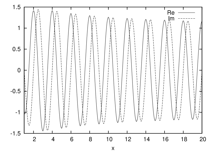
To compute $M_{I}$ , the manuscript looks at repeated partial integration to quench the integrand at large $x$ in preparation for standard methods of sampling along the abscissa (Sections 2.1 and 2.2), investigates splitting the integral into an alternating series and a base interval (Section 2.3), expansion of $x^{1/x}$ into a series over $(\log x/x)^{n}$ (Section 2.4), changing the path of integration in the complex plane (Section 2.5), and considers reverse application of the Euler-Maclaurin integral formula (Appendix C).

2. Numerical Analysis

2.1. Iterated Partial Integration

A partial integration of (2) yields

(4)

\int_{1}^{2N}e^{i\pi x}x^{1/x}dx=-\frac{i}{\pi}e^{i\pi x}x^{1/x}\bigg|_{1}^{2N}+\frac{i}{\pi}\int_{1}^{2N}e^{i\pi x}x^{1/x}\frac{1-\log x}{x^{2}}dx.

The limit $N\to\infty$ can be performed in the pre-integrated term,

(5)

M_{I}=-\frac{2i}{\pi}+\frac{i}{\pi}\int_{1}^{\infty}e^{i\pi x}x^{1/x}\frac{1-\log x}{x^{2}}dx,

which essentially compresses the oscillations with a factor $\propto\log(x)/x^{2}$ , as shown in Figure 2.

A second partial integration of (5) may follow,

(6)

\int_{1}^{2N}e^{i\pi x}x^{1/x}\frac{1-\log x}{x^{2}}dx\\ =-\frac{i}{\pi}e^{i\pi x}x^{1/x}\frac{1-\log x}{x^{2}}\Big|_{1}^{2N}+\frac{i}{\pi}\int_{1}^{2N}e^{i\pi x}x^{1/x}\frac{1-3x+2(x-1)\log(x)+\log^{2}x}{x^{4}}dx

with the limit

(7)

M_{I}=-\frac{2i}{\pi}+\frac{1}{\pi^{2}}-\frac{1}{\pi^{2}}\int_{1}^{\infty}e^{i\pi x}x^{1/x}\frac{1-3x+2(x-1)\log(x)+\log^{2}x}{x^{4}}dx.

Repeating, a simple scheme for the $n$ -th derivative of the base function $f$ ,

(8)

f^{(0)}(x)\equiv x^{1/x};\quad f^{(n+1)}(x)\equiv\frac{d}{dx}f^{(n)}(x),

can be phrased as a set of coefficients $\alpha$ ,

(9)

f^{(n)}(x)\equiv x^{1/x}\sum_{r,s\geq 0}\alpha_{n,r,s}\frac{\log^{s}(x)}{x^{r}}.

Explicit computation with the chain rule establishes the recurrence

(10)

\alpha_{n+1,r,s}=\alpha_{n,r-2,s}-\alpha_{n,r-2,s-1}+(s+1)\alpha_{n,r-1,s+1}-(r-1)\alpha_{n,r-1,s}.

The initial conditions are

(11)

\alpha_{n,r,s}=0\quad\text{if}\quad r<0\quad\text{or}\quad s<0;\quad\alpha_{0,0,0}=1.

Equations (5), (7) and the representation through $n$ -fold partial integration are summarized with

(12)

M_{I}=b(n)+\left(\frac{i}{\pi}\right)^{n}\int_{1}^{\infty}e^{i\pi x}f^{(n)}(x)dx,

defining pre-integrated terms

(13)

b(n+1)=b(n)-\frac{i}{\pi}f^{(n-1)}(1);\quad b(0)=0;\quad b(1)=-\frac{2i}{\pi}.

The infinite interval from 1 to $\infty$ can be mapped onto the interval from 0 to $1/2$ with the substitution (one of a family of rational maps)

(14)

y=\frac{1}{1+x};\quad x=\frac{1}{y}-1;\quad dx=-\frac{dy}{y^{2}};

(15)

\int_{1}^{\infty}e^{i\pi x}f^{(n)}(x)dx=\int_{0}^{1/2}e^{i\pi x(y)}f^{(n)}(x(y))\frac{dy}{y^{2}}.

A combination of (12) and (15) yields:

Algorithm 1.

Compute $M_{I}$ with a Simpson integration on $s$ points in the interval $0\leq y\leq 1/2$ :

(16)

M_{I}=b(n)+\left(\frac{i}{\pi}\right)^{n}\int_{0}^{1/2}e^{i\pi x(y)}f^{(n)}(x(y))\frac{dy}{y^{2}}.

Table 4 illustrates that a choice of $n$ near 5 or 6 yields optimum convergence (because $b(n)$ then approximate $M_{I}$ best), and that integration with $s\approx 60\,000$ abscissa points generates of the order of 13 valid digits. Note that Romberg (Richardson) extrapolation with the standard $15:1$ weighting of step width halving does not work as the integrand is not in the polynomial class.

Table 4. Algorithm 1: Simpson integration with

s

points in the interval

0\leq y\leq 1/2

and the

n

-th partial integration (12) inserted in (15).

$n$	$s$	$\Re(M_{I})$	$\Im(M_{I})$
2	2000	0.07077873792033467823	-0.68400849330911320239
2	4000	0.07077826545794147869	-0.68400115445281602856
3	2000	0.07077594388618778878	-0.68400039709147911789
3	4000	0.07077603597753547955	-0.68400040477320427448
3	8000	0.07077604728595562114	-0.68400040978725640089
3	16000	0.07077604069379310873	-0.68400038906169127559
3	32000	0.07077603794889411182	-0.68400038968332537849
3	64000	0.07077603964902400034	-0.68400038933267435379
5	2000	0.07077603934743949117	-0.68400038942675266591
5	4000	0.07077603931081786932	-0.68400038943414042302
5	8000	0.07077603931077043492	-0.68400038943655207372
5	16000	0.07077603931149307863	-0.68400038943803823084
5	32000	0.07077603931155557088	-0.68400038943794081422
5	64000	0.07077603931152496616	-0.68400038943793426656
6	2000	0.07077603931115051881	-0.68400038943952383435
6	4000	0.07077603931156321151	-0.68400038943794556862
6	8000	0.07077603931154254337	-0.68400038943792386069
6	16000	0.07077603931152730519	-0.68400038943793206498
6	32000	0.07077603931152869782	-0.68400038943793231267
6	64000	0.07077603931152878997	-0.68400038943793211168
8	2000	0.07077603932853563807	-0.68400038944555242777
8	4000	0.07077603931259171964	-0.68400038943840850746
9	2000	0.07077603925904942234	-0.68400038951437536286
9	4000	0.07077603930824878310	-0.68400038944270983422

Remark 2.

In a variant of this mapping on a finite interval, the transformation $x=1/u$ in the $n$ -th partial integration yields

(17)

M_{I}=b(n)+(i/\pi)^{n}\int_{0}^{1}e^{i\pi/u}f^{(n)}(1/u)\frac{du}{u^{2}}.

The precision is worse than with Algorithm 1 by approximately one digit. I have not looked into advanced schemes for this type of oscillatory integrals [7, 11] or Sidi’s generalized methods of extrapolation.

2.2. Exponential Scaling

A characteristic of Algorithm 1 is that the integrand is basically reduced by another factor $1/x$ for each additional partial integration. The variable transformation $\log x=z$ , $x=e^{z}$ , $dx=e^{z}dz$ , helps to achieve exponential scaling as the integration variable heads towards infinity, at the cost of an irregular chirp factor in the complex exponential:

(18)

F_{m}=\int_{m}^{\infty}e^{i\pi x}x^{1/x}\frac{1-\log x}{x^{2}}dx=\int_{\log m}^{\infty}(1-z)e^{i\pi\exp(z)}e^{z\exp(-z)-z}dz.

Based on

(19)

\int e^{i\pi\exp(z)+z}dz=-\frac{i}{\pi}e^{i\pi\exp(z)},

and “borrowing” a factor $e^{z}$ in (18) in the integrand,

(20)

F_{m}=\int_{\log m}^{\infty}(1-z)e^{i\pi\exp(z)+z}e^{z\exp(-z)-2z}dz,

a partial integration generates

(21)

F_{m}=\frac{i(-)^{m}}{\pi}\sqrt[m]{m}\frac{1-\log m}{m^{2}}+\frac{i}{\pi}\int_{\log m}^{\infty}e^{i\pi\exp(z)}e^{z\exp(-z)-2z}\left[2z-3+e^{-z}(1-2z+z^{2})\right]dz.

Alternatively, this results applying the substitution $\log x=z$ to (12). After this scheme of partial integrations has been repeated $n$ times, the non-oscillating exponential factor in the integrand is $\exp[z\exp(-z)-(n+1)z]$ .

Algorithm 2.

Perform $n$ partial integrations of (18), then use another transformation $u=e^{-z}$ , $z=-\log u$ to map the range $0\leq z\leq\infty$ to $0\leq u\leq 1$ in the remaining integral, and integrate this over $u$ with a Simpson method. Eventually insert this $F_{1}$ in

(22)

M_{I}=-\frac{2i}{\pi}+\frac{i}{\pi}F_{1}

as seen in (5).

Table 5. Convergence of Algorithm 2: integration of the

n

-th partial integration of

F_{1}

with

s

equidistant points in the interval

0\leq u\leq 1

$n$	$s$	$\Re(M_{I})$	$\Im(M_{I})$
2	4000	0.07077612979610666804	-0.68400038256040301228
2	8000	0.07077604264870771610	-0.68400037471801246748
3	4000	0.07077603954212465077	-0.68400039095784542350
3	8000	0.07077603950170386538	-0.68400038943798882953
4	4000	0.07077603927887287271	-0.68400038944795068337
4	8000	0.07077603931218586254	-0.68400038944147410684
5	4000	0.07077603931112220214	-0.68400038943707487961
5	8000	0.07077603931144862845	-0.68400038943795645974
5	16000	0.07077603931151256105	-0.68400038943794236597
5	32000	0.07077603931153004386	-0.68400038943793234690
5	64000	0.07077603931152889348	-0.68400038943793195977
6	4000	0.07077603931156163745	-0.68400038943790335638
6	8000	0.07077603931152840681	-0.68400038943792930582
6	16000	0.07077603931152865655	-0.68400038943793183965
6	32000	0.07077603931152880374	-0.68400038943793214262
6	64000	0.07077603931152880496	-0.68400038943793212992
6	128000	0.07077603931152880345	-0.68400038943793212926
6	256000	0.0707760393115288035480930	-0.6840003894379321291922485
6	512000	0.0707760393115288035386982	-0.6840003894379321291820339
6	1024000	0.0707760393115288035395359	-0.6840003894379321291828037
6	2048000	0.0707760393115288035395336	-0.6840003894379321291827445
8	4000	0.07077603931135483266	-0.68400038943809843545
8	8000	0.07077603931151793368	-0.68400038943794252308
9	4000	0.07077603931088567214	-0.68400038943711147080
9	8000	0.07077603931148860789	-0.68400038943788083818

An accuracy of $10^{-21}$ can be reached sampling two million points (Table 5) and is reported in the summary. Comparison with Table 4 shows that one to two digits are gained relative to Algorithm 1.

2.3. Longman’s Method

An integral $F$ with an undulating trigonometric factor multiplied by a monotonous $g(x)$ may be split into an integral over the half period with an alternating series attached to each point in that interval [14, 13, 5].

(23)

F_{m}=\int_{m}^{\infty}e^{i\pi x}g(x)dx=\sum_{l\geq 0}\int_{0}^{1}e^{i\pi(m+l+y)}g(m+l+y)dy\\ =(-)^{m}\int_{0}^{1}e^{i\pi y}\sum_{l\geq 0}(-)^{l}g(m+l+y)dy.

The $l$ -series is only alternating if the function $g(x)$ is monotonous and does not change sign. In addition, Euler resummation assumes that the series converges. With $M_{I}$ , $x^{1/x}$ has a maximum at $x=e$ , so we integrate over $1\leq x\leq 3$ with any other method, setting $m=3$ , and relay by one partial integration, $g(x)=f^{(1)}(x)$ , to feature a $g(x)$ that has a single sign with decreasing $|g^{\prime}(x)|$ in $[m,\infty)$ .

Algorithm 3.

Compute $M_{I}$ by Filon-Simpson-integration of $F_{m}$ in (23) over the interval $0\leq y\leq 1$ (Appendix A) and

(24)

M_{I}=\int_{1}^{m}e^{i\pi x}x^{1/x}dx+\frac{i}{\pi}\left[(-)^{m}m^{1/m}-1\right]+\frac{i}{\pi}F_{m};\quad g(x)=x^{1/x}\frac{1-\log x}{x^{2}};\quad(m=3).

With this choice, $g(x)$ has a maximum near $x=4.3$ , associated with the zero of $f^{(2)}(x)$ , which (after detailed inspection) does not destroy the alternating property—if higher order $f^{(n)}(x)$ were employed, $m$ would have to be chosen differently.

Table 6. Convergence of Algorithm 3 with a Simpson integration on

n

abscissa points over

[0,1]

, truncating the alternating series after the

l

-th term followed by extrapolation [3].

$n$	$l$	$\Re(M_{I})$	$\Im(M_{I})$
32	60	0.07077603721021819390	-0.68400038753980049654
32	70	0.07077603721021819390	-0.68400038753980049654
64	70	0.07077603918043104863	-0.68400038931936816305
128	70	0.07077603930333884842	-0.68400038943052296458
256	70	0.07077603931101698843	-0.68400038943746907333
512	70	0.07077603931149681599	-0.68400038943790318846
1024	70	0.07077603931152680433	-0.68400038943793032039
2048	70	0.07077603931152867859	-0.68400038943793201613
4096	70	0.07077603931152879573	-0.68400038943793212212
8192	50	0.07077603931152880305	-0.68400038943793212874
8192	60	0.07077603931152880305	-0.68400038943793212874
16384	50	0.07077603931152880351	-0.68400038943793212916
16384	60	0.07077603931152880351	-0.68400038943793212916

The speed of convergence of the method is demonstrated with Table 6. As the number of evaluations of $g$ is the product of $n$ and $l$ , it turns out effectively to be slower than Algorithm 2.

2.4. Taylor Series the Logarithmic Term

The most advanced method expands the non-oscillatory term of (2) into the Taylor series of the exponential:

Algorithm 4.

(Logarithmic expansion of $x^{1/x}$ )

(25)

\int_{1}^{2N}e^{i\pi x}x^{1/x}dx=\int_{1}^{2N}e^{i\pi x}e^{\frac{1}{x}\log x}dx=\int_{1}^{2N}e^{i\pi x}[1+\sum_{n\geq 1}\frac{1}{n!}\frac{\log^{n}x}{x^{n}}]dx\\ =-\frac{2i}{\pi}+\sum_{n\geq 1}\frac{1}{n!}\int_{1}^{2N}e^{i\pi x}\frac{\log^{n}x}{x^{n}}dx.

The integrals are the $V(\pi,n,n)$ defined in equation (31) in Appendix B. Summing over values taken from Tables 9–11 produces Table 7.

Table 7. Convergence of the partial sum of Algorithm 4.

$\max n$	$\Re(M_{I})$	$\Im(M_{I})$
1	0.05762490298863188764	-0.68331060191932132015
2	0.06935454902524610824	-0.68451362283943263006
3	0.07066781734932533318	-0.68408393964817446557
4	0.07076978736326279015	-0.68400839361204835470
5	0.07077575770475264223	-0.68400096184084805332
6	0.07077602957520227166	-0.68400042266805241181
7	0.07077603908225272182	-0.68400039107408096452
8	0.07077603931050590528	-0.68400038950815469850
9	0.07077603931177817100	-0.68400038944060977421

An accuracy of $10^{-19}$ in real and imaginary part of $M_{I}$ requires summation up to $n=15$ —an estimation derived from results of Remark 4—, and has not been worked out.

2.5. Contour Deformation

The path of the integration may be deformed to a straight line (hypotenuse) from $z=1$ to $z=2N(1+\tau i)$ with adjustable slope $\tau>0$ towards the real axis, and a straight line (short leg) parallel to the imaginary axis back to $2N$ on the real axis. The contribution of $\Im z$ to $\exp(i\pi z)$ leads to a exponential reduction of the integrand as the distance to the real axis grows. (More complicated paths appear not to be more efficient.) The short leg of this triangle contributes

(26)

\lim_{N\to\infty}\int_{2N(1+\tau i)}^{2N}e^{i\pi z+\log z/z}dz=-\frac{i}{\pi}

to the integral.

Algorithm 5.

Compute

(27)

M_{I}=-\frac{i}{\pi}+\lim_{N\to\infty}\int_{1}^{2N(1+\tau i)}e^{i\pi z+\log z/z}dz

with a Simpson integration on $s$ points $z_{j}=1+j(1+\tau i)\Delta t$ , $j=0,\ldots s$ .

Table 8. Algorithm 5: Simpson integration along the line from

z=1

z=2N(1+\tau i)

with

s

abscissa points.

$s$	$N$	$\tau$	$\Re(M_{I})$	$\Im(M_{I})$
64000	20	0.1	0.07077602653194263984	-0.68400205509417633076
64000	20	0.2	0.07077603931143220832	-0.68400038944591701234
64000	20	0.3	0.07077603931156096762	-0.68400038943797230450
128000	20	0.3	0.07077603931153081310	-0.68400038943793467559
256000	20	0.3	0.07077603931152892845	-0.68400038943793232378
64000	40	0.1	0.07077603931142945824	-0.68400038944426949930
128000	40	0.1	0.07077603931149682353	-0.68400038944357500783
64000	40	0.2	0.07077603931176127606	-0.68400038943868543692
128000	40	0.2	0.07077603931154333296	-0.68400038943797921085
64000	80	0.1	0.07077603931041311002	-0.68400038945008174688
128000	80	0.1	0.07077603931145906913	-0.68400038943869147372
256000	80	0.1	0.07077603931152444508	-0.68400038943797958811
64000	80	0.2	0.07077603931534354347	-0.68400038945029316088
128000	80	0.2	0.07077603931176721758	-0.68400038943870468984
256000	80	0.2	0.07077603931154370430	-0.68400038943798041416
512000	80	0.2	0.07077603931152973483	-0.68400038943793514699
1024000	80	0.2	0.07077603931152886174	-0.68400038943793231779
128000	160	0.1	0.07077603931039901029	-0.68400038945023529554
256000	160	0.1	0.07077603931145818783	-0.68400038943870107039
128000	160	0.15	0.07077603931285988807	-0.68400038945052460466
256000	160	0.15	0.07077603931161199070	-0.68400038943871915335
512000	160	0.15	0.07077603931153400264	-0.68400038943798131810

The dependence on three configuration parameters makes quality assessment more difficult than with the other methods, illustrated by Table 8. The contribution missing for any finite $N$ is estimated by

(28)

\int_{2N(1+\tau i)}^{\infty}e^{i\pi z+\log z/z}dz\approx\int_{2N(1+\tau i)}^{\infty}e^{i\pi z}dz=\frac{i}{\pi}e^{2\pi iN(1+i\tau)},

which serves as a guideline how large $\tau$ ought be made given a targeted accuracy and an upper limit $N$ .

3. Summary

The value of $M_{I}$ is

(29)

\lim_{N\to\infty}\int_{1}^{2N}e^{i\pi x}x^{1/x}dx\\ \approx 0.0707760393115288035395-0.68400038943793212918i.

The integral features highly oscillatory behavior and a logarithmic factor in the main integrand, which sets up an interesting test case outside the range of methods that assume “nice” analytic properties in the complex plane.

Appendix A Filon-Simpson Rule

The Simpson rule of integration of a function $G(y)$ is an interpolation between three abscissa points $(y_{0},G(0))$ , $(y_{1},G(1))$ and $(y_{2},G(2))$ by a quadratic polynomial in $y$ [1, (25.2.1)],

G_{m}(y)=\frac{(y-y_{1})(y-y_{2})}{(y_{0}-y_{1})(y_{0}-y_{2})}G(0)+\frac{(y-y_{0})(y-y_{2})}{(y_{1}-y_{0})(y_{1}-y_{2})}G(1)+\frac{(y-y_{0})(y-y_{1})}{(y_{2}-y_{0})(y_{2}-y_{1})}G(2)

followed by integration of this polynomial in the limits $y_{0}\leq y\leq y_{2}$ . A refinement in our case, based on the same quadratic interpolation, is

(30)

\int_{y_{0}}^{y_{0}+2h}e^{i\pi y}G_{m}(y)dy=\frac{ie^{y_{0}\pi i}}{2h^{2}\pi^{3}}[-2+2h^{2}\pi^{2}-3ih\pi+(2-h\pi i)e^{2i\pi h}]G(0)\\ -\frac{2e^{y_{0}\pi i}}{h^{2}\pi^{3}}[-i+h\pi+(i+h\pi)e^{2i\pi h}]G(1)\\ -\frac{ie^{y_{0}\pi i}}{2h^{2}\pi^{3}}[2+h\pi i+(-2+2h^{2}\pi^{2}+3ih\pi)e^{2i\pi h}]G(2),

supposing equidistant abscissa points $y_{1}=y_{0}+h$ and $y_{2}=y_{0}+2h$ . This explicit recognition of the exponential factor gains roughly one additional digit in accuracy in Table 6 compared to the evaluation with $e^{i\pi y}$ incorporated in the value of $G$ .

Appendix B Fichtenholz Integrals

B.1. Fundamental Form

In this appendix, a set of integrals $V(a,k,s)$ is targeted as an aid to Algorithm 4. This is basically evaluating the generalized integro-exponential function [16, 12] for a complex-valued parameter $z=-ia$ .

Definition 4.

(Generalized Integro-Exponential Function)

(31)

V(a,k,s)\equiv\int_{1}^{\infty}e^{iax}\frac{\log^{k}x}{x^{s}}dx.

Remark 3.

There are three simple extensions:

•

Cases with a scaling factor $b$ in the logarithm can be reduced to this fundamental form by binomial expansion of $(\log b+\log x)^{k}$ ,

(32)

\int_{1}^{\infty}e^{iax}\frac{\log^{k}(bx)}{x^{s}}dx=\sum_{l=0}^{k}\binom{k}{l}\log^{k-l}(b)\,V(a,l,s).

•

Reading

(33)

\int_{1}^{\infty}e^{iax}\frac{\log^{k}(bx)}{x^{s}}dx=b^{s-1}\int_{b}^{\infty}e^{iax/b}\frac{\log^{k}y}{y^{s}}dy,

(obtained through the substitution $bx\to y$ ) from right to left shows that other lower limits than 1 are also accessible once the $V$ are known for general $a$ .

•

Integer powers of sines or cosines at the place of the exponential lead back to the fundamental form via Euler’s formula:

(34)		$\displaystyle\int_{1}^{\infty}\sin^{m}(ax)\frac{\log^{k}x}{x^{s}}dx=\frac{1}{(2i)^{m}}\sum_{l=0}^{m}\binom{m}{l}(-1)^{l}V[a(m-2l),k,s];$
(35)		$\displaystyle\int_{1}^{\infty}\cos^{m}(ax)\frac{\log^{k}x}{x^{s}}dx=\frac{1}{2^{m}}\sum_{l=0}^{m}\binom{m}{l}V[a(m-2l),k,s].$

Real and imaginary part of the value $V(a,1,1)$

(36)

\int_{1}^{\infty}e^{iax}\frac{\log x}{x}dx=\int_{1}^{\infty}\cos(ax)\frac{\log x}{x}dx+i\int_{1}^{\infty}\sin(ax)\frac{\log x}{x}dx

are computed separately. The imaginary part is

(37)

\int_{1}^{\infty}\sin(ax)\frac{\log x}{x}dx=\int_{0}^{\infty}\sin(ax)\frac{\log x}{x}dx-\int_{0}^{1}\sin(ax)\frac{\log x}{x}dx

with one constituent [9, (4.421.1)][4, (865.63)][6]

(38)

\int_{0}^{\infty}\sin(ax)\frac{\log x}{x}dx=-\frac{\pi}{2}(\gamma+\log a)\approx-2.704825746060380848849568\quad(a=\pi).

The integral over $[0,1]$ is evaluated by Taylor expansion of the sine which leads to the well converging representation

(39)

\int_{0}^{1}\sin(ax)\frac{\log x}{x}dx=-a\sum_{n\geq 0}(-1)^{n}\frac{a^{2n}}{(2n+1)!(1+2n)^{2}}\\ =-a\,_{2}F_{3}\left(\begin{array}[]{c}1/2,1/2\\ 3/2,3/2,3/2\end{array}\mid-\frac{a^{2}}{4}\right)\approx-2.6581349165086\quad(a=\pi).

The difference between this value and (38) represents (37),

(40)

\int_{1}^{\infty}\sin(ax)\frac{\log x}{x}dx=-\frac{\pi}{2}(\gamma+\log a)+a\sum_{n\geq 0}(-1)^{n}\frac{a^{2n}}{(2n+1)!(1+2n)^{2}}

The value at $a=\pi$ is the head entry in Table 9.

Table 9. Table of the imaginary part of

V(\pi,1,s)

$s$	$\Im V(\pi,1,s)$
1	-0.046690829551739977074516092264
2	-0.050400599397438879223041567776
3	-0.044723677797644192936988882199
4	-0.036181141258573216997609321919
5	-0.027931519676734642467423612590
6	-0.021096986691682143229642825070

The real part is started from [9, (3.761.9)]

(41)

\int_{0}^{\infty}\frac{\cos(ax)}{x^{1-\mu}}dx=\frac{\Gamma(\mu)}{a^{\mu}}\cos(\frac{\mu\pi}{2}),

which is differentiated with respect to $\mu$ with the product rule,

(42)

\int_{0}^{\infty}\cos(ax)\frac{\log x}{x^{1-\mu}}dx=\frac{\Gamma(\mu)}{a^{\mu}}\left(\psi(\mu)\cos\frac{\mu\pi}{2}-\ln a\cos\frac{\mu\pi}{2}-\frac{\pi}{2}\sin\frac{\mu\pi}{2}\right).

The reflection formulas for the $\Gamma$ -function and Digamma function $\psi$ show that in the limit $\mu\to 0$ [1, (6.1.17),(6.3.7)]

(43)

\int_{0}^{\infty}\cos(ax)\frac{\log x}{x^{1-\mu}}dx\to-\frac{1}{\mu^{2}}-\frac{\pi^{2}}{24}+\gamma\left(\frac{\gamma}{2}+\ln a\right)+\frac{\ln^{2}a}{2}+O(\mu)

where $\gamma\approx 0.57721$ is the Euler-Mascheroni constant [18, A001620]. Expansion of the cosine in the standard Taylor series [9, (1.411.3)] and interchange of integration and summation yields

(44)

\int_{0}^{1}\frac{\cos(ax)}{x^{1-\mu}}dx=\sum_{n\geq 0}\frac{(-a^{2})^{n}}{(2n)!(2n+\mu)}.

Differentiation with respect to $\mu$ introduces the logarithm,

(45)

\int_{0}^{1}\cos(ax)\frac{\log x}{x^{1-\mu}}dx=-\sum_{n\geq 0}\frac{(-a^{2})^{n}}{(2n)!(2n+\mu)^{2}}.

We subtract this from (43) and notice that the $\sim 1/\mu^{2}$ -singularity cancels with the term $n=0$ of the series as $\mu\to 0$ ,

(46)

\int_{1}^{\infty}\cos(ax)\frac{\log x}{x}dx=-\frac{\pi^{2}}{24}+\gamma\left(\frac{\gamma}{2}+\ln a\right)+\frac{\ln^{2}a}{2}+\sum_{n\geq 1}\frac{(-a^{2})^{n}}{(2n)!(2n)^{2}}.

The sum converges quickly, the value at $a=\pi$ is the first entry in Table 10.

Table 10. Table of the real part of

V(\pi,1,s)

$s$	$\Re V(\pi,1,s)$
1	0.057624902988631887643485542240
2	0.029913203983934978439301792236
3	0.010937363639874260291206201403
4	-0.000250069139610211209861368961
5	-0.006024230915536561502482189260
6	-0.008508918812024751462009533761

Combined with (40) this reads

(47)

\int_{1}^{\infty}e^{iax}\frac{\log x}{x}dx=-\frac{\pi^{2}}{24}+\gamma\left(\frac{\gamma}{2}+\ln a\right)+\frac{\ln^{2}a}{2}-\frac{\pi}{2}i(\gamma+\log a)+\sum_{n\geq 1}\frac{(ia)^{n}}{n!n^{2}},

which constitutes a “root” value $V(a,1,1)$ in the tree of integrals (31). A summary of (42) and the associated imaginary part is

(48)

\int_{1}^{\infty}e^{iax}\frac{\log x}{x^{1-\mu}}dx=V(a,1,1-\mu)=\frac{\Gamma(\mu)}{a^{\mu}}e^{i\pi\mu/2}\left(\psi(\mu)-\ln a+\frac{i\pi}{2}\right)+\sum_{n\geq 0}\frac{(ia)^{n}}{n!(n+\mu)^{2}}.

B.2. Higher Powers of the Rational

Integration of (47) with respect to $a$ is a measure to increase the parameter $s$ , the power of $x$ in the denominator, by one:

(49)

\int_{0}^{a}da^{\prime}\int_{1}^{\infty}dxe^{ia^{\prime}x}\frac{\log x}{x}=\int_{1}^{\infty}[e^{iax}-1]\frac{\log x}{ix^{2}}dx=\frac{1}{i}\int_{1}^{\infty}e^{iax}\frac{\log x}{x^{2}}dx-\frac{1}{i}.

(50)

\int_{1}^{\infty}e^{iax}\frac{\log x}{x^{2}}dx=1+ia\left[-\frac{\pi^{2}}{24}+\gamma(\frac{\gamma}{2}+\ln a-1)+\frac{\ln^{2}a}{2}-\ln a+1-\frac{i\pi}{2}(\gamma+\ln a-1)\right]\\ +\sum_{n\geq 1}\frac{(ia)^{n+1}}{(n+1)!n^{2}},

where [17]

(51)

\sum_{n\geq 1}\frac{(ia)^{n+j}}{(n+j)!n^{2}}=\frac{(ai)^{1+j}}{(1+j)!}\,_{3}F_{3}\left(\begin{array}[]{c}1,1,1\\ 2,2,2+j\end{array}\mid ai\right).

Inserting $a=\pi$ yields the second lines in Table 10 and 9. The concept of (49) generalizes to higher powers $k$ of the logarithm,

(52)

\int_{0}^{a}da^{\prime}V(a^{\prime},k,s)=\frac{1}{i}\int_{1}^{\infty}[e^{iax}-1]\frac{\log^{k}x}{x^{1+s}}dx=-iV(a,k,1+s)+iV(0,k,1+s).

The last term, the non-oscillatory integrals at $a=0$ , are known [9, (4.272.6)],

(53)

V(0,0,s)=\frac{1}{s-1},\quad V(0,k,s)=\frac{\Gamma(k+1)}{(s-1)^{k+1}},

Milgram’s equation (2.29) [16]. Iterated application of this rule computes the chain of $V(a,1,1)\to V(a,1,2)\to V(a,1,3)\to\ldots$ as follows:

(54)

\int_{1}^{\infty}e^{iax}\frac{\log x}{x^{3}}dx=\frac{\pi^{2}a^{2}}{48}-\frac{\gamma a}{4}(\gamma a+2a\ln a-3a)-\frac{a^{2}}{4}(\ln^{2}a-3\ln a+7/2)+\frac{1}{4}\\ +\frac{\pi a^{2}}{4}i(\gamma+\ln-\frac{3}{2})+ai+\sum_{n\geq 1}\frac{(ia)^{n+2}}{(n+2)!n^{2}}.

(55)

\int_{1}^{\infty}e^{iax}\frac{\log x}{x^{4}}dx=\frac{\pi^{2}a^{3}}{144}i-\frac{\gamma a^{3}}{12}i(\gamma+2\ln a-11/3)+\frac{a^{3}}{3}i(-\frac{85}{72}+\frac{11}{12}\ln a-\frac{1}{4}\ln^{2}a)+\frac{a}{4}i\\ -\frac{\pi a^{3}}{12}(\gamma+\ln a-11/6)-\frac{a^{2}}{2}+\frac{1}{9}+\sum_{n\geq 1}\frac{(ia)^{n+3}}{(n+3)!n^{2}}.

The cases of $a=\pi$ are in Tables 9 and 10.

B.3. Higher Powers of the Logarithm

As seen in Section B.1, differentiation with respect to the parameter $\mu$ increases the power of the logarithm:

(56)

\frac{d}{ds}V(a,k,s)=-\int_{1}^{\infty}e^{iax}\frac{\ln^{k+1}x}{x^{s}}dx=-V(a,k+1,s).

To support differentiation with respect to the $s$ -parameter, we recompute $V(a,1,2-\mu)$ , which we re-integrate over $a$ as in (42):

(57)

\int_{0}^{a}da^{\prime}\int_{0}^{\infty}\cos(a^{\prime}x)\frac{\log x}{x^{1-\mu}}dx=\int_{0}^{\infty}\sin(ax)\frac{\log x}{x^{2-\mu}}dx\\ =\frac{\Gamma(\mu)}{a^{\mu-1}(1-\mu)}\left[\left(\psi(\mu)+\frac{1}{1-\mu}-\ln a\right)\cos\frac{\mu\pi}{2}-\frac{\pi}{2}\sin\frac{\mu\pi}{2}\right].

The integration is applied in parallel to the complementary interval $0\leq x\leq 1$ ,

(58)

\int_{0}^{1}\sin(ax)\frac{\log x}{x^{2-\mu}}dx=-\sum_{n\geq 0}\frac{(-)^{n}a^{2n+1}}{(2n+1)!(2n+\mu)^{2}},

and the difference is

(59)

\int_{1}^{\infty}\sin(ax)\frac{\log x}{x^{2-\mu}}dx=\Im V(a,1,2-\mu)\\ =\frac{\Gamma(\mu)}{a^{\mu-1}(1-\mu)}\left[\left(\psi(\mu)+\frac{1}{1-\mu}-\ln a\right)\cos\frac{\mu\pi}{2}-\frac{\pi}{2}\sin\frac{\mu\pi}{2}\right]+\sum_{n\geq 0}\frac{(-)^{n}a^{2n+1}}{(2n+1)!(2n+\mu)^{2}}.

This is differentiated with respect to $\mu$ , and the singularities $\sim 2a/\mu^{3}$ from the incomplete Gamma-function and the $n$ -sum cancel in the limit $\mu\to 0$ :

(60)

\int_{1}^{\infty}\sin(ax)\frac{\log^{2}x}{x^{2}}dx=a\Big[\gamma(-\gamma+2-\ln a)\ln a+\frac{1}{12}\pi^{2}(\ln a-1+\gamma)-\frac{2}{3}\zeta(3)\\ -2\ln a+\ln^{2}a-\frac{1}{3}\ln^{3}a-\frac{\gamma^{3}}{3}-2\gamma+\gamma^{2}+2\Big]-2a\sum_{n\geq 1}\frac{(-a^{2})^{n}}{(2n+1)!(2n)^{3}}.

The explicit value at $a=\pi$ is

(61)

\int_{1}^{\infty}\sin(\pi x)\frac{\log^{2}x}{x^{2}}dx=\Im V(\pi,2,2)\approx-0.00240604184022261982751961704408.

This demonstrates the technique. Starting from $V(a,2,2)$ , a ladder of integrals is constructed according to (52). Each time, a term $\sim(-1)^{k}k!(ia)^{s-1}/\mu^{k+1}$ cancels—carried over from the simple pole of the $\Gamma$ -function (41) through $k$ differentiations and $s-1$ integrations—when the complementary integrals of $0\leq x<\infty$ and $0\leq x\leq 1$ are combined. Numerical examples are gathered in Table 11.

Table 11. Table of

V(\pi,k,s)

$k$	$s$	$\Re V(\pi,k,s)$	$\Im V(\pi,k,s)$
2	2	0.0234592920732284411947929	-0.0024060418402226198275196
2	3	0.0147167653246107850628908	-0.0078739079798083225909317
2	4	0.0080788243950624846223234	-0.0087094002295813942921939
2	5	0.0038282314868382609838401	-0.0076206659960747444416239
2	6	0.0013846381369360916659413	-0.0060334458936144149013900
2	7	0.0000998710536555974796592	-0.0045501919692512628703906
2	8	-0.0005097889780015996357674	-0.0033548439064072548162349
3	3	0.0078796099444753496396155	0.0025780991475489869676813
3	4	0.0053790452810071493354663	-0.0004578919913424486140616
3	5	0.0032308011441634551812315	-0.0014908072125213319989936
3	6	0.0017674846795167938450865	-0.0015900953082259670812147
3	7	0.0008825074832995147577407	-0.0013496431705418864940445
3	8	0.0003872374479338897353530	-0.0010417218132785702486827
4	4	0.0024472803344989672143380	0.0018131048670266608466124
4	5	0.0018067919115537410157224	0.0004312822675128498086469
4	6	0.0011430051029650516946321	-0.0001368354074002352164914
4	7	0.0006599851739729340692718	-0.0003012860412794823958833
4	8	0.0003564954008069045751359	-0.0002990689541546756726797
5	5	0.0007164409787822497618537	0.0008918125440361658853376
5	6	0.0005826627556204031506092	0.0003133177357343641402474
5	7	0.0003859348621737006202841	0.0000540098043633385948340
5	8	0.0002304000284892623408819	-0.0000404135204291844446708
6	6	0.0001957467237331888336746	0.0003882044128618852155461
6	7	0.0001826715069173610144948	0.0001565025492374147392079
6	8	0.0001272475588547481432200	0.0000473426202252359704144

Remark 4.

Partial integration

(62)

\int e^{iax}\frac{\log^{k}x}{x^{s}}dx=\int e^{iax}\frac{\log^{k}x}{x^{s-1}}\frac{1}{x}dx\\ =e^{iax}\frac{\log^{k+1}x}{x^{s-1}}-\int\left[iae^{iax}\frac{\log^{k}x}{x^{s-1}}+e^{iax}k\frac{\log^{k-1}x}{x^{s}}+e^{iax}(1-s)\frac{\log^{k}x}{x^{s}}\right]\log xdx

yields a contiguous relation for three points in a triangle in the square grid of $(k,s)$ -pairs (Milgram’s equation (2.4) [16]):

(63)

V(a,k,s)=-\frac{ia}{1+k}V(a,k+1,s-1)+\frac{s-1}{1+k}V(a,k+1,s).

Since the calculation of values at large $k$ is a laborious task, this formula offers a route to cheaper calculation by (i) tabulation of $V(a,k,s)$ at some small $k$ up to a rather large $\hat{s}$ , involving only integrations of powers of $\ln a$ multiplied by powers of $a$ [9, (2.722)], (ii) numerical calculation of the $V(a,k+\Delta k,\hat{s})$ up to the desired $k$ with some brute force method like the $1/x$ mapping (17), which converges well since $\hat{s}$ is large, (iii) telescoping from $\hat{s}$ backwards with (63) to fill the table for increasing $k$ and decreasing $s$ .

Remark 5.

The last term in (63) can be eliminated via (56),

(64)

(1+k)V(a,k,s)=-iaV(a,k+1,s-1)+(1-s)\frac{d}{ds}V(a,k,s),

The solution of this inhomogeneous differential equation is

(65)

V(a,k,s)=\frac{1}{(s-1)^{1+k}}\left(-ia\int V(a,k+1,s-1)(s-1)^{k}ds+const\right).

Appendix C Inverse Euler-Maclaurin

A standard idea of integration is to split the integral over intervals that are commensurable with the frequency of the oscillation, to replace the generic factor $g$ in the integral by some approximation which allows integration in closed form—assuming that a massive cancellation can be obtained—, then to gather the sum over the intervals with some Euler-Maclaurin approach [2]. Applied to (23),

(66)

F_{m}\equiv\int_{m}^{\infty}e^{i\pi x}g(x)dx=\sum_{k=m+1,m+3,m+5,\ldots}^{\infty}\int_{k-1}^{k+1}e^{i\pi x}g(x)dx,

$g$ is approximated by its Taylor series, [15, 8],

(67)

g(x)=\sum_{d=0}^{\infty}\frac{1}{d!}g^{(d)}(k)(x-k)^{d}.

(68)

F_{m}=\sum_{k=m+1,m+3,m+5,\ldots}^{\infty}e^{i\pi k}\int_{-1}^{1}dye^{i\pi y}\sum_{d=0}^{\infty}\frac{1}{d!}g^{(d)}(k)y^{d}.

Definition 5.

(Moments of Filon Quadratures)

(69)

S(d)\equiv\int_{-1}^{1}e^{i\pi y}y^{d}dy;\quad\bar{S}(d)\equiv\frac{S(d)}{d!};\quad d=0,1,2,3,\ldots

Initial values are

(70)

S(0)=0;\quad S(1)=\frac{2i}{\pi}.

The recurrence is

(71)

S(d+1)=\frac{i}{\pi}\left\{\left[1+(-1)^{d}\right]+(d+1)S(d)\right\}.

With [9, (3.761.5),(3.761.10)] the cases for even and odd indices are

(72)		$\displaystyle\bar{S}(2d+1)$	$\displaystyle=$	$\displaystyle 2i\frac{(-)^{d}}{\pi^{2d+1}}\sum_{j=0}^{d}\frac{1}{(2j+1)!}(-\pi^{2})^{j}.$
(73)		$\displaystyle\bar{S}(2d)$	$\displaystyle=$	$\displaystyle 2\frac{(-)^{d}}{\pi^{2d}}\sum_{j=0}^{d-1}\frac{1}{(2j+1)!}(-\pi^{2})^{j}.$

This rewrites (68),

(74)

F_{m}=\sum_{k=m+1,m+3,m+5,\ldots}^{\infty}e^{i\pi k}\sum_{d=0}^{\infty}\bar{S}(d)g^{(d)}(k)=(-1)^{m+1}\sum_{l=0}^{\infty}\sum_{d=1}^{\infty}\bar{S}(d)g^{(d)}(m+2l+1).

The Euler-Maclaurin formula proposes to replace the sum over the $d$ -th derivatives by

(75)

\sum_{l=0}^{\infty}g^{(d)}(m+2l+1)=\frac{1}{2}\bigg(g^{(d)}(m+1)+\int_{m+1}^{\infty}g^{(d)}(x)dx\\ -\sum_{D=1,3,5\ldots}\frac{B_{D+1}}{(D+1)!}2^{D+1}g^{(d+D)}(m+1)\bigg).

$F_{m}$ becomes a double sum over $d$ and $D$ , and resummation proposes Algorithm 6 to accumulate the derivatives of the (smooth) function $g$ to calculate

(76)

M_{I}=\frac{i}{\pi}(F-2);\quad g\equiv x^{1/x}\frac{1-\log x}{x^{2}}.

Algorithm 6.

(1-sided Fourier-Euler-Maclaurin)

(77)

2(-)^{m+1}F=-\bar{S}(1)g^{(0)}(m+1)\\ +\sum_{d=1}^{\infty}\left(\bar{S}(d)-\bar{S}(d+1)-\sum_{l=0}^{\lfloor(d-1)/2\rfloor}\bar{S}(d-1-2l)\frac{B_{2+2l}}{(2+2l)!}2^{2+2l}\right)g^{(d)}(m+1).

Implementation of this approach reveals that the sum over the $d$ -th derivatives shows converging behavior only up to $d\approx 6$ . I attribute this to the same logarithmic branch cut that constraints the useful depths of the partial integrations in Algorithms 1 and 2.

References

[1] Milton Abramowitz and Irene A. Stegun (eds.), Handbook of mathematical functions, 9th ed., Dover Publications, New York, 1972. MR 0167642 (29 #4914)
[2] Bruce C. Berndt and Lowell Schoenfeld, Periodic analogues of the Euler-Maclaurin and Poisson summation formulas with applications to number theory, Acta Arithm. 28 (1975), no. 1, 23–68. MR 0384713 (52 #5586)
[3] Henri Cohen, Fernando Rodriguez Villegas, and Don Zagier, Convergence acceleration of alternating series, Exp. Math. 9 (2000), no. 1, 3–12. MR 1758796 (2001m:11222)
[4] Herbert Bristol Dwight, Tables of integrals and other mathematical data, 3rd ed., Macmillan, New York, 1957. MR 0129577 (23 #B2613)
[5] T. O. Espelid and K. J. Overholt, DQAINF: an algorithm for automatic integration of infinite oscillating tails, Numer. Algorithms 8 (1994), no. 1, 83–101. MR 1299076
[6] G. M. Fichtenholz, Differential- und Integralrechnung, vol. II, Deutscher Verlag der Wissenschaften, Berlin, 1964.
[7] Walter Gautschi, Computing polynomials orthogonal with respect to densely oscillating and exponentially decaying weight functions and related integrals, J. Comput. Appl. Math. 184 (2005), no. 2, 493–504. MR 2157341) (2006f:65021)
[8] H. W. Gould and William Squire, Maclaurin’s second formula and its generalization, Amer. Math. Monthly 70 (1963), no. 1, 44–52. MR 0146551 (26 #4073)
[9] I. Gradstein and I. Ryshik, Summen-, Produkt- und Integraltafeln, 1st ed., Harri Deutsch, Thun, 1981. MR 0671418 (83i:00012)
[10] G. H. Hardy, Divergent series, 2 ed., Chelsea Publishing Company, 1991. MR 1188874 (93g:01100)
[11] A. Ihsan Hascelik, On numerical computation of integrals with integrands of the form $f(x)\sin(w/x^{r})$ on [0,1], J. Comp. Appl. Math. 223 (2009), no. 1, 399–408. MR 2463124 (2009j:65065)
[12] K. S. Kölbig, On the integral $\int_{0}^{\infty}e^{-\mu t}t^{\nu-1}\log^{m}tdt$ , Math. Comp. 41 (1983), no. 163, 171–182. MR 0701632 (84h:33021)
[13] I. M. Longman, Note on a method for computing infinite integrals of oscillatory functions, Math. Proc. Camb. Phil. Soc. 52 (1956), no. 4, 764–768. MR 0082193 (18,515f)
[14] J. N. Lyness, Integrating some infinite oscillating tails, J. Comp. Appl. Math. 12&13 (1985), 109–117. MR 0793947
[15] Richard J. Mathar, The series limit of $\sum_{k}1/[k\log k(\log\log k)^{2}]$ , arXiv:0902.0789 [math.NA] (2009).
[16] M. S. Milgram, The generalized integro-exponential function, Math. Comp. 44 (1985), no. 170, 443–458. MR 0777276 (86c:33024)
[17] Ranjan Roy, Binomial identities and hypergeometric series, Amer. Math. Monthly 94 (1987), no. 1, 36–46. MR 0873603 (88f:05012)
[18] Neil J. A. Sloane, The On-Line Encyclopedia Of Integer Sequences, Notices Am. Math. Soc. 50 (2003), no. 8, 912–915, http://www.oeis.org/. MR 1992789 (2004f:11151)

Numerical Evaluation Of the Oscillatory Integral over exp⁡(i​π​x)​x1/x\exp(i\pi x)x^{1/x} between 1 and Infinity