We present a four parameter family of classical string solutions in $AdS_{3}\times S^{3}$ , which end along a light-like tetragon at the boundary of $AdS_{3}$ and carry angular momentum along two cycles on the sphere. The string surfaces are space-like and their projections on $AdS_{3}$ and on $S^{3}$ have constant mean curvature. The construction is based on the Pohlmeyer reduction of the related sigma model. After embedding in $AdS_{5}\times S^{5}$ , we calculate the regularized area and analyze conserved charges. Comments on possible relations to scattering amplitudes are presented. We also sketch time-like versions of our solutions.

1 Introduction

Minimal surfaces in $AdS_{5}$ with null polygonal boundary at conformal infinity have been related to gluon scattering amplitudes of ${\cal N}=4$ SYM in a series of papers [1, 2, 3, 4] (see also [5, 6, 7, 8, 9] for some recent developments beyond $AdS_{3}\subset AdS_{5}$ ). The string theory dual to ${\cal N}=4$ SYM lives in $AdS_{5}\times S^{5}$ . Therefore, it is a natural extension to look for minimal surfaces in $AdS_{5}\times S^{5}$ with the same null polygonal boundaries for their projection on $AdS_{5}$ but with a non-trivial projection on $S^{5}$ .

One way to approach the problem of constructing classical string solutions in $AdS\times S$ spaces is through a Pohlmeyer reduction [10] of the nonlinear string sigma model [11, 12, 13, 14, 15, 16]. One can view the Pohlmeyer reduction as a sophisticated gauge choice where we are left with a model that only involves physical degrees of freedom. This reduced model inherits integrable structures of the original sigma model.

When including the sphere part of the sigma model, it is no longer necessary that the projection of the surface on $AdS_{5}$ be minimal. Indeed the solutions we find belong to a four-parameter family of surfaces generalizing both that of [17, 1] and [18]. Two of the total four parameters give the mean curvatures of the projections on $AdS_{5}$ and on $S^{5}$ . For the $S^{5}$ projection the corresponding parameter can also be seen to be related to the choice of two radii for a $T^{2}\subset S^{3}\subset S^{5}$ . The two remaining parameters can be thought of as giving the relative angle and length scale measured with respect to $AdS_{5}$ or $S^{5}$ .

String solutions ending on the boundary of $AdS_{5}$ have a natural interpretation within the AdS/CFT correspondence as calculating Wilson loops operators. Furthermore, when the boundary curve is made of light-like segments, they were interpreted in [1] as representing the strong coupling result for gluon scattering amplitudes in ${\cal N}=4$ SYM. The space-like solutions presented in this paper end along tetragons with light-like edges on the boundary of $AdS_{5}$ . There is a single amplitude for scattering of four gluons, so the new solutions cannot correspond directly to such a scattering process. Still, it is always possible to interpret them in terms of Wilson loops with extra coupling to the scalar fields. We discuss in particular the example when the extra scalar insertions are at the cusps. In that case the $AdS_{3}$ and $S^{3}$ parts of the sigma model are aligned.

Examples of strings which end along light-like polygons with more edges in $AdS_{3}$ and $AdS_{5}$ were studied in [4, 9]. Generalizations of the solutions presented here along these lines could have some relevance to the understanding of more general scattering amplitudes. For more than four gluons there are helicity dependencies in the amplitude, which so far have not been realized in string theory. Since our solutions carry extra quantum numbers, they may be relevant in that regard.

The paper is organized as follows. In section 2 we formulate the Pohlmeyer reduction for the construction of minimal surfaces in $AdS_{3}\times S^{3}$ and identify an explicit family of solutions whose $AdS_{3}$ projection is space-like and has constant mean curvature. We also construct a possible $S^{3}$ projection which makes the surface minimal, as an object in $AdS_{3}\times S^{3}$ . Section 3 is devoted to the study of suitable isometry transformations in $AdS_{5}$ , which embed our explicit $AdS_{3}$ surface within the Poincaré patch of $AdS_{5}$ . The boundary curve can then realize a generic null tetragon in Minkowski space. To discuss a possible relation of our surface to scattering amplitudes, in section 4 we calculate the regularized area with respect to the metric induced from $AdS_{5}\times S^{5}$ . For the interpretation of the additional degrees of freedom, arising from the nontrivial $S^{5}$ dependence, we study in section 5 some issues related to conserved currents and related charges. In section 6 we discuss an analytic continuation of our surface, whose boundary is again a light-like tetragon, but with two of the cusps at time-like separation and the two others space-like separated. In section 7 we comment on time-like versions of our string solutions. Section 8 contains a summary and some conclusions. Several technical issues are presented in appendices.

2 The Pohlmeyer reduction in $AdS_{3}\times S^{3}$

$AdS_{3}$ is realized as the hyperboloid $\,Y\cdot Y=-1\,$ embedded in $\mathbb{R}^{2,2}$ . Here $\,Y\equiv(Y_{0^{\prime}},Y_{0},Y_{1},Y_{2})\,$ denotes points in $\,\mathbb{R}^{2,2}\,$ and the scalar product is given by

Y\cdot Y=Y_{1}^{2}+Y_{2}^{2}-Y_{0}^{2}-Y_{0^{\prime}}^{2}~.

(2.1)

Similarly, $\,S^{3}\,$ is realized as $X\cdot X=1$ with the standard metric $\,X\cdot X=X_{m}\,X_{m}$ on $\mathbb{R}^{4}$ .

In this paper we study space-like surfaces in $AdS_{3}\times S^{3}$ . One can use conformal complex worldsheet coordinates $z=\frac{1}{2}(\sigma+i\tau),~\bar{z}=\frac{1}{2}(\sigma-i\tau)$ . With the notations $\partial=\partial_{\sigma}-i\partial_{\tau}$ and $\bar{\partial}=\partial_{\sigma}+i\partial_{\tau}$ , the conformal gauge conditions take the form

\partial Y\cdot\partial Y+\partial X\cdot\partial X=0=\bar{\partial}Y\cdot\bar{\partial}Y+\bar{\partial}X\cdot\bar{\partial}X~.

(2.2)

The action functional of the system in this gauge is given by

S=\frac{\sqrt{\lambda}}{4\pi}\int\mbox{d}\sigma\mbox{d}\tau~\left[\partial Y\cdot\bar{\partial}Y+\partial X\cdot\bar{\partial}X+\Lambda_{1}(Y\cdot Y+1)+\Lambda_{2}(X\cdot X-1)\right]~,

(2.3)

where $\lambda$ is the coupling constant and $\Lambda_{1}$ , $\Lambda_{2}$ are Lagrange multipliers. The variation of this action leads to the equations

\bar{\partial}\partial Y=\Lambda_{1}Y~,~~~~~Y\cdot Y=-1~;~~~~~\bar{\partial}\partial X=\Lambda_{2}X~,~~~~~X\cdot X=1~,

(2.4)

which imply the holomorphicity of $\partial Y\cdot\partial Y$ and $\partial X\cdot\partial X$

\bar{\partial}(\partial Y\cdot\partial Y)=0=\bar{\partial}(\partial X\cdot\partial X),~~~~~\partial(\bar{\partial}Y\cdot\bar{\partial}Y)=0=\partial(\bar{\partial}X\cdot\bar{\partial}X),

(2.5)

as well as

\Lambda_{1}=\partial Y\cdot\bar{\partial}Y,\qquad\Lambda_{2}=-\partial X\cdot\bar{\partial}X.

(2.6)

The 4-cusp solution of [1] corresponds to the case $\partial Y\cdot\partial Y=0$ and $\partial X=0$ .¹¹ 1 Note that for $\partial X\cdot\partial X=0$ one can have non vanishing $\partial X$ . In particular, the 4-cusp solution of [1] can be complemented by a set of instanton solutions on the sphere $S^{2}$ . In this paper we consider the case $\partial Y\cdot\partial Y\neq 0$ , which implies a non constant spherical part $\partial X\neq 0$ .

Using the freedom in the choice of conformal coordinates one can turn a nonzero holomorphic function $\partial Y\cdot\partial Y$ to an arbitrary constant, which we take equal to $-1$ . This condition fixes the real $(\sigma,\tau)$ coordinates up to translations and inversions. In this gauge, the AdS and spherical parts of the Virasoro constraints are

\partial Y\cdot\partial Y=-1=\bar{\partial}Y\cdot\bar{\partial}Y~,~~~~~~~~\partial X\cdot\partial X=1=\bar{\partial}X\cdot\bar{\partial}X~.

(2.7)

Notice that the $AdS_{3}$ projection of a space-like surface in $AdS_{3}\times S^{3}$ may have Euclidean as well as Lorentzian signature. Here we study the case where the projection is space-like and clearly the full surface is also space-like.²² 2 The $AdS_{3}$ projection with Lorentzian signature will be considered in section 6 (see also [19]).

The Euclidean structure on the $AdS_{3}$ projection implies $\partial_{\sigma}Y\cdot\partial_{\sigma}Y>0$ and $\partial_{\tau}Y\cdot\partial_{\tau}Y>0.$ These conditions together with (2.7) yield $\partial Y\cdot\bar{\partial}Y>1$ . Similarly, $\partial X\cdot\bar{\partial}X>1$ and one can use the parametrizations

\partial Y\cdot\bar{\partial}Y=\cosh\alpha~,~~~~~~~~~~\partial X\cdot\bar{\partial}X=\cosh\beta~.

(2.8)

In this way the description of string surfaces reduces to a pair of Euclidean $\sigma$ -models given in $AdS_{3}$ and $S^{3}$ , respectively. Both systems have a fixed stress tensor given by (2.7) and one can apply a Pohlmeyer type reduction [10]. First we consider the $AdS_{3}$ projection.

2.1 The $AdS_{3}$ projection

Following the Pohlmeyer reduction, we introduce a basis in $\mathbb{R}^{2,2}$ formed by the vectors $Y,\,\partial Y,\,\bar{\partial}Y$ and $N$ , where $N$ is the normal vector to the surface

N\cdot N=-1~,~~~~~~Y\cdot N=0=\partial Y\cdot N=\bar{\partial}Y\cdot N~.

(2.9)

The real vector $N$ is time-like, since the worldsheet in $AdS_{3}$ is space-like.

The next step in the reduction is the derivation of the linear system of differential equations for the basis vectors. These equations involve the metric tensor $f_{ab}=\partial_{a}Y\cdot\partial_{b}Y$ induced from $AdS_{3}$ and the coefficients of the second fundamental form defined by $U_{ab}=-(\partial_{a}\partial_{b}Y\cdot N)$ , where $\partial_{a}=\partial_{\xi^{a}}$ and $\xi^{a}$ $(a=1,2)$ are worldsheet coordinates. Introducing the nonzero components of the second fundamental form in the $(z,\bar{z})$ coordinates

u=-\partial^{2}Y\cdot N~,~~~~~~~~\bar{u}=-\bar{\partial}^{2}Y\cdot N~,

(2.10)

and using (2.4), (2.6)-(2.9), one finds the following equations

$\displaystyle\partial^{2}Y$	$\displaystyle=-Y+\frac{\partial\alpha}{\sinh\alpha}(\cosh\alpha\,\,\partial Y+\bar{\partial}Y)+uN~,$	(2.11)
$\displaystyle\partial\bar{\partial}Y$	$\displaystyle=\cosh\alpha\,\,Y~,$
$\displaystyle\partial N$	$\displaystyle=\frac{u}{\sinh^{2}\alpha}\,(\partial Y+\cosh\alpha\,\,\bar{\partial}Y)~,$

together with their complex conjugated ones.

The consistency conditions for this linear system give

	$\displaystyle\partial\bar{\partial}\alpha$	$\displaystyle=\sinh\alpha-\frac{u\bar{u}}{\sinh\alpha},$		(2.12)
	$\displaystyle\bar{\partial}u$	$\displaystyle=-\frac{\partial\alpha}{\sinh\alpha}\,\bar{u}~,\qquad\partial\bar{u}=-\frac{\bar{\partial}\alpha}{\sinh\alpha}~u.$		(2.12)

These equations have a $(z,\bar{z})$ -independent solution

u=u_{0}~,~~~~~~~~~\sinh^{2}\alpha=|u_{0}|^{2}~,

(2.13)

where $u_{0}$ is a nonzero complex number. For convenience we use the parametrization

u_{0}=\frac{2}{i}\,\rho\,\sqrt{1+\rho^{2}}\,\,e^{2i\phi}~~~~~~~~~(\rho>0)~.

(2.14)

The induced metric $f_{ab}$ and the second fundamental form $U_{ab}$ calculated in the $(\sigma,\tau)$ coordinates then are

f_{ab}=\left(\begin{array}[]{cc}\rho^{2}&0\\ 0&1+\rho^{2}\\ \end{array}\right),\quad U_{ab}=\rho\,\sqrt{1+\rho^{2}}\,\left(\begin{array}[]{cc}\sin 2\phi&~~\cos 2\phi\\ \cos 2\phi&-\sin 2\phi\\ \end{array}\right)~,

(2.15)

and the mean curvature, defined as the invariant trace of the second fundamental form, is

H=\frac{1}{2}\,(f^{-1})_{ab}\,U_{ba}=\frac{\sin 2\phi}{2\rho\,\sqrt{1+\rho^{2}}}~.

(2.16)

On the other hand the scalar curvature $R$ is zero.

Refer to caption — Figure 1: The two curves of this plot correspond to $\tan 2\theta=\pm 2\rho\sqrt{1+\rho^{2}}$ . The domain bounded by these curves and the segment $[0,\pi/2]$ on the $\theta$ -axis describes the admissible values of $\rho$ and $\theta$ .

The integration of the linear system (2.11) with $u$ and $\alpha$ given by (2.13)-(2.14) is done in appendix A. Up to proper $SO(2,2)$ isometry transformations, the answer is given by

Y_{0^{\prime}}=\sin\theta\,\cosh\eta~,~~~Y_{0}=\cos\theta\,\cosh\xi~,~~~Y_{1}=\cos\theta\,\sinh\xi~,~~~Y_{2}=\sin\theta\,\sinh\eta~,

(2.17)

where $\theta$ parametrizes the mean curvature of the $AdS_{3}$ projection

\cot 2\theta=H~,~~~~~~~~~~~~~0<\theta<\frac{\pi}{2}~,

(2.18)

and $(\xi,\,\eta)$ can be treated as worldsheet coordinates obtained from $(\sigma,\,\tau)$ by the linear transformations

\xi=A\,\sigma+B\,\tau,\qquad\eta=C\,\sigma+D\,\tau~.

(2.19)

The norms of the coefficients $A,$ $B$ , $C$ , $D$ are uniquely defined by the parameters $(\rho,\,\theta)$ , but there is a freedom in choice of signs of these coefficients, since the relation between the angle variables $\phi$ and $\theta$ is not one to one. Here we present the case $A\geq 0$ , $B\geq 0$ , $D\geq 0$ and $C\leq 0$ , corresponding to $\phi\in\left(-\pi/2,-\pi/4\right)$

	$\displaystyle A$	$\displaystyle=\frac{\rho}{\cos\theta}\,\sqrt{(1+\rho^{2})\sin^{2}\theta-\rho^{2}\,\cos^{2}\theta}~,$	$\displaystyle B$	$\displaystyle=\frac{\sqrt{1+\rho^{2}}}{\cos\theta}\,\sqrt{(1+\rho^{2})\cos^{2}\theta-\rho^{2}\,\sin^{2}\theta}~,$		(2.20)
	$\displaystyle C$	$\displaystyle=-\frac{\rho}{\sin\theta}\,\sqrt{(1+\rho^{2})\cos^{2}\theta-\rho^{2}\,\sin^{2}\theta}~,$	$\displaystyle D$	$\displaystyle=\frac{\sqrt{1+\rho^{2}}}{\sin\theta}\sqrt{(1+\rho^{2})\sin^{2}\theta-\rho^{2}\,\cos^{2}\theta}~.$		(2.20)

It has to be noted that changing the signs of an even number of these coefficients provides again a solution of the equations of motion (2.4), (2.6) and the Virasoro constraints (2.7) are satisfied as well.

From (2.16) and (2.18) follow the inequalities $-1\leq 2\rho\sqrt{1+\rho^{2}}\,\cot 2\theta\leq 1$ , which are equivalent to

\frac{\rho}{\sqrt{1+\rho^{2}}}\leq\tan\theta\leq\frac{\sqrt{1+\rho^{2}}}{\rho}~.

(2.21)

Due to this bound on possible values of $\theta$ for a given $\rho$ (see fig. 1), the coefficients of the linear transformations in (2.19) are well defined. The boundary points in fig. 1 correspond to diagonal or antidiagonal transformations in (2.19).

Note that both fundamental forms (2.15) are diagonal in the $(\xi,\eta)$ coordinates. We use these coordinates in the next sections for calculation of physical quantities.

For $\theta=\pi/4$ the constructed surface (2.17) coincides with the four cusp solution of [17, 1] and, therefore, it is minimal in $AdS_{3}$ . However, if $\theta\neq\pi/4$ the surface (2.17) is not minimal in $AdS_{3}$ , since its mean curvature (2.18) is nonzero.

The surface (2.17) depends on the parameter $\theta$ and not on $\rho$ . It can also be written as

Y_{0}=(Y_{1}^{2}+\cos^{2}\theta)^{1/2}~,~~~~~~Y_{0^{\prime}}=(Y_{2}^{2}+\sin^{2}\theta)^{1/2}.

(2.22)

This shows that $(Y_{1},Y_{2})$ can be used as global coordinates on the surface. Note that (2.22) is one of four parts of the intersection of the hypersurface $Y_{0}^{2}-Y_{1}^{2}=\cos^{2}\theta$ and the $AdS_{3}$ hyperboloid $Y\cdot Y=-1$ .

Using the global $AdS_{3}$ coordinates $(q,\,t,\,\gamma)$ defined by

Y_{0^{\prime}}=\cosh q\,\sin t~,\quad Y_{0}=\cosh q\,\cos t,\quad Y_{1}=\sinh q\,\cos\gamma,\quad Y_{2}=\sinh q\,\sin\gamma

(2.23)

and taking the limit $q\rightarrow\infty$ , we obtain from (2.22) that $\cos t=|\cos\gamma|$ and $\sin t=|\sin\gamma|$ . These equations provide $\theta$ -independent light-like segments at the $AdS_{3}$ boundary plotted in fig. 2.

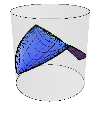
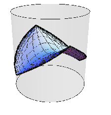
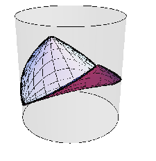
Due to the $\theta$ independence, the tetragon formed by these segments is the same as the boundary of the four cusp solution in [1]. The surfaces (2.17) for different values of the parameter $\theta$ are presented in fig. 3. One can observe that the surfaces have different shapes (extrinsic curvature), but the same boundary.

Thus, we conclude that the boundary of the surfaces (2.17) is $\theta$ -independent, though the shape of surfaces inside the $AdS_{3}$ depends on the parameter $\theta$ .

2.2 The $S^{3}$ projection

Similarly to the $AdS_{3}$ case, we introduce a basis in $\mathbb{R}^{4}$ ( $X$ , $\partial X$ , $\bar{\partial}X,$ $M$ ) with

M\cdot M=1~,~~~~~~X\cdot M=0=\partial X\cdot M=\bar{\partial}X\cdot M~,

(2.24)

and find the linear system formed by the equations

$\displaystyle\partial^{2}X$	$\displaystyle=-X+\frac{\partial\beta}{\sinh\beta}(\cosh\beta\,\partial X-\bar{\partial}X)+vM~,$	(2.25)
$\displaystyle\partial\bar{\partial}X$	$\displaystyle=-\cosh\beta\,X~,$
$\displaystyle\partial M$	$\displaystyle=\frac{v}{\sinh^{2}\beta}(\partial X-\cosh\beta\,\bar{\partial}X)~,$

and their complex conjugated ones. Here

v=\partial^{2}X\cdot M,\qquad\bar{v}=\bar{\partial}^{2}X\cdot M

(2.26)

are the non-zero components of the second fundamental form. The consistency conditions for this linear system lead to the equations

	$\displaystyle\partial\bar{\partial}\beta$	$\displaystyle=-\sinh\beta+\frac{v\bar{v}}{\sinh\beta}~,$		(2.27)
	$\displaystyle\bar{\partial}v$	$\displaystyle=\frac{\partial\beta}{\sinh\beta}\bar{v}~,\qquad\partial\bar{v}=\frac{\bar{\partial}\beta}{\sinh\beta}v~,$		(2.27)

which similarly to the $AdS_{3}$ case admit the constant solution

v=v_{0}~,~~~~~~~\sinh^{2}\beta=|v_{0}|^{2}~.

(2.28)

In the $(\sigma,\tau)$ coordinates the corresponding induced metric $h_{ab}=\partial_{a}X\cdot\partial_{b}X$ and the second fundamental form $V_{ab}=\partial_{a}\partial_{b}X\cdot M$ are

h_{ab}=\left(\begin{array}[]{cc}1+\rho^{2}_{s}&0\\ 0&\rho^{2}_{s}\\ \end{array}\right),\quad V_{ab}=\rho_{s}\sqrt{1+\rho_{s}^{2}}\left(\begin{array}[]{cc}\sin 2\phi_{s}&~~\cos 2\phi_{s}\\ \cos 2\phi_{s}&-\sin 2\phi_{s}\\ \end{array}\right),

(2.29)

where $\rho_{s}$ and $\phi_{s}$ parametrize the solution (2.28)

v_{0}=\frac{2}{i}\,\rho_{s}\sqrt{1+\rho_{s}^{2}}\,\,e^{2i\phi_{s}},

(2.30)

similarly to (2.14).

The mean curvature of the surface in $S^{3}$ is then given by

H_{s}=\frac{1}{2}(h^{-1})_{ab}V_{ba}=-\frac{\sin 2\phi_{s}}{2\rho_{s}\sqrt{1+\rho_{s}^{2}}}~,

(2.31)

and the scalar curvature $R_{s}$ is again zero.

The integration procedure presented in appendix B leads to the following surface in $S^{3}$

X=(\sin\theta_{s}\,\cos\eta_{s},~\cos\theta_{s}\,\cos\xi_{s},~\cos\theta_{s}\,\sin\xi_{s},~\sin\theta_{s}\,\sin\eta_{s})~.

(2.32)

Here $\theta_{s}$ parametrizes the mean curvature as in (2.18)

\cot 2\theta_{s}=H_{s},~~~~~~~~~~~~~~~0<\theta_{s}<\frac{\pi}{2}~.

(2.33)

The worldsheet coordinates $\eta_{s},\,\xi_{s}$ are obtained by the linear transformation

\xi_{s}=A_{s}\,\sigma+B_{s}\,\tau,\qquad\eta_{s}=C_{s}\,\sigma+D_{s}\,\tau~,

(2.34)

with³³ 3 Note that the functional dependence of the coefficients (2.34) on $\rho_{s}$ and $\theta_{s}$ is different from that of the analog coefficients for the AdS part on $\rho$ and $\theta$ .

	$\displaystyle A_{s}$	$\displaystyle=\frac{\sqrt{1+\rho_{s}^{2}}}{\cos\theta_{s}}\,\sqrt{(1+\rho_{s}^{2})\cos^{2}\theta_{s}-\rho_{s}^{2}\,\sin^{2}\theta_{s}}~,$	$\displaystyle B_{s}$	$\displaystyle=\frac{\rho_{s}}{\cos\theta_{s}}\,\sqrt{(1+\rho_{s}^{2})\sin^{2}\theta_{s}-\rho_{s}^{2}\,\cos^{2}\theta_{s}}~,$		(2.35)
	$\displaystyle C_{s}$	$\displaystyle=-\frac{\sqrt{1+\rho_{s}^{2}}}{\sin\theta_{s}}\sqrt{(1+\rho_{s}^{2})\sin^{2}\theta_{s}-\rho_{s}^{2}\,\cos^{2}\theta_{s}}~,$	$\displaystyle D_{s}$	$\displaystyle=\frac{\rho_{s}}{\sin\theta_{s}}\,\sqrt{(1+\rho_{s}^{2})\cos^{2}\theta_{s}-\rho_{s}^{2}\,\sin^{2}\theta_{s}}~.$		(2.35)

Similarly to the $AdS_{3}$ case, we have the freedom in choice of signs of the coefficients $A_{s},B_{s},C_{s},D_{s}$ . The parameters $(\rho_{s},\theta_{s})$ are bounded as in (2.21), which makes (2.35) well defined.

The surface (2.32) corresponds to a torus, where $\theta_{s}$ parametrizes the two radii of the cycles. Using the stereographic projection of $S^{3}$ onto $\mathbb{R}^{3}$ , we present the surfaces (2.32) in fig. 4. The special case $\theta_{s}=0$ or $\theta_{s}=\pi/2$ and $\theta=\pi/4$ is related to the solution in [18].

The induced metric tensor in $AdS_{3}\times S^{3}$ , given as a sum of AdS (2.15) and spherical (2.29) parts, has the form

g_{ab}=f_{ab}+h_{ab}=(1+\rho^{2}+\rho_{s}^{2})\left(\begin{array}[]{cc}1&0\\ 0&1\\ \end{array}\right)~,

(2.36)

and it is conformal due to our construction. We use this metric in section 4 to calculate the worldsheet area.

A last comment concerns the geometric (coordinate invariant) meaning of the four parameters $\theta,\theta_{s},\rho,\rho_{s}$ . As stated in (2.18) and (2.33), $\theta$ and $\theta_{s}$ parametrize the mean curvatures of the projections on $AdS_{3}$ and on $S^{3}$ , whereas $\rho$ and $\rho_{s}$ parametrize the two invariant quantities $(h^{-1})_{ab}~f_{ba}$ and $(f^{-1})_{ab}~h_{ba}$ . Thus, they control the relative size of lengths on the surface measured with respect to $AdS_{3}$ or $S^{3}$ .

3 Embedding in $AdS_{5}$

We now consider an embedding of the surface (2.17) in $AdS_{5}$ . The aim is to realize this in such a manner, that the boundary of the surface is inside the boundary of a single Poincaré patch. To match the generic configuration of the tetragon boundary, we perform boosts, similarly to [1]. However, one has to note that our initial configuration (2.17) is a rotated version of the surface used in [1]. Due to this modification, the relation of the boost parameters to the Mandelstam variables will be different.

$AdS_{5}$ is realized as a hyperboloid in $\mathbb{R}^{2,4}$ with the coordinates $Y\equiv(Y_{0^{\prime}},Y_{0},Y_{1},Y_{2},Y_{3},Y_{4})$ . We first perform a boost in the $(Y_{0},Y_{4})$ plane with a parameter $b>0$

Y_{0}\mapsto\sqrt{1+b^{2}}\,Y_{0}+b\,Y_{4}~,~~~~~~~~~~Y_{4}\mapsto b\,Y_{0}+\sqrt{1+b^{2}}\,Y_{4}~,

(3.1)

and then a boost in the $(Y_{0^{\prime}},Y_{4})$ plane, which we write in the lightcone form

\displaystyle Y_{0^{\prime}}+Y_{4}\mapsto\frac{1}{a}\,\left(Y_{0^{\prime}}+Y_{4}\right)~,~~~~~~~~~~Y_{0^{\prime}}-Y_{4}\mapsto a\left(Y_{0^{\prime}}-Y_{4}\right)~,~~~~~~(a>0).

(3.2)

As a result, from (2.17) we obtain the following surface in $AdS_{5}$

Y_{0}=\sqrt{1+b^{2}}\,\cos\theta\,\cosh\xi~,~~~~Y_{1}=\cos\theta\sinh\xi~,~~~~Y_{2}=\sin\theta\sinh\eta~,~~~~Y_{3}=0~,

(3.3)

Y_{0^{\prime}}+Y_{4}=\frac{1}{a}\,(\sin\theta\,\cosh\eta+b\,\cos\theta\,\cosh\xi)~,~~Y_{0^{\prime}}-Y_{4}=a(\sin\theta\,\cosh\eta-b\,\cos\theta\,\cosh\xi)~.

Introducing the Poincaré coordinates $(r,\,y_{\mu}),$ $(\mu=0,\,1,\,2,\,3)$ , defined as

\displaystyle Y_{\mu}=\frac{y_{\mu}}{r},~~~~~~Y_{0^{\prime}}+Y_{4}=\frac{1}{r}~,~~~~~Y_{0^{\prime}}-Y_{4}=\frac{r^{2}+y_{\mu}y^{\mu}}{r}~,

(3.4)

we find $y_{3}=0$ (we neglect this coordinate below) and

	$\displaystyle r$	$\displaystyle=\frac{a}{\sin\theta\,\cosh\eta+b\,\cos\theta\cosh\xi}~,$	$\displaystyle y_{0}$	$\displaystyle=\frac{a\sqrt{1+b^{2}}\,\cos\theta\,\cosh\xi}{\sin\theta\,\cosh\eta+b\,\cos\theta\cosh\xi}~,$		(3.5)
	$\displaystyle y_{1}$	$\displaystyle=\frac{a\,\cos\theta\,\sinh\xi}{\sin\theta\,\cosh\eta+b\,\cos\theta\cosh\xi}~,$	$\displaystyle y_{2}$	$\displaystyle=\frac{a\,\sin\theta\,\sinh\eta}{\sin\theta\,\cosh\eta+b\,\cos\theta\cosh\xi}~.$		(3.5)

From the analysis of the previous section follows that the edges at the boundary are obtained in the limit $|\xi|\rightarrow\infty$ and $|\eta|\rightarrow\infty$ , with finite $|\xi|-|\eta|.$ Depending on the signs of $\xi$ and $\eta$ there are four possibilities, which correspond to four edges. Obviously, $r\rightarrow 0$ in all these cases.

Let us consider the case $\xi>0$ , $\eta>0$ . Introducing the parameter $\kappa=\xi-\eta$ , in the limit $\xi\rightarrow\infty$ , $\eta\rightarrow\infty$ we obtain

y_{0}=\frac{a\sqrt{1+b^{2}}\cos\theta\,e^{\kappa}}{\sin\theta+b\cos\theta\,e^{\kappa}}~,~~~~~~y_{1}=\frac{a\cos\theta\,e^{\kappa}}{\sin\theta+b\cos\theta\,e^{\kappa}}~,\qquad y_{2}=\frac{a\sin\theta}{\sin\theta+b\,\cos\theta\,e^{\kappa}}~.

(3.6)

These equations define a light-like segment with a $\theta$ -independent relations

y_{0}=\sqrt{1+b^{2}}\,y_{1}~,~~~~~~~b\,y_{1}+y_{2}=a~,

(3.7)

and the coordinate $y_{1}$ is bounded by $0<y_{1}<{a/b}$ . Note that the $\theta$ dependence in (3.6) can also be excluded by the redefinition of the parameter $e^{\kappa}\mapsto\tan\theta\,e^{\kappa}$ . This fact confirms the $\theta$ -independence of the boundary, mentioned in the previous section.

Similarly one can take other limits $\xi\rightarrow\infty$ , $~\eta\rightarrow-\infty$ , $~\xi+\eta=\kappa$ , etc.

The corresponding segments form the tetragon given in fig. 5. The projection of the tetragon on the $(y_{1},\,y_{2})$ plane is the rhombus plotted in fig. 6. Its cusps are located on the axes $y_{1}$ and $y_{2}$ , and the diagonals are equal to ${2a/b}$ and $2a$ , respectively.

The momenta associated with the edges of the tetragon are defined by $2\pi\,k=\Delta y$ , where $\Delta y$ are the shifts of the $y$ coordinates along the segments. In this way the four edges define the following four momenta as in fig. 5

	$\displaystyle k_{1}$	$\displaystyle=\frac{1}{2}\left(\sqrt{-s-t},\,\sqrt{-t},\,-\sqrt{-s}\right),$	$\displaystyle k_{2}$	$\displaystyle=\frac{1}{2}\left(-\sqrt{-s-t},\,-\sqrt{-t},\,-\sqrt{-s}\right),$		(3.8)
	$\displaystyle k_{3}$	$\displaystyle=\frac{1}{2}\left(\sqrt{-s-t},\,-\sqrt{-t},\,\sqrt{-s}\right),$	$\displaystyle k_{4}$	$\displaystyle=\frac{1}{2}\left(-\sqrt{-s-t},\,\sqrt{-t},\,\sqrt{-s}\right)~.$		(3.8)

Here $s$ and $t$ are the Mandelstam variables which are related to the parameters $a,b$ by

-s=2k_{1}\cdot k_{2}=\frac{a^{2}}{\pi^{2}}~,~~~~~~-t=2k_{1}\cdot k_{4}=\frac{a^{2}}{\pi^{2}\,b^{2}}~.

(3.9)

4 Regularized action

Here, we calculate the regularized action for the string solutions given by (2.17) and (2.32). We use the scheme proposed in [2] and take the worldsheet integration over the domain $r(\xi,\eta)>r_{c}$ , where the function $r(\xi,\eta)$ is given by (3.5) and $r_{c}$ is a small parameter. According to (3.5) and (3.9), such a domain is bounded by the contour given as

\epsilon\cosh\eta+\epsilon^{\prime}\cosh\xi=1~,

(4.1)

where

\epsilon=\frac{r_{c}\,\sin\theta}{\pi\sqrt{-s}}~,~~~~~~~\epsilon^{\prime}=\frac{r_{c}\,\cos\theta}{\pi\sqrt{-t}}~.

(4.2)

Fig. 7 shows the curve (4.1) on the $(\xi,\,\eta)$ plane.⁴⁴ 4 Note that in the limit $r_{c}\rightarrow 0$ the edges of the approximate square in fig. 7 correspond to the cusps of the Minkowski space tetragon while the corners are related to the edges of the tetragon.

With the induced metric tensor (2.36) we get for the regularized action

S_{reg}=\frac{\sqrt{\lambda}}{2\pi}(1+\rho^{2}+\rho_{s}^{2})\int_{r>r_{c}}\mbox{d}\sigma\,\mbox{d}\tau~.

(4.3)

The integral term in (4.3) is easier to analyze in the $(\xi,\,\eta)$ coordinates, since the contour which bounds the domain of integration is symmetric there (see fig. 7). The Jacobian of the transformation to $\xi,~\eta$ coordinates defined by (2.20) provides

S_{reg}=\frac{\sqrt{\lambda}}{2\pi}\,\frac{(1+\rho^{2}+\rho_{s}^{2})\sin 2\theta}{\rho\sqrt{1+\rho^{2}}}\,I(r_{c})~,

(4.4)

where

I(r_{c})=\frac{1}{2}\,\int_{r>r_{c}}\mbox{d}\xi\,\mbox{d}\eta~.

(4.5)

This integral is analyzed in appendix C. Up to terms vanishing at $r_{c}\rightarrow 0$ one finds

I(r_{c})=\frac{1}{4}\left(\log\frac{r_{c}^{2}\sin^{2}\theta}{-4\pi^{2}s}\right)^{2}+\frac{1}{4}\left(\log\frac{r_{c}^{2}\cos^{2}\theta}{-4\pi^{2}t}\right)^{2}-\frac{1}{4}\left(\log\frac{s\cot^{2}\theta}{t}\right)^{2}-\frac{\pi^{2}}{3}~.

(4.6)

For $\theta=\pi/4$ this result is in agreement with the corresponding formula in [2].

The expression (4.6) can also be written in the form

I(r_{c})=\frac{1}{4}\left(\log\frac{r_{c}^{2}\cos^{2}\theta}{-4\pi^{2}s}\right)^{2}+\frac{1}{4}\left(\log\frac{r_{c}^{2}\sin^{2}\theta}{-4\pi^{2}t}\right)^{2}-\frac{1}{4}\left(\log\frac{s}{t}\right)^{2}-\frac{1}{4}\left(\log\cot^{2}\theta\right)^{2}-\frac{\pi^{2}}{3}~,

(4.7)

which has the same finite $(s,\,t)$ -dependent part as the BDS formula [20]. This means that for generic $\theta$ , $S_{\rm reg}$ in (4.4), up to the $\theta,\rho,\rho_{s}$ dependent prefactor, is given by the result of [2], with a suitable position dependent cutoff.

In order to match with the BDS formula and the strong coupling behavior of the cusp anomalous dimension, the prefactor in (4.4)

\frac{(1+\rho^{2}+\rho_{s}^{2})\sin 2\theta}{\rho\sqrt{1+\rho^{2}}}

(4.8)

has to be equal to 1. Due to the inequalities (2.21), the minimal value of $\sin 2\theta$ for a given $\rho$ is achieved at the maximal or minimal values of $\tan 2\theta$ (see fig. 1) and one gets

\mbox{min}(\sin 2\theta)=\frac{2\rho\sqrt{1+\rho^{2}}}{1+2\rho^{2}}~.

(4.9)

Hence, the minimal value of the prefactor (4.8) is always greater than 1 and, therefore, there is no finite choice of the parameters $\rho$ , $\rho_{s}$ and $\theta$ to match with the BDS formula. One has to note also that the divergent terms in (4.7) have an asymmetric structure if $\theta\neq\pi/4$ .

5 Conserved charges

5.1 String conserved currents and gluon momenta

The momenta (3.8) can be related to the contour integrations of the conserved currents associated with translations of the Poincaré coordinates in $AdS_{5}$ .

The translations in the Poincaré patch $y^{\mu}\mapsto y^{\mu}+\epsilon^{\mu}$ correspond to the isometry transformations in $AdS_{5}$ , which have the following infinitesimal form

Y^{\mu}\mapsto Y^{\mu}+\epsilon^{\mu}\,Y_{+}~,~~~~~Y_{+}\mapsto Y_{+}~,~~~~~Y_{-}\mapsto Y_{-}+2\epsilon^{\nu}\,Y_{\nu}~,

(5.1)

with $Y_{\pm}=Y_{0^{\prime}}\pm Y_{4}$ . The corresponding Noether currents given by

J^{\mu}_{a}=Y_{+}\,\partial_{a}Y^{\mu}-Y^{\mu}\,\partial_{a}Y_{+}~,

(5.2)

define the 1-forms

J^{\mu}=J_{a}^{\mu}\,d\xi^{a}=Y_{+}\,dY^{\mu}-Y^{\mu}\,dY_{+}~.

(5.3)

In terms of the Poincaré coordinates (3.4), these currents become

J^{\mu}=\frac{dy^{\mu}}{r^{2}}~.

(5.4)

Their integration over a contour with constant $r$ is trivially performed and gives the displacement of $y^{\mu}$ along the contour. Such a contour with $r=r_{c}$ on the worldsheet (3.3) is given by (4.1).

Let us introduce the $r_{c}$ -dependent charge-like object

Q_{1}^{\mu}(r_{c})=\frac{r^{2}_{c}}{2\pi}~\int_{C_{1}}J^{\mu}~,

(5.5)

where the integration contour $C_{1}$ corresponds to the curve (4.1) in the first quarter of the $(\xi,\,\eta)$ plane (see fig. 7). From (5.4) follows $Q_{1}^{\mu}(r_{c})=y^{\mu}(\xi_{c},0)-y^{\mu}(0,\eta_{c})$ . The function $y^{\mu}(\xi,\eta)$ here is given by (3.5) and its arguments $(\xi_{c},0)$ and $(0,\eta_{c})$ are the points where the contour (4.1) intersects the axes $\xi$ and $\eta$ , respectively. Recalling then the definition of the $k_{1}$ vector in (3.8) we find

\lim_{r_{c}\rightarrow 0}Q_{1}^{\mu}(r_{c})=k_{1}^{\mu}~.

(5.6)

The other momenta in (3.8) are obtained by the shifts of the contour $C_{1}$ to the corresponding quarters in the $(\xi,\,\eta)$ plane.

5.2 Charges at the cusps

Now we would like to study some charges carried by the string, which can be associated to the cusps of the tetragon. As explicit examples we consider the charges related to the translation currents for the $AdS_{5}$ part (5.2) and those related to the rotations in the $(X_{1},X_{4})$ and the $(X_{2},X_{3})$ planes for the $S^{3}$ part.

For the solution (3.3) the translation currents (5.2) take the form

$\displaystyle J^{0}_{\xi}$	$\displaystyle=-\frac{\sqrt{1+b^{2}}}{2a}\,\sin 2\theta\,\sinh\xi\,\cosh\eta~,$	$\displaystyle J^{0}_{\eta}$	$\displaystyle=\frac{\sqrt{1+b^{2}}}{2a}\,\sin 2\theta\,\cosh\xi\,\sinh\eta~,$	(5.7)
$\displaystyle J^{1}_{\xi}$	$\displaystyle=\frac{1}{2a}\,\sin 2\theta\,\cosh\xi\,\cosh\eta+\frac{b}{a}\,\cos^{2}\theta~,$	$\displaystyle J^{1}_{\eta}$	$\displaystyle=-\frac{1}{2a}\,\sin 2\theta\,\sinh\xi\,\sinh\eta~,$
$\displaystyle J^{2}_{\xi}$	$\displaystyle=-\frac{b}{2a}\,\sin 2\theta\,\sinh\xi\,\sinh\eta~,$	$\displaystyle J^{2}_{\eta}$	$\displaystyle=\frac{b}{2a}\,\sin 2\theta\,\cosh\xi\,\cosh\eta+\frac{1}{a}\,\sin^{2}\theta~.$

Here the upper index $\mu$ refers to the embedding space $(\mu=0,1,2)$ , and the lower index to the worldsheet.

The rotational currents for the $S^{3}$ projection (2.32) have their simplest form in the $(\xi_{s},\,\eta_{s})$ coordinates

J^{14}_{\xi_{s}}=0~,\quad J^{14}_{\eta_{s}}=\sin\theta_{s}~;\quad\quad J^{23}_{\xi_{s}}=\cos\theta_{s}~,\quad J^{23}_{\eta_{s}}=0~.

(5.8)

The worldsheet boundary analysis is most natural in $(\xi,\,\eta)$ coordinates. To simplify the discussion, we therefore restrict ourselves to the special case where $(\xi_{s},\,\eta_{s})$ and $(\xi,\,\eta)$ have a diagonal transformation matrix. Then the parameters in (2.19) and (2.34) have to satisfy

\frac{A}{B}=\frac{A_{s}}{B_{s}}\,,\qquad\frac{C}{D}=\frac{C_{s}}{D_{s}}\,.

(5.9)

These conditions are fulfilled for $B=B_{s}=C=C_{s}=0$ ,⁵⁵ 5 Besides the reversed situation with minimal value of $\theta$ for a fixed $\rho$ etc, there are no other solutions. which give the maximal value of $\theta$ for a fixed $\rho$ , where $\tan 2\theta=-2\rho\sqrt{1+\rho^{2}}$ (see fig. 1) and minimal value of $\theta_{s}$ for a fixed $\rho_{s}$ , where $\tan 2\theta_{s}=2\rho_{s}\sqrt{1+\rho_{s}^{2}}$ . This leads to the following relations between the worldsheet coordinates

\xi=\frac{\sigma}{\sqrt{-\cos 2\theta}}=\sqrt{-\frac{\cos 2\theta_{s}}{\cos 2\theta}}\,\,\xi_{s}~,\quad\eta=\frac{\tau}{\sqrt{-\cos 2\theta}}=\sqrt{-\frac{\cos 2\theta_{s}}{\cos 2\theta}}\,\,\eta_{s}~.

(5.10)

The $(\xi,\,\eta)$ -components of the currents (5.8) then read

J^{14}_{\xi}=0~,\quad J^{14}_{\eta}=\sqrt{-\frac{\cos 2\theta}{\cos 2\theta_{s}}}\,\,\sin\theta_{s}~;~~~\quad J^{23}_{\xi}=\sqrt{-\frac{\cos 2\theta}{\cos 2\theta_{s}}}\,\,\cos\theta_{s}~,\quad J^{23}_{\eta}=0~.

(5.11)

Furthermore, for these special extremal correlations between $\theta$ and $\rho$ as well as between $\theta_{s}$ and $\rho_{s}$ , the prefactor in the action (4.8) can be written as

\frac{(1+\rho^{2}+\rho_{s}^{2})\sin 2\theta}{\rho\sqrt{1+\rho^{2}}}=1-\frac{\cos 2\theta}{\cos 2\theta_{s}}~,

(5.12)

which has a simple form in terms of the charges we will find below in (5.20). For $\theta\sim{\pi/4}$ and generic $\theta_{s}$ this is a small deformation away from unity, which is the strong coupling limit of the universal scaling function, or cusp anomalous dimension. One may hope that it could be related to some generalization of the cusp anomalous dimension similar to that discussed in [21, 18].

To get an overview of the sources and sinks of the fluxes related to the worldsheet vector fields (5.7) and (5.11), we analyze the corresponding flux lines.

For the rotational currents these are trivially identified as straight lines parallel to the $\eta$ -axis or parallel to the $\xi$ -axis for $J^{14}$ or for $J^{23}$ , respectively. This means in both cases that all flux originates from one cusp of the tetragon and flows to the corresponding opposite cusp. There are no other sources or sinks of flux, neither at other points of the boundary nor in the interior of the tetragon surface.

The fluxes of the translational currents require a little bit more effort. The flux lines for $J^{0}$ from (5.7) are given by

\sinh\xi~\sinh\eta~=~c~.

(5.13)

The set of flux lines is parametrized by $-\infty<c<\infty$ . For the two other currents we restrict to large $\xi$ and/or $\eta$ . Then in (5.7) the constant terms can be neglected and the integration becomes simple again. For $J^{1}$ and $J^{2}$ the flux lines are given by

\cosh\xi~\sinh\eta~=~c~~~\mbox{and}~~~\cosh\eta~\sinh\xi~=~c~,

(5.14)

respectively. These fluxes are most efficiently visualized in the plane spanned by the variables $x=\sinh\xi$ and $y=\sinh\eta$ , see fig. 8. There the flux lines of $J^{0}$ are hyperbolas. The flux lines of $J^{1}$ behave for large $x$ like hyperbolas, but cross the $y$ -axis at finite values. For $J^{2}$ the role of $x$ and $y$ in this picture is interchanged.

From this analysis we see that also the fluxes of the translation currents have their sources and sinks at the cusps, exclusively. Following standard terminology, we call these sources and sinks charges. Then the current $J^{0}$ has charges at all four cusps. The sign of the charges alternates, if one goes around the tetragon. The two other currents have zero charge at two opposite cusps and charges of different sign at the respective other pair of opposite cusps.

Obviously, the charges are divergent and need some regularization. Of course, as usual, regularization is ambigous. However, after treating the area problem via a regularized boundary according to (4.1), it is natural to generate the regularization of the charges also via this regularized boundary. Therefore, we divide the regularized boundary into charged and uncharged segments. A negatively charged segment is understood as a connected piece of the regularized boundary, on which all flux lines cross from inside and flow to the same cusp. A positively charged segment is a connected piece of the regularized boundary, on which all flux lines cross from outside and originate from the same cusp. An uncharged segment is a connected piece of the regularized boundary, on which all crossing flux lines come back at another crossing point.

As the regularization of the charge sitting at a cusp we define the flux through the charged segment of the regularized boundary, to which the cusp is connected via its flux lines. For the flows under discussion this division in segments is exhaustive and a cusp is connected via its flux lines at most to one charged segment. If it is not connected to a charged segment, its charge is zero.

The flux through a contour $C$ is given by

F_{C}=\int_{C}\mbox{d}\xi^{a}\,\epsilon_{ab}\,\sqrt{g}\,\,g^{bc}\,J_{c}~=~\int_{C}\mbox{d}\xi\,\,J_{\eta}-\mbox{d}\eta\,J_{\xi}~.

(5.15)

Note that the rightmost representation is valid since for the subclass of surfaces under consideration, due to (5.10), $\xi$ and $\eta$ are conformal coordinates.

Now we have to identify the points on the regularized boundary, which define the division into segments. In the $(x,y)$ plane the regularized boundary (4.1), (4.2) is given by

\epsilon~\sqrt{1+y^{2}}~+~\epsilon^{\prime}~\sqrt{1+x^{2}}~=~1~.

(5.16)

Asymptotically, for $r_{c}\rightarrow 0$ , this is a rhombus with corners at the axes at $\pm 1/\epsilon^{\prime}$ and $\pm 1/\epsilon$ , respectively ⁶⁶ 6 In contrast to the picture in the $(\xi,\eta)$ plane, the corners now correspond to the cusps of the AdS tetragon surface.. It is shown together with the fluxes for $J^{0}$ and $J^{1}$ in fig. 8.

For $J^{0}$ one gets four charged segments. The points defining the division are determined by the condition, that there the corresponding edge of the rhombus is tangential to one of the flux line hyperbolas $x~y=c$ . The coordinates of these four points turn out as $(\pm\frac{1}{2\epsilon^{\prime}},\pm\frac{1}{2\epsilon})$ (up to terms staying finite for $r_{c}\rightarrow 0$ ).

Let us enumerate the cusps in clockwise manner, starting with that related to the positive $y$ -axis. Then $F_{1}^{0}$ , the regularized charge for $J^{0}$ at cusp 1, is given by (5.15), where the contour $C$ is the piece of the regularized boundary in the $(\xi,\eta)$ plane between the points $(\mbox{arcsinh}\ \frac{1}{2\epsilon^{\prime}},\mbox{arcsinh}\ \frac{1}{2\epsilon})$ and $(-\mbox{arcsinh}\ \frac{1}{2\epsilon^{\prime}},\mbox{arcsinh}\ \frac{1}{2\epsilon})$ . Due to flux conservation the integration contour can be replaced by the straight line connecting these two points. Then using (5.7), (3.9) and (4.2) we get

F^{0}_{1}~=~\sqrt{-s-t}~\frac{\pi}{2r_{c}^{2}}~+~O(1)~.

(5.17)

Now we define rescaled (renormalized) translation charges via (compare to (5.5))

q^{\mu}_{a}=\lim_{r_{c}\rightarrow 0}\frac{r_{c}^{2}}{2\pi}~F^{\mu}_{a}

(5.18)

and get after repeating the calculation for the other cusps and the currents $J^{1}$ and $J^{2}$

$\displaystyle q^{0}_{1}$	$\displaystyle=\frac{1}{4}\ \sqrt{-s-t}~,$	$\displaystyle q^{1}_{1}$	$\displaystyle=0~,$	$\displaystyle q^{2}_{1}$	$\displaystyle=\frac{1}{4}\ \sqrt{-s}~,$	(5.19)
$\displaystyle q^{0}_{2}$	$\displaystyle=-\frac{1}{4}\ \sqrt{-s-t}~,$	$\displaystyle q^{1}_{2}$	$\displaystyle=\frac{1}{4}\ \sqrt{-t}~,$	$\displaystyle q^{2}_{2}$	$\displaystyle=0~,$
$\displaystyle q^{0}_{3}$	$\displaystyle=\frac{1}{4}\ \sqrt{-s-t}~,$	$\displaystyle q^{1}_{3}$	$\displaystyle=0~,$	$\displaystyle q^{2}_{3}$	$\displaystyle=-\frac{1}{4}\ \sqrt{-s}~,$
$\displaystyle q^{0}_{4}$	$\displaystyle=-\frac{1}{4}\ \sqrt{-s-t}~,$	$\displaystyle q^{1}_{4}$	$\displaystyle=-\frac{1}{4}\ \sqrt{-t}~,$	$\displaystyle q^{2}_{4}$	$\displaystyle=0~.$

For the rotation currents the regularized boundary has only two charged segments, each segment consists out of two adjacent edges of the rhombus. The currents are constant, giving regularized charges proportional to the length of the integration contours in the $(\xi,\eta)$ plane, i.e. proportional to $\log r_{c}$ . If one would apply the same rescaling recipe as for the translation currents, one would get zero renormalized charges for all cusps. We prefer to apply a rescaling, which just cancels the logarithmic divergence and get

$\displaystyle q^{14}_{1}$	$\displaystyle=\sqrt{-\frac{\cos 2\theta}{\cos 2\theta_{s}}}~\sin\theta_{s}~,$	$\displaystyle q^{23}_{1}$	$\displaystyle=0~,$	(5.20)
$\displaystyle q^{14}_{2}$	$\displaystyle=0~,$	$\displaystyle q^{23}_{2}$	$\displaystyle=\sqrt{-\frac{\cos 2\theta}{\cos 2\theta_{s}}}~\cos\theta_{s}~,~~~~~~$
$\displaystyle q^{14}_{3}$	$\displaystyle=-\sqrt{-\frac{\cos 2\theta}{\cos 2\theta_{s}}}~\sin\theta_{s}~,$	$\displaystyle q^{23}_{3}$	$\displaystyle=0~,$
$\displaystyle q^{14}_{4}$	$\displaystyle=0~,$	$\displaystyle q^{23}_{4}$	$\displaystyle=-\sqrt{-\frac{\cos 2\theta}{\cos 2\theta_{s}}}~\cos\theta_{s}~.$

Note that $q^{1}$ and $q^{2}$ are parallel to $q^{23}$ and $q^{14}$ from (5.20) as four-vectors.

Another interesting point is the relation between the charges (5.19) and the gluon momenta (3.8) that can be written in contravariant coordinates as

k_{n}^{0}~=~q_{n+1}^{0}-q_{n}^{0}~,\quad\quad k_{n}^{i}~=~2\ (q_{n+1}^{i}-q_{n}^{i})~,\quad(i=1,2)~,\quad(n=1,...,4)~~(q_{5}=q_{1})~,

(5.21)

which is quite similar to the result of the previous subsection.

6 Analytic continuation of the $AdS_{3}$ projection

Here we describe how to get a new space-like string solution in $AdS_{3}\times S^{3}$ with a time-like $AdS_{3}$ projection from (2.17).

Let us continue analytically the two parameters $\rho\mapsto-i\rho$ and $\theta\mapsto i\theta$ that the $AdS_{3}$ projection (2.17) depends on. This procedure leaves the worldsheet coordinates $\xi$ and $\eta$ real, but makes the components $\,Y_{0^{\prime}}\,$ and $\,Y_{2}\,$ pure imaginary and thus they effectively exchange positions. Then, the new solution of the system (2.3) is

Y_{0^{\prime}}=\sinh\theta\,\sinh\eta,\quad Y_{0}=\cosh\theta\,\cosh\xi,\quad Y_{1}=\cosh\theta\,\sinh\xi,\quad Y_{2}=\sinh\theta\,\cosh\eta,

(6.1)

where

\xi=A\,\sigma+B\,\tau,\qquad\eta=C\,\sigma+D\,\tau,

(6.2)

with

	$\displaystyle A$	$\displaystyle=\frac{\rho}{\cosh\theta}\,\sqrt{(1-\rho^{2})\sinh^{2}\theta-\rho^{2}\,\cosh^{2}\theta}~,$	$\displaystyle B$	$\displaystyle=\frac{\sqrt{1-\rho^{2}}}{\cosh\theta}\,\sqrt{(1-\rho^{2})\cosh^{2}\theta-\rho^{2}\,\sinh^{2}\theta}~,$		(6.3)
	$\displaystyle C$	$\displaystyle=\frac{\rho}{\sinh\theta}\,\sqrt{(1-\rho^{2})\cosh^{2}\theta-\rho^{2}\,\sinh^{2}\theta}~,$	$\displaystyle D$	$\displaystyle=\frac{\sqrt{1-\rho^{2}}}{\sinh\theta}\sqrt{(1-\rho^{2})\sinh^{2}\theta-\rho^{2}\,\cosh^{2}\theta}~.$		(6.3)

Note that the signs of all coefficients in this equation are now positive. However, there is a freedom to change signs of an even number of the coefficients, like for the solution (2.17).

The parameters $\rho$ and $\theta$ are constrained in such a way that the square roots in (6.3) are real, which means

\rho^{2}\leq\frac{\sinh^{2}\theta}{1+2\sinh^{2}\theta}~.

(6.4)

The induced metric for the $AdS_{3}$ projection is time-like and in the $(\sigma,\tau)$ coordinates it is given by $f_{ab}={\rm diag}(-\rho^{2},1-\rho^{2})$ . The full surface, including the contribution from the sphere (2.32) renders the total induced metric Euclidean and conformal, with conformal factor $1-\rho^{2}+\rho_{s}^{2}$ . The new $AdS_{3}$ projection is visualized in fig. 9 for different values of $\theta$ .

As opposed to the case studied in section 2, here pairs of consecutive edges go forward in time, so one pair of the cusps has a time-like separation.

The solution (6.1) can also be obtained in a systematic way by the Pohlmeyer reduction. One has to use again complex conformal coordinates, which for the time-like $AdS_{3}$ projection yield $-1\leq\partial Y\cdot\bar{\partial}Y\leq 1$ . Then, one can use the parametrization $\partial Y\cdot\bar{\partial}Y=\cos\alpha$ , which modifies the linear equations (2.11) and the consistency conditions (2.12). Note also that the normal vector $N$ is now space-like. Finally, a constant solution of the consistency condition, after exponentiation leads to (6.1).

7 Time-like surfaces in $AdS_{3}\times S^{3}$

The example of the previous section inspires a construction of time-like worldsheets in $AdS_{3}\times S^{3}$ . In this case the conformal worldsheet coordinates $z=\frac{1}{2}(\sigma+\tau)$ and $\bar{z}=\frac{1}{2}(\sigma-\tau)$ are real.

The components of the stress tensor become chiral and they can be turned to a constant

\partial Y\cdot\partial Y=-\mu^{2}=\bar{\partial}Y\cdot\bar{\partial}Y,\quad\partial X\cdot\partial X=\mu^{2}=\bar{\partial}X\cdot\bar{\partial}X~.

(7.1)

Here one has to distinguish infinite open strings and closed strings. In the case of infinite strings the worldsheet is described by a plane and using a rescaling of worldsheet coordinates one can put $\mu=1$ . We present two solutions for infinite strings. Their structure is defined by elements of the $o(2,2)$ algebra that one needs to exponentiate in the integration procedure of the linear system.

The first solution is the hyperbolic case (fig. 10a)

	$\displaystyle Y_{0^{\prime}}$	$\displaystyle=\sinh\theta\,\sinh\eta\,\cos\xi-\cosh\theta\,\cosh\eta\,\sin\xi,$	$\displaystyle Y_{0}$	$\displaystyle=\sinh\theta\,\sinh\eta\,\sin\xi+\cosh\theta\,\cosh\eta\,\cos\xi,$		(7.2)
	$\displaystyle Y_{1}$	$\displaystyle=\sinh\theta\,\cosh\eta\,\sin\xi+\cosh\theta\,\sinh\eta\,\cos\xi,$	$\displaystyle Y_{2}$	$\displaystyle=\sinh\theta\,\cosh\eta\,\cos\xi-\cosh\theta\,\sinh\eta\,\sin\xi~,$		(7.2)

and the second one is the parabolic (fig. 10b)

	$\displaystyle Y_{0^{\prime}}$	$\displaystyle=-\eta\,\cos\xi-\sin\xi,$	$\displaystyle Y_{0}$	$\displaystyle=-\eta\,\sin\xi+\cos\xi,$		(7.3)
	$\displaystyle Y_{1}$	$\displaystyle=\eta\,\cos\xi,$	$\displaystyle Y_{2}$	$\displaystyle=-\eta\,\sin\xi.$		(7.3)

The parameter $\theta$ in (7.2) is again related to the extrinsic curvature and the new worldsheet coordinates $(\xi,\,\eta)$ are given by a linear transformation as in (2.19). The equation of motion and the Virasoro constraints (7.1) provide three conditions for the coefficients $A$ , $B$ , $C$ , $D$ . Taking into account the $\theta$ -dependence, one gets a two parameter family of solutions, as in the space-like case.

The closed string solutions satisfy the periodicity condition $\sigma\sim\sigma+2\pi$ . In this case $\mu$ stands as an additional parameter, but the coefficients $A$ and $C$ become integers. The corresponding worldsheets are defined by the exponentiation of the time-like elements in the $o(2,2)=sl(2)\oplus sl(2)$ decomposition and lead to the elliptic solution (fig. 10c)

Y_{0^{\prime}}=\cosh\theta\,\sin\eta,\quad Y_{0}=\cosh\theta\,\cos\eta,\quad Y_{1}=\sinh\theta\,\sin\xi,\quad Y_{2}=\sinh\theta\,\cos\xi~,

(7.4)

where

\xi=k\,\sigma+\kappa\,\tau,\qquad\eta=l\,\sigma+\lambda\,\tau,

(7.5)

with integers $k$ and $l$ . The equation of motion and the Virasoro constraints now provide three equations

	$\displaystyle(l^{2}+\lambda^{2})\cosh^{2}\theta-(k^{2}+\kappa^{2})\sinh^{2}\theta$	$\displaystyle=\mu^{2}$		(7.6)
	$\displaystyle k^{2}-\kappa^{2}=l^{2}-\lambda^{2},\qquad k\kappa\sinh^{2}\theta$	$\displaystyle=l\lambda\cosh^{2}\theta~,$		(7.6)

and one can use $k$ , $l$ and $\mu$ to parameterize the solutions.

The spherical part of the time-like solutions formally coincides with (2.32). However, the conditions for the coefficients $A_{s}$ , $B_{s}$ , $C_{s}$ , $D_{s}$ now are modified. In the periodic case one has

\xi_{s}=k_{s}\,\sigma+\kappa_{s}\,\tau,\qquad\eta_{s}=l_{s}\,\sigma+\lambda_{s}\,\tau,

(7.7)

with integers $k_{s},\,l_{s}$ and one finds equations similar to (7.6)

	$\displaystyle(k_{s}^{2}+\kappa_{s}^{2})\cos^{2}\theta_{s}+(l_{s}^{2}+\lambda_{s}^{2})\sin^{2}\theta_{s}$	$\displaystyle=\mu^{2}$		(7.8)
	$\displaystyle k_{s}^{2}-\kappa_{s}^{2}=l_{s}^{2}-\lambda_{s}^{2},\qquad k_{s}\kappa_{s}\cos^{2}\theta_{s}$	$\displaystyle=-l_{s}\lambda_{s}\sin^{2}\theta_{s}~.$		(7.8)

Closed string worldsheets constructed in this way generalize string solutions in $AdS_{3}\times S^{1}$ and $R^{1}\times S^{3}$ discussed in [23].

8 Conclusions

We have constructed a four parameter family of string solutions in $AdS_{5}\times S^{5}$ whose boundary approaches the light-like tetragon and are a generalization of the solution of [1]. These minimal surfaces are space-like and flat. Their projections on each of the $AdS_{5}$ and $S^{5}$ have constant mean curvature. As the surface approaches the boundary of $AdS_{5}$ it wraps a torus inside $S^{5}$ an infinite number of times. The solutions therefore satisfy Neumann boundary conditions on $S^{5}$ .

The construction used the Pohlmeyer reduction for $AdS_{3}\times S^{3}$ and is based on a constant solution of the reduced system. After knowing the solution, it is instructive to describe it by a direct ad hoc construction as follows. Up to isometry, the tetragon surface of [1] can be characterized as a part of the intersection of the AdS hyperboloid with the hypersurface $Y_{0}^{2}-Y_{1}^{2}={1/2}$ . The straightforward deformation to $Y_{0}^{2}-Y_{1}^{2}=\cos^{2}\theta$ with the explicit parametrization (2.17) is no longer minimal in $AdS_{3}$ . However, this deformation does not modify the behavior of the hypersurface at infinity, resulting in the same boundary behavior. With the parametrization (2.17) the surface obeys the equation of motion (2.4),(2.6), but not the pure AdS Virasoro constraints. After a suitable linear transformation to new coordinates ( $\sigma$ and $\tau$ in the main text) one can achieve $\partial Y\cdot\partial Y=-1$ . It is therefore necessary to include also a nontrivial projection on $S^{5}$ satisfying $\partial X\cdot\partial X=1$ such that the total Virasoro condition is satisfied $\partial Y\cdot\partial Y+\partial X\cdot\partial X=0$ . The $AdS_{5}$ part and the $S^{5}$ are essentially decoupled, their only correlation is given via the Virasoro constraint [12].

Applying suitable isometry transformations in $AdS_{5}$ , the boundary can fit any null tetragon spanned by four light-like vectors pointing alternating forward and backward in time. Interpreting these vectors as momenta of a four-point scattering amplitude of massless particles in Minkowski space allows us to characterize the tetragon by the Mandelstam variables $s$ and $t$ . The area of our surface, regulated by a constant cutoff in the radial coordinate of an $AdS_{5}$ Poincaré patch has been calculated. Up to a prefactor, depending on the parameters $\theta,~\rho$ and $\rho_{s}$ , it is given by the same expression as the area for the pure $AdS_{5}$ tetragon surface used in the Alday-Maldacena conjecture with a position dependent cutoff [2].⁷⁷ 7 Given that the surface satisfies Neumann boundary conditions on the $S^{5}$ coordinates, the classical action should include an extra Legendre-transformation boundary term. This term is proportional to the circumference of the loop times the relevant momenta and has a logarithmic divergence that is subleading with respect to the bulk $\log^{2}$ divergence. The prefactor is generically larger than one. It approaches the value one only in the limiting case $\theta=\pi/4,~~\rho\rightarrow\infty$ . Then the $AdS_{5}$ projection is just the tetragon surface of [1] and the limit $\rho\rightarrow\infty$ suppresses the weight of the $S^{5}$ projection relative to the $AdS_{5}$ part.

An additional observation was made via the continuation $\theta\rightarrow i\theta$ and $\rho\rightarrow-i\rho$ connected with a Wick rotation for one of the time-like and one of the space-like $\mathbb{R}^{2,4}$ coordinates. The resulting minimal surface is still space-like concerning the metric induced from $AdS_{5}\times S^{5}$ . However, the induced metric of its $AdS_{5}$ projection is time-like. This projection approaches a null tetragon at the boundary. In the original null tetragon the sides were consecutively running up and down in time. Now, after this continuation, these null tetragons contain two cusps with adjacent momenta pointing in the same direction of time. In the language of scattering amplitudes the surface would correspond directly to the physical configuration in the $s$ - or $t$ -channel and not, as before continuation, to that in the $u$ -channel.

One may think that our solutions are subleading contribution to the usual gluon scattering amplitude. However, as we have shown in section 5, these solutions carry extra quantum numbers, which are momenta on the sphere, or $R$ -charge in the gauge theory. These surface therefore describe different Wilson loop observables and if they describe scattering amplitudes, then these are also somewhat different. One would expect the dual Wilson loop to have insertions of the appropriate scalar fields carrying these charges (similar to [22]). In the particular setup analyzed in section 5, the $AdS_{3}$ and $S^{3}$ parts of the solution are chosen to align. In that case the charges are localized at the cusps and each corresponds to rotation in a single plane. Therefore, one would expect the dual Wilson loop to have insertions of the form $Z^{F_{14}}$ , $X^{F_{23}}$ , $\bar{Z}^{F_{14}}$ , $\bar{X}^{F_{23}}$ where $Z$ and $X$ are two complex scalars. In the more general case these insertions could be along the edges.⁸⁸ 8 Alternatively, it may involve insertions at the cusps of appropriate (complicated) operators carrying two angular momenta. It would be interesting to study these insertions on the gauge theory side to see if similar structure arises also in perturbation theory.

The solutions carrying a single charge at each cusp have the additional nice feature that in each of the quadrants in the $(\xi,\,\eta)$ plane both the $AdS_{3}$ and the $S^{3}$ coordinates have a uniform behavior, exponential in the $AdS_{3}$ part and oscillatory in the $S^{3}$ part. In the construction of the solutions for more general light-like polygons [4, 9], such regions on the worldsheet with uniform asymptotics play a crucial role. It is natural to expect that similar generalization would apply to our construction.

It is of course tempting to speculate that such solutions may represent scattering amplitudes other than the MHV ones, which seem to be captured purely by the $AdS$ solutions. Clearly this should not be the case of these specific solutions, since for four gluons all amplitudes are either MHV or they vanish. Still, since some generalization is necessary to describe non-MHV amplitudes for higher-point functions, it is natural to look for solutions similar to the ones presented here which end on more light-like segments on the boundary.

In a final addendum, we indicated how our procedure for space-like string surfaces can be translated to the study of dynamical strings and gave examples for related explicit solutions. Besides a complete description of all solutions in this class, further study should explore how they fit into previously studied cases and in particular into the general classification given in [24].

Acknowledgements

We thank J. Henn, K. Jin, J. Plefka, C. Vergu, S. Wuttke and D. Young for useful discussions. This work has been supported in part by Deutsche Forschungsgemeinschaft via SFB 647. G.J. was also supported by GNSF.

Appendix A Integration of the linear system in $\mathbb{R}^{2,2}$

In this appendix we construct the string surface corresponding to the solution (2.13)-(2.14).

We use covariant notations $(\sigma,\,\tau)$ = $(\xi^{1},\xi^{2})$ ; $\,\partial_{\sigma}=\partial_{1}$ , $\partial_{\tau}=\partial_{2},\,$ and introduce the basis related to these real worldsheet coordinates

e_{0^{\prime}}=N~,~~~~e_{0}=Y~,~~~~e_{1}=\frac{\partial_{1}Y}{\rho}~,~~~~e_{2}=\frac{\partial_{2}Y}{\sqrt{1+\rho^{2}}}~.

(A.1)

From (2.15) follow the orthonormality conditions $e_{m}\cdot e_{n}=\mbox{diag}(-1,-1,1,1).$

For a given $Y$ , $\partial_{1}Y$ and $\partial_{2}Y$ , the normal vector $N$ can be fixed by

e_{0^{\prime}}\,^{n}=\epsilon^{n}\,_{mlk}\,e_{2}\,^{m}e_{1}\,^{l}e_{0}\,^{k}~,

(A.2)

where $\epsilon^{n}\,_{mlk}$ is the Levi-Civita tensor, with $\epsilon_{0^{\prime}012}=1$ , and upper letters correspond to the vector indices of the basis elements. Then, $e_{m}^{~~n}\in SO_{\uparrow}(2,2)$ , i.e.

\mbox{det}\,e_{m}^{~~n}=1~,\quad e_{0^{\prime}}\,^{0^{\prime}}e_{0}\,^{0}-e_{0^{\prime}}\,^{0}e_{0}\,^{0^{\prime}}\geq 1~.

(A.3)

The vector $\partial_{t}Y$ , where $t$ is the global time variable (2.23), defines the time direction. From (A.3) follows $N\cdot\partial_{t}Y\leq-1$ , which indicates that $N$ is oriented to the time direction.

Similarly to (2.11), the basis vectors (A.1) satisfy the linear equations

\partial_{1}e=A_{1}\,e~,~~~~~\qquad\partial_{2}{e}=A_{2}\,e~.

(A.4)

The matrices $A_{1}$ and $A_{2}$ here belong to the $o(2,2)$ algebra and they have the following block structure

A_{1}=\left(\begin{array}[]{cc}0&B_{1}\\ B_{1}^{T}&0\\ \end{array}\right),~~~~~~~~~A_{2}=\left(\begin{array}[]{cc}0&B_{2}\\ B_{2}^{T}&0\\ \end{array}\right),

(A.5)

with $2\times 2$ matrices

B_{1}=\left(\begin{array}[]{cc}\sqrt{1+\rho^{2}}\,\sin 2\phi&\rho\,\cos 2\phi\\[5.69046pt] \rho&0\\ \end{array}\right),~~~~~~B_{2}=\left(\begin{array}[]{cc}\sqrt{1+\rho^{2}}\,\cos 2\phi&-\rho\,\sin 2\phi\\[5.69046pt] 0&\sqrt{1+\rho^{2}}\\ \end{array}\right).

(A.6)

The integrability of the system (A.4) is provided by $[A_{1},\,A_{2}]=0$ and one gets the solution

e=\exp(\xi^{i}A_{i})\,\,C~,

(A.7)

where $C$ is a constant $SO_{\uparrow}(2,2)$ matrix. The worldsheet $Y(\sigma,\,\tau)$ can be read off from the second row of this solution. In the following we explain how to calculate the exponential in (A.7), using the decomposition $SO_{\uparrow}(2,2)=SL(2,R)\times SL(2,R)$ .

The $SL(2,R)$ generators $t_{\alpha}$ $(\alpha=0,1,2)$ given by

t_{0}=\left(\begin{array}[]{cc}0&1\\ -1&0\\ \end{array}\right),\quad t_{1}=\left(\begin{array}[]{cc}0&1\\ 1&0\\ \end{array}\right),\quad t_{2}=\left(\begin{array}[]{cc}1&0\\ 0&-1\\ \end{array}\right),

(A.8)

satisfy the relations

t_{\alpha}t_{\beta}=\eta_{\alpha\beta}\,I+{\epsilon_{\alpha\beta}}^{\gamma}\,t_{\gamma}~,

(A.9)

where $\eta_{\alpha\beta}=\mbox{diag}(-1,1,1)$ is the metric tensor of 3d Minkowski space, $I$ denotes the $2\times 2$ unit matrix and $\epsilon_{\alpha\beta\gamma}$ is the Levi-Civita tensor with $\epsilon_{012}=1$ .

Let us introduce $4\times 4$ matrices

	$\displaystyle L_{0}$	$\displaystyle=\left(\begin{array}[]{cc}t_{0}&0\\ 0&t_{0}\\ \end{array}\right),$	$\displaystyle L_{1}$	$\displaystyle=\left(\begin{array}[]{cc}0&t_{1}\\ t_{1}&0\\ \end{array}\right),$	$\displaystyle L_{2}$	$\displaystyle=\left(\begin{array}[]{cc}0&t_{2}\\ t_{2}&0\\ \end{array}\right),$		(A.10)
	$\displaystyle R_{0}$	$\displaystyle=\left(\begin{array}[]{cc}t_{0}&0\\ 0&-t_{0}\\ \end{array}\right),$	$\displaystyle R_{1}$	$\displaystyle=\left(\begin{array}[]{cc}0&-t_{0}\\ t_{0}&0\\ \end{array}\right),$	$\displaystyle R_{2}$	$\displaystyle=\left(\begin{array}[]{cc}0&I\\ I&0\\ \end{array}\right).$		(A.10)

They form a basis in $o(2,2)$ and satisfy the relations (similar to (A.9))

L_{\alpha}L_{\beta}=\eta_{\alpha\beta}\,\hat{I}+{\epsilon_{\alpha\beta}}^{\gamma}\,L_{\gamma}~,~~~~~~~~R_{\alpha}R_{\beta}=\eta_{\alpha\beta}\,\hat{I}+{\epsilon_{\alpha\beta}}^{\gamma}\,R_{\gamma}~,

(A.11)

where $\hat{I}$ is the $4\times 4$ unit matrix. In addition, the matrices $L_{\alpha}$ commute with $R_{\beta}$ , $\,\left[L_{\alpha},R_{\beta}\right]=0$ . From (A.11) follow the commutation relations of the $sl(2)$ algebra

\left[L_{\alpha},L_{\beta}\right]=2{\epsilon_{\alpha\beta}}^{\gamma}\,L_{\gamma}~,~~~~~\left[R_{\alpha},R_{\beta}\right]=2{\epsilon_{\alpha\beta}}^{\gamma}\,R_{\gamma}~,

(A.12)

and also simple exponentiation rules for arbitrary elements of $o(2,2)$ . In particular, the following relations holds

\displaystyle e^{\xi\,L_{1}}=\cosh\xi\,\,\hat{I}+\sinh\xi\,\,L_{1}~,\quad e^{\theta\,L_{0}}=\cos\theta\,\,\hat{I}+\sin\theta\,\,L_{0}~,

(A.13)

e^{\frac{1}{2}\,\theta\,L_{0}}\,L_{1}\,e^{-\frac{1}{2}\,\theta\,L_{0}}=\cos\theta\,L_{1}+\sin\theta\,L_{2}~,

(A.14)

and similarly for the ‘right’ part.

The matrices $A_{i}$ ( $i=1,2$ ) in (A.5) are decomposed into

A_{i}=l_{ij}\,L_{j}+r_{ij}\,R_{j}~,~~~~~~~~~~~~~j=1,2~.

(A.15)

One can read off the coefficients $l_{ij}$ and $r_{ij}$ from (A.6), and in matrix form one gets

l_{ij}=\left(\begin{array}[]{cc}\rho\cos^{2}\phi&\sqrt{1+\rho^{2}}\sin\phi\cos\phi\\[5.69046pt] -\rho\sin\phi\cos\phi&-\sqrt{1+\rho^{2}}\sin^{2}\phi\end{array}\right),~r_{ij}=\left(\begin{array}[]{cc}\rho\sin^{2}\phi&\sqrt{1+\rho^{2}}\sin\phi\,\cos\phi\\[5.69046pt] \rho\sin\phi\,\cos\phi&\sqrt{1+\rho^{2}}\cos^{2}\phi\end{array}\right).

(A.16)

Note that the rows of these two matrices are proportional: $l_{2j}=-\tan\phi\,\,l_{1j}$ , $\,r_{2j}=\cot\phi\,\,r_{1j}$ . This property leads to the vanishing of the commutator $[A_{1},A_{2}]$ , and at the same time enables us to write $A_{i}$ in the form

A_{i}=e^{\frac{1}{2}\theta_{L}L_{0}}\,e^{\frac{1}{2}\theta_{R}R_{0}}(l_{i}\,L_{1}+r_{i}\,R_{1})e^{-\frac{1}{2}\theta_{L}L_{0}}\,e^{-\frac{1}{2}\theta_{R}R_{0}}~.

(A.17)

Here we have used (A.14) and the fact that $\theta_{L}$ and $\theta_{R}$ are independent of the rows. These angles are defined by

\tan\theta_{L}=\frac{\sqrt{1+\rho^{2}}}{\rho}\,\tan\phi~,~~~~~~\cot\theta_{R}=\frac{\rho}{\sqrt{1+\rho^{2}}}\,\tan\phi~.

(A.18)

Without loss of generality one can assume $\phi\in\left(-\frac{\pi}{2},\frac{\pi}{2}\right]$ and $\theta_{L}\in\left(-\frac{\pi}{2},\frac{\pi}{2}\right]$ , $\theta_{R}\in\left[-\pi,0\right)$ . Then, $\phi$ and $\theta_{L}$ have the same signs and

-\pi<\theta_{L}+\theta_{R}<0~.

(A.19)

Up to signs, the coefficients $l_{i}$ and $r_{i}$ in (A.17) correspond to the lengths of the rows $l_{ij}$ and $r_{ij}$ , respectively. They are given by

	$\displaystyle l_{1}$	$\displaystyle=\sqrt{\rho^{2}+\sin^{2}\phi}\,\,\cos\phi~,$	$\displaystyle r_{1}$	$\displaystyle=-\sqrt{\rho^{2}+\cos^{2}\phi}\,\sin\phi~,$		(A.20)
	$\displaystyle l_{2}$	$\displaystyle=-\sqrt{\rho^{2}+\sin^{2}\phi}\,\sin\phi~,$	$\displaystyle r_{2}$	$\displaystyle=-\sqrt{\rho^{2}+\cos^{2}\phi}\,\cos\phi~.$		(A.20)

Here we have taken into account that $\sin\theta_{L}$ and $\sin\phi$ have the same signs, $\cos\theta_{R}$ and $\sin\phi$ have opposite signs and, in addition, $\cos\theta_{L}\geq 0,$ $~\sin\theta_{R}\leq 0$ .

Due to (A.17), the exponential $e^{\xi^{i}A_{i}}$ can be written as $e^{B}\,e^{\tilde{A}}\,e^{-B}$ , where

B=\frac{1}{2}\left(\theta_{L}\,L_{0}+\theta_{R}\,R_{0}\right)~,~~~~~~~~~\tilde{A}=(l_{i}\,\xi^{i})\,L_{1}+(r_{i}\,\xi^{i})\,R_{1}~.

(A.21)

The exponentials $e^{\tilde{A}}$ and $e^{B}$ are obtained from (A.13). In particular,

e^{\tilde{A}}=\left(\begin{array}[]{cccc}\cosh\eta&0&0&\sinh\eta\\ 0&\cosh\xi&\sinh\xi&0\\ 0&\sinh\xi&\cosh\xi&0\\ \sinh\eta&0&0&\cosh\eta\\ \end{array}\right)~,

(A.22)

where

\xi=(l_{i}+r_{i})\xi^{i}~,~~~~~~~\eta=(l_{i}-r_{i})\xi^{i}~.

(A.23)

The choice $C=e^{B}$ in (A.7) simplifies the form of the solution. The corresponding $Y(\sigma,\tau)$ is given as a multiplication of the matrix (A.22) from the left side by the second row of the matrix $e^{B}$ . This row is $(\sin\theta,\,\cos\theta,\,0,\,0)$ , with $\theta=-\frac{1}{2}(\theta_{L}+\theta_{R})$ , and one finds

Y^{n}=(\sin\theta\cosh\eta,\,\,\cos\theta\cosh\xi,\,\,\cos\theta\sinh\xi,\,\,\sin\theta\sinh\eta)~.

(A.24)

The normal vector is obtained in a similar way as

N^{n}=(\cos\theta\cosh\eta,\,\,-\sin\theta\cosh\xi,\,\,-\sin\theta\sinh\xi,\,\,\cos\theta\sinh\eta)~.

(A.25)

In the main text we use the vector $Y$ with covariant indices. Therefore, the solution (2.17) is related to (A.24) by the isometry transformation with the matrix $\mbox{diag}(-1,-1,1,1).$

From (A.19) follows that $\theta\in\left(0,\frac{\pi}{2}\right)$ . The calculation of $\cot 2\theta$ with the help of (A.18) yields

\cot 2\theta=\frac{\sin 2\phi}{2\rho\sqrt{1+\rho^{2}}}~,

(A.26)

and by (2.16) it takes the form (2.18).

Eq. (A.23) defines $\xi$ and $\eta$ as a linear transformation (2.19) with

A=l_{1}+r_{1}~,~~~~B=l_{2}+r_{2}~,~~~~~C=l_{1}-r_{1}~,~~~D=l_{2}-r_{2}~.

(A.27)

Calculating the squares of these coefficients one can easily eliminate the $\phi$ variable through (A.26) and get (2.20). On the other hand, the signs of the coefficients (A.27) depend on values of $\phi$ by (A.20). For example, if $\phi\in\left(-\frac{\pi}{2},-\frac{\pi}{4}\right)$ , one has $A>0$ , $B>0$ , $C<0$ , $D>0$ , which corresponds to the case (2.20). Its continuation to other intervals $\phi\in\left(-\frac{\pi}{4},\frac{\pi}{4}\right)$ and $\phi\in\left(\frac{\pi}{4},\frac{\pi}{2}\right)$ is straightforward.

Appendix B Integration of the linear system in $\mathbb{R}^{4}$

In the spherical case we use the decomposition $SO(4)=SO(3)\times SO(3)$ . The matrices

	$\displaystyle\tilde{L}_{1}$	$\displaystyle=\left(\begin{array}[]{cc}0&t_{1}\\ -t_{1}&0\\ \end{array}\right),$	$\displaystyle\tilde{L}_{2}$	$\displaystyle=\left(\begin{array}[]{cc}0&t_{2}\\ -t_{2}&0\\ \end{array}\right),$	$\displaystyle\tilde{L}_{3}$	$\displaystyle=\left(\begin{array}[]{cc}t_{0}&0\\ 0&t_{0}\\ \end{array}\right),$		(B.1)
	$\displaystyle\tilde{R}_{1}$	$\displaystyle=\left(\begin{array}[]{cc}0&t_{0}\\ t_{0}&0\\ \end{array}\right),$	$\displaystyle\tilde{R}_{2}$	$\displaystyle=\left(\begin{array}[]{cc}0&-I\\ I&0\\ \end{array}\right),$	$\displaystyle\tilde{R}_{3}$	$\displaystyle=\left(\begin{array}[]{cc}t_{0}&0\\ 0&-t_{0}\\ \end{array}\right),$		(B.1)

are antisymmetric and satisfy the relations

\tilde{L}_{a}\tilde{L}_{b}=-\delta_{ab}\,\hat{I}+\epsilon_{abc},\tilde{L}_{\gamma}~,~~~~~~~~\tilde{R}_{a}\,\tilde{R}_{b}=-\delta_{ab}\,\hat{I}+\epsilon_{abc}\tilde{R}_{c},

(B.2)

where the indices $a,b,c$ range from 1 to 3. In addition, the commutators $[\tilde{L}_{a},\,\tilde{R}_{b}]$ vanish.

Then, using the same scheme as in $AdS_{3}$ one finds the solution (2.32) up to $SO(4)$ transformations.

Appendix C Calculation of the regularized area

Here we analyze the integral (4.5). The domain of integration is bounded by the line (4.1) and due to the symmetry of the contour we have $I(r_{c})=2I$ , where $I$ is the area bounded in the first quarter of the ( $\xi,\,\eta)$ plane and it is given by

I=\int_{0}^{\xi_{c}}\mbox{d}\xi\,\,\eta(\xi)~.

(C.1)

Introducing the integration variable $u=\cosh\xi$ , we find

I=\int_{1}^{\frac{1-\epsilon}{\epsilon^{\prime}}}\frac{\mbox{d}u}{\sqrt{u^{2}-1}}\,\,\log\left[\frac{1-\epsilon^{\prime}u}{\epsilon}+\sqrt{\left(\frac{1-\epsilon^{\prime}u}{\epsilon}\right)^{2}-1}\,\right]~.

(C.2)

We split this integral into two terms $I=I_{1}+I_{2}$ with

I_{1}=-\log\epsilon\int_{1}^{\frac{1-\epsilon}{\epsilon^{\prime}}}\frac{\mbox{d}u}{\sqrt{u^{2}-1}}~,

(C.3)

I_{2}=\int_{1}^{\frac{1-\epsilon}{\epsilon^{\prime}}}\frac{\mbox{d}u}{\sqrt{u^{2}-1}}\,\,\log\left[1-\epsilon^{\prime}u+\sqrt{\left(1-\epsilon^{\prime}u\right)^{2}-\epsilon^{2}}\,\right]~.

(C.4)

The integration in (C.3) yields

I_{1}=\log\epsilon\,\log\epsilon^{\prime}-\log\epsilon\,\log\left[1-\epsilon+\sqrt{(1-\epsilon)^{2}-\epsilon^{\prime 2}}\right]~,

(C.5)

and neglecting the vanishing terms at $r_{c}\rightarrow 0$ ( $\epsilon\rightarrow 0$ , $\epsilon^{\prime}\rightarrow 0$ ), we find

I_{1}\simeq\log\epsilon\left(\log\epsilon^{\prime}-\log 2\right)~.

(C.6)

A similar approximation in (C.4) provides

I_{2}=\int_{1}^{\frac{1}{\epsilon^{\prime}}}\frac{\mbox{d}u}{\sqrt{u^{2}-1}}\,\,\log\left[2\left(1-\epsilon^{\prime}u\right)\right]~,

(C.7)

and it splits into two parts $I_{2}=I_{3}+I_{4}$ , with

I_{3}=\log 2\int_{1}^{\frac{1}{\epsilon^{\prime}}}\frac{\mbox{d}u}{\sqrt{u^{2}-1}}~,~~~~~~I_{4}=\int_{1}^{\frac{1}{\epsilon^{\prime}}}\frac{\mbox{d}u}{\sqrt{u^{2}-1}}\,\,\log\left(1-\epsilon^{\prime}u\right)~.

(C.8)

In a same way as in (C.3),

I_{3}\simeq\log 2\left(\log 2-\log\epsilon^{\prime}\right)~.

(C.9)

Changing the integration variable in $I_{4}$ by $\epsilon^{\prime}u=x$ , we get

I_{4}=\int_{\epsilon^{\prime}}^{1}\frac{\mbox{d}x}{\sqrt{x^{2}-\epsilon^{\prime 2}}}\,\,\log(1-x)\simeq\int_{0}^{1}\frac{\mbox{d}x}{x}\log(1-x)=-\frac{\pi^{2}}{6}.

(C.10)

As a result we obtain

I(r_{c})\simeq 2(\log 2-\log\epsilon)(\log 2-\log\epsilon^{\prime})-\frac{\pi^{2}}{3}\,.

(C.11)

Inserting $\epsilon$ and $\epsilon^{\prime}$ from (4.2), we arrive at (4.6).

References

[1] L. F. Alday and J. M. Maldacena, “Gluon scattering amplitudes at strong coupling,” JHEP 0706, 064 (2007) [arXiv:0705.0303].
[2] L. F. Alday, “Lectures on scattering amplitudes via AdS/CFT,” Fortsch. Phys. 56, 816 (2008) [arXiv:0804.0951].
[3] L. F. Alday and J. Maldacena, “Minimal surfaces in AdS and the eight-gluon scattering amplitude at strong coupling,” [arXiv:0903.4707].
[4] L. F. Alday and J. Maldacena, “Null polygonal Wilson loops and minimal surfaces in Anti-de-Sitter space,” JHEP 0911, 082 (2009) [arXiv:0904.0663].
[5] H. Dorn, G. Jorjadze and S. Wuttke, “On space-like and time-like minimal surfaces in $AdS_{n}$ ,” JHEP 0509 (2009) 048 [arXiv:0903.0977].
[6] H. Dorn, “Some comments on space-like minimal surfaces with null polygonal boundaries in $AdS_{m}$ ,” JHEP 1002, 013 (2010) [arXiv:0910.0934].
[7] A. Jevicki and K. Jin, “Series solution and minimal surfaces in AdS,” JHEP 1003, 028 (2010)[arXiv:0911.1107].
[8] B. A. Burrington and P. Gao, “Minimal surfaces in AdS space and integrable systems,” JHEP 1004, 060 (2010) [arXiv:0911.4551].
[9] L. F. Alday, D. Gaiotto and J. Maldacena, “Thermodynamic bubble ansatz,” [arXiv:0911.4708].
[10] K. Pohlmeyer, “Integrable hamiltonian systems and interactions through quadratic constraints,” Commun. Math. Phys. 46 (1976) 207.
[11] H. J. De Vega and N. G. Sanchez, “Exact integrability of strings in D-dimensional de Sitter space-time,” Phys. Rev. D 47 (1993) 3394.
[12] M. Grigoriev and A. A. Tseytlin, “Pohlmeyer reduction of $AdS_{5}\times S^{5}$ superstring sigma model,” Nucl. Phys. B 800 (2008) 450 [arXiv:0711.0155].
[13] A. Jevicki, K. Jin, C. Kalousios and A. Volovich, “Generating AdS string solutions,” JHEP 0803, 032 (2008) [arXiv:0712.1193].
[14] A. Jevicki and K. Jin, “Solitons and AdS String Solutions,” Int. J. Mod. Phys. A 23, 2289 (2008) [arXiv:0804.0412].
[15] J. L. Miramontes, “Pohlmeyer reduction revisited,” JHEP 0810, 087 (2008) [arXiv:0808.3365].
[16] A. Jevicki and K. Jin, “Moduli dynamics of $AdS_{3}$ strings,” JHEP 0906, 064 (2009) [arXiv:0903.3389].
[17] M. Kruczenski, “A note on twist two operators in N = 4 SYM and Wilson loops in Minkowski signature,” JHEP 0212, 024 (2002) [arXiv:hep-th/0210115].
[18] R. Roiban and A. A. Tseytlin, “Spinning superstrings at two loops: strong-coupling corrections to dimensions of large-twist SYM operators,” Phys. Rev. D 77, 066006 (2008) [arXiv:0712.2479].
[19] K. Sakai and Y. Satoh, “A note on string solutions in $AdS_{3}$ ,” JHEP 0910, 001 (2009) [arXiv:0907.5259].
[20] Z. Bern, L. J. Dixon and V. A. Smirnov, “Iteration of planar amplitudes in maximally supersymmetric Yang-Mills theory at three loops and beyond,” Phys. Rev. D 72, 085001 (2005) [arXiv:hep-th/0505205].
[21] L. Freyhult, A. Rej and M. Staudacher, “A generalized scaling function for AdS/CFT,” J. Stat. Mech. 0807, P07015 (2008) [arXiv:0712.2743].
[22] N. Drukker and S. Kawamoto, “Small deformations of supersymmetric Wilson loops and open spin-chains,” JHEP 0607, 024 (2006) [hep-th/0604124].
[23] B. Hoare, Y. Iwashita and A. A. Tseytlin, “Pohlmeyer-reduced form of string theory in $AdS_{5}\times S^{5}$ : semiclassical expansion,” J. Phys. A 42, 375204 (2009) [arXiv:0906.3800].
[24] N. Beisert, V. A. Kazakov, K. Sakai and K. Zarembo, “The algebraic curve of classical superstrings on $AdS_{5}\times S^{5}$ ,” Commun. Math. Phys. 263 (2006) 659 [arXiv:hep-th/0502226].

1 Introduction

2 The Pohlmeyer reduction in A​d​S3×S3AdS_{3}\times S^{3}

2.1 The A​d​S3AdS_{3} projection

2.2 The S3S^{3} projection

3 Embedding in A​d​S5AdS_{5}

4 Regularized action

5 Conserved charges

5.1 String conserved currents and gluon momenta

5.2 Charges at the cusps

6 Analytic continuation of the A​d​S3AdS_{3} projection

7 Time-like surfaces in A​d​S3×S3AdS_{3}\times S^{3}

8 Conclusions

Acknowledgements

Appendix A Integration of the linear system in ℝ2,2\mathbb{R}^{2,2}

Appendix B Integration of the linear system in ℝ4\mathbb{R}^{4}

Appendix C Calculation of the regularized area

References

2 The Pohlmeyer reduction in $AdS_{3}\times S^{3}$

2.1 The $AdS_{3}$ projection

2.2 The $S^{3}$ projection

3 Embedding in $AdS_{5}$

6 Analytic continuation of the $AdS_{3}$ projection

7 Time-like surfaces in $AdS_{3}\times S^{3}$

Appendix A Integration of the linear system in $\mathbb{R}^{2,2}$

Appendix B Integration of the linear system in $\mathbb{R}^{4}$