Strain effect on the optical conductivity of graphene
Abstract
Within the tight binding approximation, we study the dependence of the electronic band structure and of the optical conductivity of a graphene single layer on the modulus and direction of applied uniaxial strain. While the Dirac cone approximation, albeit with a deformed cone, is robust for sufficiently small strain, band dispersion linearity breaks down along a given direction, corresponding to the development of anisotropic massive low-energy excitations. We recover a linear behavior of the low-energy density of states, as long as the cone approximation holds, while a band gap opens for sufficiently intense strain, for almost all, generic strain directions. This may be interpreted in terms of an electronic topological transition, corresponding to a change of topology of the Fermi line, and to the merging of two inequivalent Dirac points as a function of strain. We propose that these features may be observed in the frequency dependence of the longitudinal optical conductivity in the visible range, as a function of strain modulus and direction, as well as of field orientation.
pacs
78.40.Ri, 62.20.-x, 81.05.UwI Introduction
Graphene is an atomic thick single layer of carbon atoms in the hybridization state, which in normal conditions crystallizes according to a honeycomb lattice. The quite recent realization of sufficiently large graphene flakes in the laboratory [1, 2] has stimulated an enormous outburst of both experimental and theoretical investigation, due to its remarkable mechanical and electronic properties, that make graphene an ideal candidate for applications in nanoelectronics (see Ref. 3 for a recent, comprehensive review).
Because the honeycomb lattice is composed of two interpenetrating triangular sublattices, graphene is characterized by two bands, linearly dispersing at the so-called Dirac points. Indeed, this is suggestive of the possibility of observing relativistic effects typical of quantum electrodynamics in such a unique condensed matter system [4, 5]. The presence of massless low-energy excitations also endows the density of states with a linear dependence on energy at the Fermi level, which makes graphene a zero-gap semiconductor. This in turn determines most of the peculiar transport properties of graphene, including a minimal, finite conductivity in the clean limit at zero temperature [3], and a nearly constant conductivity over a large frequency interval [7, 6].
Graphene is also notable for its remarkable mechanical properties. In general, nanostructures based on carbon, such as also nanotubes and fullerenes, are characterized by exceptional tensile strengths, despite their reduced dimensionality. In particular, recent ab initio calculations [8] as well as experiments [9] have demonstrated that graphene single layers can reversibly sustain elastic deformations as large as 20%. In this context, it has been shown that Raman spectroscopy can be used as a sensitive tool to determine the strain as well as some strain-induced modifications of the electronic and transport properties of graphene [10, 11].
This opened the question whether applied strain could induce substantial modifications of the band structure of graphene, such as the opening of a gap at the Fermi level, thereby triggering a quantum phase transition from a semimetal to a semiconductor. While earlier ab initio calculations were suggestive of a gap opening for arbitrary strain modulus and direction [12], both tight-binding models [13] as well as more accurate ab initio calculations [14] point towards the conclusion that the strain-induced opening of a band gap in fact depends critically on the direction of strain. On one hand, no gap opens when strain is applied in the armchair direction, whereas on the other hand a sizeable strain modulus is required in order to obtain a nonzero band gap, for strain applied along a generic direction. This result is in some sense consistent with the overall conviction that the electron quantum liquid state in graphene, characterized by low-energy massless excitations, lies indeed within some sort of ‘quantum protectorate’, i.e. it is stable against sufficiently small, non-accidental perturbations [15].
In this paper, we will be concerned on the effects induced by applied strain on the optical conductivity of graphene. Among the various peculiar transport properties of graphene, the conductivity as a function of frequency and wavevector in graphene has received considerable attention in the past (see Ref. 16 for a review). The optical conductivity has been derived within the Dirac-cone approximation [7], and within a more accurate tight-binding approximation also for frequencies in the visible range [6]. The effect of disorder has been considered by Peres et al. [17], and that of finite temperature by Falkovsky and Varlamov [18]. These studies are consistent with the experimentally observed of a nearly constant conductivity of over a relatively broad frequency range [19, 20]. Such a result demonstrates that impurities and phonon effects can be neglected in the visible range of frequencies [19].
Although uniaxial strain will be included in a standard, non-interacting model Hamiltonian at the tight-binding level, i.e. through the introduction of strain-dependent hopping parameters [13], this will nonetheless capture the essential consequences of applied strain on the band structure of graphene. In particular, the strain-induced modification of the band structure at a fixed chemical potential may result in an electronic topological transition (ETT) [21] (see Refs. 22, 23 for comprehensive reviews). In metallic systems, this corresponds to a change of topology of the Fermi line with respect to an external parameter, such as the concentration of impurities or pressure, and is signalled by the appearance of singularites in the density of states and other derived thermodynamic and transport properties. The effect of the proximity to an ETT is usually enhanced in systems with reduced dimensionality, as is the case of graphene. Here, one of the main consequences of applied of strain is that of moving the Dirac points, i.e. the points where the band dispersion relations vanish linearly, away from the points of highest symmetry in the first Brillouin zone, and of deforming their low-energy conical approximation. Moreover, for a sufficiently large strain modulus and a for a generic strain direction, two inequivalent Dirac points may merge, thus resulting in the opening of a band gap (at strains larger than the critical one) along one specific direction across the degenerate Dirac point. This results in a sublinear density of states exactly at the transition, which in turn gives rise to an unusual magnetic field dependence of the Landau levels [24]. This may also be described as a quantum phase transition, from a semimetal to a semiconductor state, of purely topological origin [25], characterized by low-energy massless quasiparticles developing a finite mass only along a given direction.
It may be of interest to note that similar effects have been predicted also for other low-dimensional systems, and that their overall features are generic with respect to their detailed crystal structure. In particular, a similar discussion applies to some quasi-two-dimensional Bechgaard salts [27, 26], as well as to cold atoms in two-dimensional optical lattices [24, 28], which have been proposed to simulate the behavior of Dirac fermions [29].
The paper is organized as follows. In Sec. II we review the tight binding model for strained graphene, discuss the location of the Dirac points, and the occurrence of the ETTs, as a function of strain. In Sec. III we derive the Dirac cone approximation for the band dispersions in the presence of strain, and discuss the low-energy energy dependence of the density of states. This is then generalized over the whole bandwidth beyond the cone approximation. The formation of band gaps is discussed with respect to strain modulus and direction. In Sec. IV we present the main results of this paper, concerning the optical conductivity of strained graphene, and relate the occurrence of several singularities in the frequency dependence thereof to the various ETTs. We summarize our conclusions and give directions for future studies in Sec. V.
II Model
Within the tight-binding approximation, the Hamiltonian for the graphene honeycomb lattice can be written as
| (1) |
where is a creation operator on the position of the A sublattice, is a destruction operator on a nearest neighbor (NN) site , belonging to the B sublattice, and are the vectors connecting a given site to its nearest neighbors, their relaxed (unstrained) components being , , , with Å, the equilibrium C–C distance in a graphene sheet [3]. In Eq. (1), , , is the hopping parameter between two NN sites. In the absence of strain they reduce to a single constant, , with eV (Ref. 30).
In terms of the strain tensor [13]
| (2) |
the deformed lattice distances are related to the relaxed ones by
| (3) |
In Eq. (2), denotes the angle along which the strain is applied, with respect to the axis in the lattice coordinate system, is the strain modulus, and is Poisson’s ratio, as determined from ab initio calculations for graphene [31], to be compared with the known experimental value for graphite [32]. The special values and refer to strain along the armchair and zig zag directions, respectively. Fig. 1 shows a schematic representation of the strained graphene sheet, along the generic direction , for definiteness.
Eqs. (2) and (3) rely on the assumption that the lattice structure of graphene responds elastically to applied strain, so that the effect of strain on the electronic properties can be studied straightforwardly. The robustness of the elastic picture is confirmed by recent atomistic simulations which have been compared with available experiments [33]. It should be however mentioned that further detailed calculations [35, 8, 34] show that the formation of topological defects under strain, such as Stone-Wales defects, can even induce structural phase transitions both in graphene and nanotubes.

Let () the strained (unstrained) basis vectors of the direct lattice, and () the strained (unstrained) basis vectors of the reciprocal lattice, respectively, with [3] . One has . Then, from Eq. (3), it is straightforward to show that . Since the wavevectors with and without applied strain are connected by such a bijective tranformation, we can safely work in the unstrained Brillouin zone (1BZ), i.e. .
It is useful to introduce the (complex) structure factor in momentum space, as well as the NN hopping and overlap functions, respectively defined as
| (4a) | |||||
| (4b) | |||||
| (4c) | |||||
Here, the strain-dependent overlap parameters are a generalization of the band asymmetry parameter of Ref. 36, and are defined as
| (5) |
Here, is a normalized gaussian pseudoatomic wavefunction, with (Refs. 37, 36), and the value is fixed by the condition that the relaxed overlap parameter be (Refs. 30, 36). Correspondingly, the hopping parameters are defined as the transition amplitudes of the single-particle Hamiltonian, , between two lattice sites being apart from each other. Here, is chosen so that in the unstrained limit. One finds
| (6) |
where is a modified Bessel function of the first kind [38]. One finds eV/Å for , which is comparable with the value eV/Å obtained in Ref. 13 within Harrison’s approach[39]. In the unstrained limit (), Eqs. (4) reduce to and , respectively.
Within the tight binding approximation, the energy dispersion relations can be obtained as the solutions of the generalized eigenvalue problem
| (7) |
where
| (8a) | |||||
| (8b) | |||||
One finds
| (9) |
where (minus sign) refers to the valence band, and (plus sign) refers to the conduction band, and
| (10a) | |||||
| (10b) | |||||
The eigenvectors in Eq. (7) can be presented as
| (11) |
where , and
| (12a) | |||||
| (12b) | |||||
with . In the limit of no strain, one finds and . Here and below, when , and vice versa.
As already observed in Ref. 36, a nonzero value of the overlap parameters endows the conduction and valence bands with a finite degree of asymmetry, which is here increasing with increasing modulus of applied strain and, in general, anisotropic, depending on the direction of the applied strain. In the unstrained limit (), one recovers the band dispersions of Ref. 36, (with ).
The band dispersion relations , Eq. (9), are characterized by Dirac points, i.e. points in -space around which the dispersion is linear, when . As a function of strain, such a condition is satisfied by two inequivalent points only when the ‘triangular inequalities’
| (13) |
are fulfilled [40], with a permutation of . Around such points, the dispersion relations can be approximated by cones, whose constant energy sections are ellipses.
The location of in the reciprocal lattice satisfies
| (14) |
with a permutation of . While in the unstrained limit the Dirac points are located at the vertices of the 1BZ (Ref. 3), i.e. and , when either of the limiting conditions in Eqs. (13) is fulfilled as a function of strain, say when , the would-be Dirac points coincide with the middle points of the sides of the 1BZ, say . Here, , , . In this limit, the dispersion relations cease to be linear in a specific direction, and the cone approximation fails.


Fig. 2 shows contour plots of , Eq. (9), at constant energy levels. For fixed strain, each of these lines can be interpreted as the Fermi line corresponding to a given chemical potential. One may observe that the various possible Fermi lines can be grouped into four families, according to their topology. In particular, from Fig. 2 one may distinguish among (1) closed Fermi lines around either Dirac point (and equivalent points in the 1BZ), (2) closed Fermi lines around both Dirac points, (3) open Fermi lines, (4) closed Fermi lines around . The transition between two different topologies takes place when the Fermi line touches the boundary of the 1BZ (solid black hexagon in Fig. 2), and is marked by a separatrix line. It can be proved explicitly that the Fermi line at the transition touches the boundary of the 1BZ precisely at either of the hexagon sides midpoints (), defined above. This situation holds exactly also in the presence of overlap (), as can be proved within group theory [41].
Each separatrix line corresponds to an electronic topological transition (ETT) [21, 22, 23], i.e. a transition between two different topologies of the Fermi line. An ETT can be induced by several external parameters, such as chemical doping, or external pressure, or strain, as in the present case. The hallmark of an ETT is provided by a kink in the energy dependence of the density of states (DOS) of three-dimensional (3D) systems, or by a logarithmic cusp (Van Hove singularity) in the DOS of two-dimensional (2D) systems. Besides being thoroughly studied in metals [22, 23], the proximity to an ETT in quasi-2D cuprate superconductors has been recently proposed to justify the nonmonotonic dependence of the superconducting critical temperature on hole doping and other material-dependent parameters, such as the next-nearest neighbor to nearest neighbor hopping ratio [42], as well as several normal state properties, such as the fluctuation-induced excess Hall conductivity [43]. In particular, the role of epitaxial strain in inducing an ETT in the cuprates has been emphasized [44]. Due to the overall symmetry of the underlying 2D lattice in the CuO2 layers, at most two (usually degenerate) ETTs can be observed in the cuprates. Here, in the case of strained graphene, characterized instead by symmetry, we surmise the existence of at most three, possibly degenerate, ETTs, whose effect on observable quantities may be evidenced by the application of sufficiently intense strain along specific directions.
III Density of states
Under the conditions given by Eqs. (13), the band dispersions, Eqs. (9), can be expanded as around either Dirac point, say , as:
| (15) |
where
| (16) |
Eq. (15) defines a cone, whose section at a constant energy level is an ellipse. Its equation can be cast in canonical form as
| (17) |
where the various parameters entering Eq. (17) are defined in App. A. Making use of Eq. (17), one can derive the low-energy expansion of the density of states (DOS), which turns out to be linear in energy,
| (18) |
with
| (19) |
where the factor of four takes into account for the spin and valley degeneracies.
Fig. 3 shows the prefactor , Eq. (19), as a function of the strain modulus , for various strain angles . One finds in general that increases monotonically with increasing strain. Such a behavior suggests that applied strain may be used to amplify the DOS close to the Fermi level. This, in particular, may serve as a route to improve known methods to increase the carrier concentration in doped graphene samples. When the equality sign in Eqs. (13) is reached, the prefactor in Eq. (19) diverges, meaning that the cone approximation breaks down. In this case, the band dispersions still vanish, but now quadratically along a specific direction through the would-be Dirac point, and a nonzero gap in the DOS opens around .

This behavior is confirmed by the energy dependence of the DOS over the whole bandwidth, as numerically evaluated from the detailed band dispersions, Eq. (9). In particular, Fig. 4 shows for increasing strain, at fixed strain angle (armchair) and (zig zag). In both cases, for sufficiently low values of the strain modulus, the DOS depends linearly on , according to Eq. (18), and the DOS slope increases with increasing strain, in agreement with Eq. (19) and Fig. 3. However, while the spectrum remains gapless at all strains in the armchair case, a nonzero gap is formed at a critical strain in the zig zag case , corresponding to the breaking of the cone approximation at low energy. Such a behavior is confirmed by Fig. 5, showing the dependence of the DOS over the whole bandwidth, now at fixed strain modulus and varying strain angle.
At sufficiently high energies, beyond the linear regime, the DOS exhibits Van Hove singularities both in the valence and in the conduction bands. As anticipated, these correspond to the occurrence of an ETT in the constant energy contours of either band dispersion relation , Eq. (9). As shown by Fig. 4, the DOS is characterized by a single logarithmic cusp in each band in the unstrained limit (), that is readily resolved into two logarithmic spikes, both in the (armchair) and in the (zig zag) cases, as soon as the strain modulus becomes nonzero (). The low-energy spike disappears as soon as a gap is formed, corresponding to the breaking of the cone behavior around the Dirac point. Fig. 5 shows that the situation is indeed richer, in that the application of sufficiently intense strain along generic (i.e. non symmetry-privileged) directions allows the development of three logarithmic singularities in the DOS for each band, corresponding to the three inequivalent ETTs described in Section II. Again, the lowest energy Van Hove singularity disappears into the gap edge when the energy spectrum ceases to be linear around the Dirac points. This takes place when the Dirac points tend to either edge midpoint of the 1BZ (). In this case, the energy gap can be found explicitly and, in the simple case of no overlap (), can be written as
| (20a) | |||||
| (20b) | |||||
| (20c) | |||||
for , respectively.


Further insight into the anisotropical character of the low-energy cone dispersion relations around the Dirac points, Eq. (15) can be obtained by recasting them in polar coordinates , where . One finds therefore , the anisotropic prefactor depending on the Dirac point around which one is actually performing the expansion. Fig. 6 shows for the conduction band () centered around . One notices that applied strain increases the anisotropy of the dependence, until a critical value is reached, at which the cone approximation breaks down. This corresponds to a nonlinear behavior of along a specific direction , characterized by the vanishing of and given explicitly by
| (21) |
when in Eqs. (13), and to the opening of a finite gap around zero energy in the DOS. In that case, the Fermi velocity vanishes along a direction given by
| (22) |

IV Optical conductivity
The paramagnetic component of the density current vector in momentum space reads [45, 36]
| (23) |
where () are destruction (creation) operators in the plane wave representation. In the homogeneous limit (zero transferred momentum, ), one has [46]
| (24) |
where is the system’s Hamiltonian.
Within linear response theory, the conductivity is related to the current-current correlation function through a Kubo formula
| (25) |
where is the electron density, is the temperature, is the frequency of the external electric field, is the area of a primitive cell, and is the component of the Fourier transform of the retarded current-current correlation tensor. One is usually concerned with the dissipative part of the conductivity tensor, i.e. its real part. One has therefore
| (26) |
where is the retarded version of
| (27) |
and denotes the Fourier transform of the paramagnetic component of the current density vector, at the imaginary time . Projecting onto the tight-binding states, and neglecting the Drude peak, one finds
| (28) |
where and denotes the Fermi function at temperature . In the direction of the external field, i.e. for , one finds
| (29) |
where is the inverse temperature, , is proportional to the quantum of conductivity, , and
| (30a) | |||||
| (30b) | |||||
with when (no overlap).


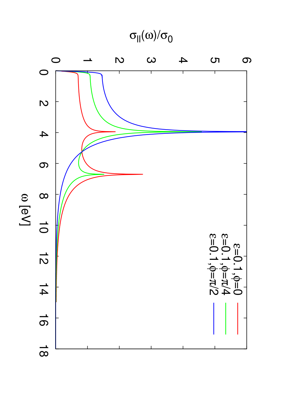
We have numerically evaluated the longitudinal optical conductivity , Eq. (29) as a function of frequency at fixed temperature eV, for several strain moduli and directions , as well as field orientations, here parametrized by the angle between the applied electric field and the lattice direction. Figs. 7 and 8 show our results in the case of strain applied in the armchair direction (). Fig. 7 shows a contour plot of the longitudinal optical conductivity as a function of frequency (radial coordinate) and applied field angle (polar angle). In the relaxed limit (), is isotropic with respect to the applied field angle, and exhibits a maximum at a frequency that can be related to the single Van Hove singularity in the DOS (cf. Fig. 4). Such a maximum is immediately split into distinct maxima, in general, as soon as the strain modulus becomes nonzero. This can be interpreted in terms of applied strain partly removing the degeneracy among the inequivalent underlying ETTs. Such an effect is however dependent on the field direction , as is shown already by the anisotropic pattern developed by in Fig. 7, for . Indeed, Fig. 8 shows plots of as a function of frequency for fixed strain modulus and varying field orientation . The relative weight of the three maxima depends on the relative orientation between strain and applied field. Here and below, we consider the case . A nonzero value of the chemical potential would result in a vanishing conductivity below a cutoff at , smeared by finite temperature effects [6].


An analogous behavior is recovered when strain is applied along the zig zag direction , as shown in Figs. 9 and 10. Again, applied strain breaks down the original isotropy of the optical conductivity with respect to the field orientation in the relaxed case, with two maxima appearing as a function of frequency (Fig. 9). The optical weight of the different maxima depend in general by the relative orientation between strain and applied field. While the presence of the two peaks can be traced back to the existence of inequivalent ETTs, whose degeneracy is here removed by applied strain, the last panel in Fig. 9 shows that at a sufficiently large strain modulus (here, ), a gap opens in the low-energy sector of the spectrum, which is signalled here by a vanishing optical conductivity (dark spot at the origin in last panel of Fig. 9).


Finally, Figs. 11 and 12 show the longitudinal optical conductivity in the case of increasing strain applied along a generic direction, viz. . Like in the previous cases, applied strain removes the isotropy of with respect to the field orientation . However, the degeneracy among the three inequivalent ETTs is here lifted completely, and three peaks in general appear in the longitudinal optical conductivity as a function of frequency, as shown also by Fig. 12. The redistribution of optical weight among the three peaks is now more complicated, as it in general depends on both the strain direction and the field orientation .
V Conclusions
We have discussed the strain dependence of the band structure, and derived the strain and field dependence of the optical conductivity of graphene under uniaxial strain. Within a tight-binding model, including strain-dependent nearest neighbour hoppings and orbital overlaps, we have interpreted the evolution of the band dispersion relations with strain modulus and direction in terms of the proximity to several electronic topological transitions (ETT). These correspond to the change of topology of the Fermi line as a function of strain. In the case of graphene, one may distinguish among three distinct ETTs. We also recover the evolution of the location of the Dirac points, which move away from the two inequivalent symmetric points and as a function of strain. For sufficiently small strain modulus, however, one may still linearly expand the band dispersion relations around the new Dirac points, thereby recovering a cone approximation, but now with elliptical sections at constant energy, as a result of the strain-induced deformation. This may be interpreted in terms of robustness of the peculiar quantum state characterizing the electron liquid in graphene, and can be described as an instance of ‘quantum protectorate’. For increasing strain, two inequivalent Dirac points may merge into one, which usually occurs at either midpoint () of the first Brillouin zone boundary, depending on the strain direction. This corresponds to the breaking down of linearity of the band dispersions along a given direction through the Dirac points, the emergence of low-energy quasiparticles with an anisotropic massive low-energy spectrum, and the opening of a gap in the energy spectrum. Besides, we confirm that such an event depends not only on the strain modulus, but characteristically also on the strain direction. In particular, no gap opens when strain is applied along the armchair direction.
We derived the energy dependence of the density of states, and recovered a linear dependence at low energy within the cone approximation, albeit modified by a renormalized strain-dependent slope. In particular, such a slope has been shown to increase with increasing strain modulus, regardless of the strain direction, thus suggesting that applied strain may obtain a steeper DOS in the linear regime, thereby helping in increasing the carrier concentration of strained samples, e.g. by an applied gate voltage. We have also calculated the DOS beyond the Dirac cone approximation. As is generic for two-dimensional systems, the proximity to ETTs gives rise to (possibly degenerate) Van Hove singularities in the density of states, appearing as logarithmic peaks in the DOS.
Finally, we generalized our previous results for the optical conductivity [36] to the case of strained graphene. We studied the frequency dependence of the longitudinal optical conductivity as a function of strain modulus and direction, as well as of field orientation. Our main results are that (a) logarithmic peaks appear in the optical conductivity at sufficiently high frequency, and can be related to the ETTs in the electronic spectrum under strain, and depending on the strain direction; (b) the relative weight of the peaks in general depends on the strain direction and field orientation, and contributes to the generally anisotropic pattern of the optical conductivity as a function of field orientation; (c) the opening of a band gap, where allowed, is signalled by a vanishing optical conductivity. Thus, an experimental study of the optical conductivity in the visible range of frequencies as a function of strain modulus and direction, as well as of field orientation, should enable one to identify the occurrence of the three distinct ETTs predicted for graphene [47].
In our study, we have assumed that the chemical potential does not itself depend on strain. In the doped case, this is clearly an approximation, as the carrier concentration is expected to remain constant, while the band structure is modified by strain. It will therefore of interest, for future studies, to investigate the strain-dependence of the chemical potential required to maintain a constant carrier concentration. This will enable one to evaluate the dependence of the Hall resistivity on uniaxial strain, which is a quantity of experimental interest [48, 49].

Appendix A Section of a Dirac cone for strained graphene
Eq. (17) yields the canonical form of the ellipse obtained as a section with constant energy of the cone approximating the band dispersions around either Dirac point , Eq. (15). The center with respect to of the ellipse evolves linearly with energy according to
| (31a) | |||||
| (31b) | |||||
The ellipse semiaxes , are given by
| (32a) | |||||
| (32b) | |||||
In the above equations, we have made use of the following definitions:
| (33a) | |||||
| (33b) | |||||
| (33c) | |||||
| (33d) | |||||
| (33e) | |||||
where is given in Eq. (16). One finds , while in the limit of no strain, . Fig. 13 shows the dependence on the strain modulus of the scaled coordinates of the ellipse center for different strain orientations.
References
- [1] K. S. Novoselov, A. K. Geim, S. V. Morozov, D. Jiang, Y. Zhang, S. V. Dubonos, I. V. Grigorieva, and A. A. Firsov, Science 306, 666 (2004).
- [2] K. S. Novoselov, A. K. Geim, S. V. Morozov, D. Jiang, M. I. Katsnelson, I. V. Grigorieva, S. V. Dubonos, and A. A. Firsov, Nature 438, 197 (2005).
- [3] A. H. Castro Neto, F. Guinea, N. M. R. Peres, K. S. Novoselov, and A. K. Geim, Rev. Mod. Phys. 81, 000109 (2009).
- [4] Y. Zhang, Y. Tan, H. L. Stormer, and P. Kim, Nature 438, 201 (2005).
- [5] C. Berger, Z. Song, X. Li, X. Wu, N. Brown, C. Naud, D. Mayou, T. Li, J. Hass, A. N. Marchenkov, E. H. Conrad, P. N. First, and W. A. de Heer, Science 312, 1191 (2006).
- [6] T. Stauber, N. M. R. Peres, and A. K. Geim, Phys. Rev. B 78, 085432 (2008).
- [7] V. P. Gusynin and S. G. Sharapov, Phys. Rev. B 73, 245411 (2006).
- [8] F. Liu, P. Ming, and J. Li, Phys. Rev. B 76, 064120 (2007).
- [9] K. S. Kim, Y. Zhao, H. Jang, S. Y. Lee, J. M. Kim, K. S. Kim, J. H. Ahn, P. Kim, J. Choi, and B. H. Hong, Nature 457, 706 (2009).
- [10] Z. H. Ni, T. Yu, Y. H. Lu, Y. Y. Wang, Y. P. Feng, and Z. X. Shen, ACS Nano 2, 2301 (2008).
- [11] T. M. G. Mohiuddin, A. Lombardo, R. R. Nair, A. Bonetti, G. Savini, R. Jalil, N. Bonini, D. M. Basko, C. Galiotis, N. Marzari, K. S. Novoselov, A. K. Geim, and A. C. Ferrari, Phys. Rev. B 79, 205433 (2009).
- [12] G. Gui, J. Li, and J. Zhong, Phys. Rev. B 78, 075435 (2008).
- [13] V. M. Pereira, A. H. Castro Neto, and N. M. R. Peres, Phys. Rev. B 80, 045401 (2009), preprint arXiv:0811.4396.
- [14] R. M. Ribeiro, V. M. Pereira, N. M. R. Peres, P. R. Briddon, and A. H. C. Neto, … …, … (2009), preprint arXiv:0905.1573.
- [15] R. B. Laughlin and D. Pines, Proc. Nat. Acad. Sci. (US) 97, 28 (2000).
- [16] V. P. Gusynin, S. G. Sharapov, and J. P. Carbotte, Int. J. Mod. Phys. B 21, 4611 (2007).
- [17] N. M. R. Peres, F. Guinea, and A. H. Castro Neto, Phys. Rev. B 73, 125411 (2006).
- [18] L. A. Falkovsky and A. A. Varlamov, Eur. Phys. J. B 56, 281 (2007).
- [19] K. F. Mak, M. Y. Sfeir, Y. Wu, C. H. Lui, J. A. Misewich, and T. F. Heinz, Phys. Rev. Lett. 101, 196405 (2008).
- [20] R. R. Nair, P. Blake, A. N. Grigorenko, K. S. Novoselov, T. J. Booth, T. Stauber, N. M. R. Peres, and A. K. Geim, Science 324, 1312 (2008).
- [21] I. M. Lifshitz, Sov. Phys. JETP 11, 1130 (1960), [Zh. Eksp. Teor. Fiz. 38, 1569 (1960)].
- [22] Ya. M. Blanter, M. I. Kaganov, A. V. Pantsulaya, and A. A. Varlamov, Phys. Rep. 245, 159 (1994).
- [23] A. A. Varlamov, G. Balestrino, E. Milani, and D. V. Livanov, Adv. Phys. 48, 655 (1999).
- [24] G. Montambaux, F. Piechon, J. Fuchs, and M. O. Goerbig, … …, … (2008).
- [25] X. Wen, Quantum Field Theory of Many-Body Systems (Oxford University Press, Oxford, 2007).
- [26] M. O. Goerbig, J. N. Fuchs, G. Montambaux, and F. Piéchon, Phys. Rev. B 78, 045415 (2008).
- [27] G. G. N. Angilella, E. Piegari, R. Pucci, and A. A. Varlamov, in Frontiers of high pressure research II: Application of high pressure to low-dimensional novel electronic materials, edited by H. D. Hochheimer, B. Kuchta, P. K. Dorhout, and J. L. Yarger (Kluwer, Dordrecht, 2001), vol. 48 of NATO Science Series.
- [28] B. Wunsch, F. Guinea, and F. Sols, New J. Phys. 10, 103027 (2008).
- [29] S. L. Zhu, B. Wang, and L. M. Duan, Phys. Rev. Lett. 98, 260402 (2007).
- [30] S. Reich, J. Maultzsch, C. Thomsen, and P. Ordejón, Phys. Rev. B 66, 035412 (2002).
- [31] M. Farjam and H. Rafii-Tabar, Phys. Rev. B …, … (2009), (submitted for publication; preprint arXiv:0903.1702).
- [32] O. L. Blakslee, D. G. Proctor, E. J. Seldin, G. B. Spence, and T. Weng, J. Appl. Phys. 41, 3373 (1970).
- [33] E. Cadelano, P. L. Palla, S. Giordano, and L. Colombo, Phys. Rev. Lett. 102, 235502 (2009).
- [34] E. Ertekin, D. C. Chrzan, and M. S. Daw, Phys. Rev. B 79, 155421 (2009).
- [35] P. W. Chung, Phys. Rev. B 73, 075433 (2006).
- [36] F. M. D. Pellegrino, G. G. N. Angilella, and R. Pucci, Phys. Rev. B 80, 094203 (2009), preprint arXiv.org/0909.1903.
- [37] C. Bena, Phys. Rev. B 79, 125427 (2009).
- [38] I. S. Gradshteyn and I. M. Ryzhik, Table of Integrals, Series, and Products (Academic Press, Boston, 1994), 5th ed.
- [39] W. A. Harrison, Electronic structure and the properties of solids (Dover, New York, 1980).
- [40] Y. Hasegawa, R. Konno, H. Nakano, and M. Kohmoto, Phys. Rev. B 74, 033413 (2006).
- [41] M. S. Dresselhaus, G. Dresselhaus, and A. Jorio, Group Theory: Application to the Physics of Condensed Matter (Springer, Berlin, 2008).
- [42] G. G. N. Angilella, E. Piegari, and A. A. Varlamov, Phys. Rev. B 66, 014501 (2002a).
- [43] G. G. N. Angilella, R. Pucci, A. A. Varlamov, and F. Onufrieva, Phys. Rev. B 67, 134525 (2003).
- [44] G. G. N. Angilella, G. Balestrino, P. Cermelli, P. Podio-Guidugli, and A. A. Varlamov, Eur. Phys. J. B 26, 67 (2002b).
- [45] H. Bruus and K. Flensberg, Many-Body Quantum Theory in Condensed Matter Physics: An Introduction (Oxford University Press, Oxford, 2004).
- [46] I. Paul and G. Kotliar, Phys. Rev. B 67, 115131 (2003).
- [47] F. M. D. Pellegrino, G. G. N. Angilella, and R. Pucci, High Press. Res. 30, … (2010).
- [48] X. Zotos, F. Naef, M. Long, and P. Prelovšek, Phys. Rev. Lett. 85, 377 (2000).
- [49] P. Prelovšek and X. Zotos, Phys. Rev. B 64, 235114 (2001).