Infrared Diagnostics for the Extended 12 m Sample of Seyferts
Abstract
We present an analysis of Spitzer IRS spectroscopy of 83 active galaxies from the extended 12m sample. We find rank correlations between several tracers of star formation which suggest that (1) the PAH feature is a reliable tracer of star formation, (2) there is a significant contribution to the heating of the cool dust by stars, (3) the H2 emission is also primarily excited by star formation.
The 55-90 vs. 20-30 spectral index plot is also a diagnostic of the relative contribution of Starburst to AGN. We see there is a large change in spectral index across the sample: for both indices. Thus, the contribution to the IR spectrum from the AGN and starburst components can be comparable in magnitude but the relative contribution also varies widely across the sample.
We find rank correlations between several AGN tracers. We find correlations of the ratios [OIII]5007/[OIV]26m and [OIII]5007/[NeV]14m with the Sil strength which we adopt as an orientation indicator. This suggests that some of the [OIII]5007 emission in these Seyferts is subject to orientation dependent obscuration as found by Haas et al. [40] for radio galaxies and quasars. There is no correlation of [NeV] EW with the Sil 10m strength indicating that the [NeV] emission is not strongly orientation dependent. This suggests that the obscuring material (e.g., torus) is not very optically thick at 14m consistent with the results of Buchanan et al. [10].
We search for correlations between AGN and Starburst tracers and we conclude that the AGN and Starburst tracers are not correlated. This is consistent with our conclusion that the relative strength of the AGN and Starburst components varies widely across the sample. Thus, there is no simple link between AGN fueling and Black Hole Growth and star formation in these galaxies.
The density diagnostic [NeV] 14/24 m and [SIII] 18/33 m line ratios are consistent with the gas being near the low density limit, i.e., cm-3 for [NeV] and few hundred cm-3 for [SIII].
The distribution of Sil 10 m and 18 m strengths is consistent with the clumpy torus models of Sirocky et al. [82].
We find a rank correlation between the [NeV] 14m line and the 6.7 m continuum which may be due to an extended component of hot dust.
The Sy 2’s with a Hidden Broad Line Region (HBLR) have a higher ratio of AGN to Starburst contribution to the SED than Sy 2’s without an HBLR. This may contribute to the detection of the HBLR in polarized light. The Sy 2’s with an HBLR are more similar to the Sy 1’s than they are to the Sy 2’s without an HBLR.
Keywords:
galaxies: active - galaxies: Seyfert - galaxies: spiral - infrared: galaxiesI Introduction
The basic paradigm for nuclear activity in galaxies, an accretion disc around a super massive black hole (SMBH), is well-established. However, we have at best a sketchy understanding of how SMBH are formed and what role nuclear activity plays in galaxy evolution. As we learn more about the formation and evolution of normal galaxies, and better understand the physics of active galactic nuclei (AGNs), it is becoming clear that these processes are intimately connected. The ubiquity of super massive black holes and the observed relation between black hole mass and bulge mass [61, 33] suggest that nuclear activity may be closely connected to star formation in all galaxies. Accretion onto a black hole, which powers AGNs, requires available fuel in the nuclear region. Gas infall is also likely to be associated with bursts of star formation [42, 62]. Furthermore, AGNs deposit energy in the surrounding interstellar medium (ISM) via ionizing radiation, radio jets and perhaps winds, possibly triggering star formation. Circumnuclear star formation has been observed in AGN and a link between nuclear activity and star formation is also supported by a recent finding that the mean stellar age of narrow-line AGNs is much younger than in similar normal spiral galaxies [47]. However, the interaction between active nuclei and their host galaxies remains poorly understood.
The mid-IR includes important diagnostics such as the PAHs, Sil features, and fine structure lines [87, 103, 34, 54]. Previous mid-IR spectroscopic studies of AGN have shown that these diagnostics allow separation of AGN and starburst properties, as well as provide constraints on orientation and obscuration of the central torus [34, 54, 14, 91, 40, 104, 67, 77, 41, 89].
This paper is part of a series on a Spitzer study of the Extended 12m Sample of Seyfert galaxies. Buchanan et al. [10] presented low resolution IRS spectra of the first 51 (of 83) sources and demonstrated the variety of mid-IR spectral shapes due to the relative mix of comparable contributions from starburst and AGN. They examined the ratio of IR to nuclear radio flux density and showed that the ratio is a factor of two larger in Sy 1’s than Sy 2’s between 15 and 35 m suggesting the torus emission is anisotropic by a factor of two at these wavelengths. Additional preliminary results have been presented by Buchanan et al. [11]. Other papers currently planned in the series will present (1) an atlas of all the data [31], (2) models of the mid- to far- IR SEDs which combine both starburst and AGN contributions [32], and (3) UKIRT observations of the near-IR emission and discuss constraints on the relative mix of starburst and AGN contributions to the spectrum [12]. In this paper we examine diagnostic features (PAH, Sil, fine structure lines, H2, continuum slope) in the IRS spectra and discuss the implications for the AGN-Starburst connection and obscuration of the central engine. We note that independent groups have also published results based on our data. Maiolino et al. [58] used observations of some Sy 1’s from Buchanan et al. [10] as a comparison sample for their study of high luminosity QSOs. Deo et al. [18] obtained low resolution Spitzer IRS observations of 12 Sy 1.8 and 1.9 and combined the results with archival data of 57 Sy 1’s and Sy 2’s from Buchanan et al. [10] and Weedman et al. [104]. High resolution IRS observations of a subsample of 29 sources are presented by Tommasin et al. [96]. Recently Wu et al. [108] published a study of 103 Seyferts which included our IRS data. Gallimore et al. [31] show that there are systematic differences between our values for the PAH and Sil features and those of Wu et al. [108] which are due to the different analysis techniques used (PAHFIT vs. Spline-fitting). Nevertheless, we agree on the overall trends which are common to both papers.
II Spitzer Observations
II.1 The Sample of AGN
The properties of the sample are discussed by Buchanan et al. [10] and Gallimore et al. [31]. The sample comprises all galaxies identified as Seyferts or LINERS from the extended 12 µm sample of Rush et al. [74] that have km s-1. The potential advantage of the 12 µm sample is its perceived resistance to wavelength-dependent selection effects [86]. Note that there may in fact be selection effects in the sample due to anisotropic emission from the torus at 12 µm [10]. The redshift criterion was included to ensure that the smallest possible physical size was probed by the fixed Spitzer apertures in order to better exclude host galaxy emission. The data include IRAC imaging, IRS spectral mapping, and MIPS SED spectra as described by Gallimore et al. [31].
The spectral classifications were obtained by a thorough search of the literature for each galaxy; see Table 1 of Gallimore et al. [31]. For the purposes of comparing the Seyfert types we consider Seyfert types 1. (i.e. types 1.0, 1.2, 1.5, 1.8, and 1.9 as well as narrow line Seyfert 1’s) to be Sy 1’s, and objects with no broad permitted lines to be Sy 2’s. We consider the properties of the Seyferts with hidden broad line regions (HBLRs) separately and compare them to the Sy 1’s and Sy 2’s. We refer to the sum of the Sy 1’s, Sy 2’s, and hidden Sy 1’s as the combined sample. The resulting sample contains 83 sources of which 7 are now classified as HII galaxies, 6 are LINERS and the remaining 70 are Seyferts (27 Sy 1-1.5, 17 Sy 2 with HBLR, 20 Sy 2 without HBLR, and 6 Sy 1.8-1.9. The sample is listed in Table 1 of Gallimore et al. [31].
II.2 IRS Observations and Data Reduction
The sample galaxies were observed by Spitzer IRS [44] in spectral mapping mode, using the Short-Low and Long-Low modules. The modules cover a wavelength range of 5 – 36 µm, with a resolving power () ranging from 64 to 128. The integration times were 6 seconds per slit pointing. Details of the observing and reduction are given by Gallimore et al. [31] and are summarized here.
The spectral maps were constructed to span in the cross-slit direction and centered on the target source. The observations were stepped perpendicular to the slit by half slit-width spacings. For the SL data, the mapping involved 13 observations stepped by 1.8” perpendicular to the slit, and for the LL data, 5 observations stepped by 5.25” perpendicular to the slit. The resulting spectral cubes span roughly 25.3” x 54.6” (5.3 - 14.2 m) for the SL data and 29.1” x 151” (14.2 - 36 m) for the LL data.
The raw data were processed through the Spitzer BCG pipeline, version S15.3.0. Sky subtraction employed off-source orders. In SL and LL observations, the source is centered in first or second order separately, with the “off-order” observing the sky at an offset position along the slit orientation. Sky frames were constructed using median combinations of the off-source data and subtracted from the on-source data of matching order. No detectable contamination appeared in the sky frame images.
Data cubes were constructed and edited for cosmic-rays and spurious pixels using the CUBISM software package developed by the SINGS IRS team [85]. We used synthetic, 20” diameter circular apertures to extract the spectra.
To calibrate the flux scale, we employed archival IRS staring and spectral mapping observations of the calibrator stars HR7341 (SL) and HR6606 (LL). The staring mode spectra were extracted using SPICE (Spitzer Science Center 2006), and the spectral mapping observations were processed as described above. The flux calibration curve was determined by the ratio of the flux-calibrated staring mode spectra to the uncalibrated cube-extracted spectra. This flux calibration was applied to all target sources observed in spectral mapping mode. Based on inspection of the spectral overlaps between modules and orders the calibration is self-consistent to within 5% across the IRS spectrum. The only exception was NGC 4151, SL order 1, which had to be scaled down by to match the neighboring SL order 2 and LL order 2 spectra, perhaps owing to a residual pipeline error. After applying a uniform scaling to SL order 1, the spectrum matched well the neighboring spectral overlaps.
Archival data of our sample, such as obtained by the SINGS collaboration, were processed in the same manner. There are however a few sources for which only staring mode observations are available for the SL module: NGC 526A, NGC 3227, NGC 4941, IC 5063, NGC 7172, and NGC 7314. The staring mode spectra were extracted using SPICE and scaled to match IRAC 5.8 and 8.0 m photometry obtained as part of this project [31].
II.3 MIPS-SED Observations and Data Reduction
The sample galaxies were also observed using the MIPS camera in SED mode, which provides very low resolution () slit spectroscopy covering –90 m. The slit-width for SED mode observations is 20″. Integration times ranged from 3 to 10 seconds depending on the IRAS 60m flux density. Observations include six pairs of on-source and off-source positions (1-3′ away from source) for background subtraction.
Basic data processing, including background subtraction and flux and wavelength calibration, was handled by the Spitzer pipeline (version S.14.4). The final, low resolution spectra were extracted from the long-slit images using a three-pixel (″) synthetic aperture perpendicular to the slit. For each source, the position of the galaxy nucleus was identified first manually and then by a Gaussian fit to determine the center of the extraction aperture to a fraction of a pixel.
Note that flux calibration is derived from observations of standard stars and so is most accurate for compact far-infrared sources. Formally, the accuracy for point sources is better than 10%, but degrades to % for extended sources with galaxy-like surface brightness profiles [56].
II.4 PAHFIT Spectral Decomposition
We used the PAHFIT spectral decomposition code [84] to fit and extract line features of the Seyfert IRS spectra. The publicly available release of PAHFIT permits silicate features only in absorption. Silicate 10 m and 18 m emission commonly appears among the sample, however, and we therefore modified PAHFIT to include a warm, optically thin () dusty medium. To accommodate the range of observed Sil emission profiles, the warm dust model includes two components: (1) an optically thin warm medium, characterized by a single temperature and 10 m opacity, and (2) a cold, partially covering dusty medium parameterized solely by covering fraction (i.e., the cold dust is modeled to produce no significant emission over the IRS band). Both the cold and warm dust components obey the extinction law described by Smith et al. [84]. Our goal was to reproduce the observed silicate emission profile shapes without regard to determining the physics of the warm dust (other than its presence and emission strength), and so, for simplicity, the spectrum of the warm dust, modified by partial foreground absorber, was calculated assuming a simple slab geometry.
Except for this added warm dust component, we used PAHFIT with its default settings. PAHFIT robustly decomposes the spectrum into multiple temperature dust components, silicate features, emission lines, and PAH dust features. The decomposition proceeds using a standard non-linear fitting algorithm. PAHFIT was specifically designed to analyze moderate resolution IRS spectra and carefully limits parameters, such as line widths and centroids, that might drift to unphysical values during the fit.
The final data products include tables of line strengths and equivalent widths. We further modified PAHFIT to produce line-subtracted continua. These continua were used to calculate silicate strengths and spectral indices. In addition, we also modified the PAHFIT output to produce 3 upper limits for weak or undetected lines. These data tables are provided in Gallimore et al. [31]. Note that the line and feature fluxes are not corrected for extinction.
Table 1 summarizes the results of the PAHFIT decomposition, giving the median values of a range of properties for the continuum emission, Sil feature, star formation tracers, AGN tracers, and diagnostic line ratios. The median values were calculated based on the computation of a survival curve [27]. As the line ratios include both upper and lower limits, we employed the formalism for interval-censoring given by Finkelstein [28] and Sun [93], as implemented in the interval package by M. P. Fay & P. A. Shaw (http://cran.r-project.org/web/packages/interval/index.html).
Tables 2-9 give the results of statistical tests for the significance of differences in the distribution of those properties for the different Seyfert subgroups. These tests comprise Kolmogorov-Smirnov two-sample tests for uncensored data, or log-rank tests for interval-censored data.
Table 10 gives the significance of rank correlations between the properties for the combined sample. We used Kendall’s rank correlation statistic adapted for interval-censored data [46], reported as a -score and two-sided significance level.
In this paper, we search extensively for patterns in the data by exploring bivariate correlations among measurements: for example, PAH eqw vs. 20–30 m spectral index. There are well-known parametric and non-parametric statistical measures of correlation (see, e.g., Sprent & Smeeton 90). Parametric methods specifically apply to cases where the data are believed to be related through some known and prescribed functional form; for example, the well-known Pearson correlation coefficient measures the underlying linear relationship between measurements. One however expects a fairly complex relationship, if at all, between a spectral index and an eqw, and so such parametric statistics would not be expected to apply in the present analyses. For example, data that are tightly but non-linearly correlated will likely show low linear correlation measurements [5].
In contrast, rank correlation coefficients provide a robust, non-parametric measure of association between measurements. They are better suited for the present study, as they measure simply the degree to which one measurement increases (or decreases) as another increases, independent of the degree or functional form of the underlying association. To our knowledge, only Kendall’s rank correlation statistic (Kendall’s ; [48]) has been generalized to account both for upper limits (non-detections) and lower limits (e.g., line ratios where the divisor is an upper limit) in one or both measurements and so is ideal for this study. We have implemented the generalized Kendall’s rank correlation statistic following the formalism of Isobe, Feigelson, & Nelson [46]. In the results tables, we report the standard normal score () of the statistic as well as the probability () that score would have occurred by chance (i.e., the probability of no correlation). We chose to be conservative in the interpretation of the correlation statistics and adopt the threshold to indicate evidence of rank correlation.
III RESULTS
III.1 The Starburst AGN Connection
III.1.1 PAH Emission as a diagnostic of Star Formation
The PAH emission is thought to be produced when small grains (containing Carbon atoms) are heated by single UV photons from hot stars and radiate though their vibrational modes [95]. It is clear that PAH emission is a tracer of star forming regions in our Galaxy [95] and other galaxies [54, 70, 8, 16, 21, 84] The PAH luminosity is proportional to the star formation rate in star forming galaxies [73, 8, 13, 78, 26]. Voit [102] argues that PAH grains exposed to the direct hard continuum of an AGN will be destroyed, and the PAHs in AGN can only survive when they are shielded by high columns of X-ray absorbing gas, e.g., in the plane of the obscuring torus. Smith et al. [84] notes that the ratio of 7.7/11.3 micron PAH seems to be lower in some AGN than in starburst galaxies. Since the 11.3 micron PAH are produced by larger grains than the 7.7 micron PAH [20] this suggests that the smaller grains are indeed being destroyed by the AGN. Thus, PAH emission seems to be a good indicator of star formation in galaxies with the caveat that it may be significantly suppressed in AGN. Siebenmorgen, Krügel & Spoon (2004) compare radiative transfer models which include dust destruction for starbursts and AGN. In their models, some PAH emission is produced within clouds illuminated by an AGN, but the strength of the PAH is lower by a factor of about 5 than that produced in the starburst models with the same luminosity and Av. Finally, the equivalent width of PAH features has been shown to be useful in diagnostic diagrams as a discriminant between starbursts and AGN as the energy source for infrared emission [34, 54, 70, 6, 89].
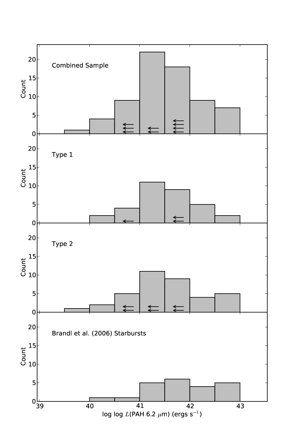
The 6.2 micron PAH feature is thought to be relatively “unconfused” by other spectral features (e.g., Peeters et al. 2004) and so should be a good measure of the amount of star formation. We show the distribution of 6.2 m PAH EW for the Sy 1’s, Sy 2’s and hidden Sy 1’s in Figure 1. We see that the Sy 2s show a distribution to higher values of PAH EW. We find that the distribution of PAH EW in the Sy 1’s and Sy 2’s are significantly different (Table 2) in contrast to Wu et al. [108] who find no significant difference in the EWs. This might be due to the systematic differences in the measured PAH EWs discussed by Gallimore et al. [31]. The Sy 2’s which show the high EW are those without an HBLR; the Sy 2’s with an HBLR have a distribution which is similar to that of the Sy 1’s (Tables 1, 2,3). The higher values of PAH EW for the Sy 2s seems mainly due to the lower continuum fluxes in the Sy 2’s relative to the Sy 1’s since the PAH luminosities (Figure 2) are similar in the Sy 2’s and the Sy 1’s. This result is consistent with the findings of Clavel et al. (2000) for a sample of Seyferts studied using ISO. Figures 1 and 2 also show that the Seyferts show a similar distribution in 6.2 m PAH luminosity as the Brandl et al. [8] starbursts. However, the Seyferts show lower 6.2 m PAH EW due to the higher continuum contribution from the AGN. These results are consistent with the results of Buchanan et al. [10] that principle component analysis required a higher star formation contribution to the SED of Sy 2’s.
III.1.2 The PAH 6.2/11.3 ratio
The 6.2 m PAH feature is produced by grains with smaller sizes than the 11.3 m PAH feature [20]. The smaller grains are more quickly destroyed by exposure to the AGN spectrum. Thus, the ratio of 6.2/11.3 PAH should be an indicator of the destruction of grains by the AGN [84]. Wu et al. [108] show that their Seyfert sample and the Brandl et al. [8] sample of starburst galaxies have similar average values for the 11.3/6.2 PAH ratio.
We calculate the 6.2/11.3 PAH ratio using the fluxes of the features. The distribution of the 6.2/11.3 PAH ratio is consistent with being the same in the different subgroups. In Figure 3 we plot the ratio of the 6.2 and 11.3 m PAH strength vs. the [NeV] luminosity which traces the strength of the AGN ionizing continuum (§ III.1.6). We see no correlation of the PAH ratio with the [NeV] luminosity. In Figure 4 we plot the 6.2/11.3 PAH ratio against the Sil 10 m Strength (see §III.2.1). We do not see a correlation between the PAH ratio and the Sil 10 m Strength (Table 10). This suggests that the PAH emission that we see in these Seyferts is not orientation dependent. Any effect of the AGN on the distribution of PAH grains must be confined to a small volume so that the integrated measurements studied here are not affected.
III.1.3 PAH Associated with Emission from Cool Dust
Schweitzer et al. [76] show that QSOs and ULIRGs lie on the same correlation between 7.7 m PAH flux and 60 m continuum flux, suggesting that the FIR is dominated by dust heated by star formation. In Figure 5 we show a strong rank correlation between 6.2 m PAH luminosity and the integrated luminosity (from IRAS) at 60 m for our sample. We also find a rank correlation between the flux of the 6.2 m PAH feature and the 60 m continuum (Table 10).
We also show the 6.2 m PAH EW vs. the spectral index of the MIPS SED 55-90 m in Figure 6. The slope of the MIPS SED indicates the relative importance of cold vs. warm dust to the FIR SED. Positive slope is a red MFIR SED. The starburst galaxies all lie at large PAH EW. In the combined sample, we see a rank correlation between PAH EW and MIPS slope, with higher PAH strength (more star formation) proportional to more positive (redder) MIPS slope (more emission from cool dust). These two correlations (Figures 5 and 6) are consistent with a significant contribution from stars to the heating of the cool dust which produces the FIR emission in our sample.
III.1.4 PAH EW vs. 20-30 m spectral index: a measure of the relative strength of the starburst and AGN components
20 microns is just redward of the “knee bend” we see in the SED of many Sy 1s and 2s [10]. The 20-30 micron spectral index , was determined using a power law fit to the line-subtracted continuum between 20 and 30 microns rest frame. This spectral index characterizes the relative contribution of warm and cool dust to the mid-IR. Note that the values of used in Buchanan et al. [10] are actually + 2.0. The correct values of are used here. The similar 15-30 m spectral index has also been found to be an effective AGN discriminator [8, 15]. Using a subset of our data, Deo et al. [18] show that there is a correlation between the 6.2 m PAH EW and . Wu et al. [108] also find a correlation between the the 11.3 m PAH EW and the 15-30m spectral index. We plot the 6.2 m PAH EW vs. in Figure 7. We see the different subsamples tend to lie in different parts of the diagram. The Sy 1’s and Sy 2’s with an HBLR generally have and cover a large range in 6.2 m PAH EW. On the other hand the Sy 2’s and Liners tend to have high values of 6.2 m PAH EW and cover a large range in with the Sy 2’s showing a strong rank correlation () between the two properties. We also see a rank correlation between 6.2 m PAH Luminosity and (Figure 8). Thus we see rank correlations between the PAH EW and which are both measures of the relative strength of the starburst and AGN components, and also PAH luminosity (a measure of the absolute strength of the starburst component) and .
In Figure 7 the sources in the lower left are those with a low starburst to AGN ratio. Thus, the value of between -1 and -2 is likely to represent the spectrum of the “torus”, consistent with values calculated by Nenkova et al. [65].
In Figure 9 we plot the 55-90 m spectral index vs. 20-30 m spectral index. We see a correlation in the sense that objects which are redder in 20-30 tend to be redder in 55-90. This is consistent with the hypothesis that star formation contributes to both the 20-30 and 55-90 spectral regions. Thus, the 55-90 vs. 20-30 spectral index plot is also a diagnostic of the relative contribution of Starburst to AGN. We see there is a large range in spectral index across the sample: for both indexes. Thus, the contribution to the IR spectrum from the AGN and starburst components can be comparable in magnitude but the relative contribution also varies widely across the sample (see also Buchanan et al. 10, Deo et al. 18, Wu et al. 108).
III.1.5 The Relationship between Molecular Hydrogen and Star Formation
Figure 10 shows the 6.2 m PAH EW vs. the H 17 m EW. The H line has higher EW in the Starbursts and Liners than the Seyferts. The distribution of the fluxes and luminosities of the H 17 m line are consistent with being the same in the subclasses of Seyferts (Tables 2-8).
We see that the H EW is proportional to the PAH EW. Tommasin et al. [96] show a correlation between the luminosities of the 11.3 m PAH and H 17 m lines in a subsample of these sources. We also find a rank correlation between the luminosities of the 6.2 m PAH and the H 17 m line (a rank correlation is also found in the fluxes; Table 10). We note that Schweitzer et al. [76] have also reported a correlation between PAH and H2 in the higher luminosity QUEST QSOs. Since the PAH is a tracer of star formation this suggests that the H2 line is also associated with star formation.
In Figure 11 we plot vs. the H 17 m EW. We see a correlation in the sense that objects with redder continuum slopes have larger H EW. Since red continua are associated with cold dust from stars, this correlation is also consistent with the molecular hydrogen line being associated with star formation.
III.1.6 AGN Tracers
Following Voit [103] and Spinoglio & Malkan [87], we adopt the high ionization lines [NeV] (97.1 eV) and [OIV] (54.9 eV) as tracers of the AGN in these objects. The vast majority of stars do not produce photons sufficiently energetic to excite [NeV] and [OIV], with the exception of young Wolf-Rayet stars [75]. However, Abel & Satyapal [1] show that even in AGN with a strong starburst component, the observed ionization parameters constrain the [NeV] emission to be dominated by the AGN.
It is also possible for [NeV] and [OIV] to be excited by shocks with velocities km s-1 [4]. However, as Allen et al. note, the predicted line ratios are not in agreement with observations. Detailed studies of the IR spectrum of Seyferts are instead consistent with AGN photoionization of the NLR [37]. In addition, the line ratios [NeV]/[NeII] and [OIV]/[NeII] have proved empirically to provide good separation between AGN and Starbursts [34, 91, 92]. And the [OIV]26m line has also shown to be correlated with other AGN tracers - the [OIII]5007 line, radio emission, and the 2-10 keV X-ray flux in other samples [60, 19].
In Figure 12 we show a rank correlation between the luminosity of the [NeV] 14m line and the 8.4 GHz radio continuum. A rank correlation is also present between the fluxes of the [NeV] 14m line and the 8.4 GHz radio continuum (Table 10). The 8.4 GHz radio emission is not orientation dependent [94] and is an unbiased measure of the isotropic AGN luminosity. The rank correlation of the [NeV] 14 m line with the 8 GHz radio emission suggests that the [NeV] line emission is also a useful measure of AGN luminosity (see also § III.2.3).
In models of the obscuring torus, the flux in the near-mid IR (i.e., m) is due to hot dust heated by the AGN [72, 35, 24, 98, 64, 65]. Thus, we adopt the 6.7 m continuum flux as an AGN tracer. In § III.2.4 we show a rank correlation between the 6.7 m continuum and the [NeV] 14 m line emission.
In Figure 13 we see rank correlations between the luminosities of the two IR AGN tracers the [NeV] 14m and [OIV] 26m lines with the optical [OIII]5007 line ([OIII] measurements taken from [7, 18, 17, 38, 49, 51, 52, 60, 69, 83, 97, 100, 107, 105, 109]). The rank correlations are also present but weaker between the fluxes of the lines. This confirms that the [NeV] 14m and [OIV] 26m are useful AGN tracers.
III.1.7 Comparison of Starburst and AGN Tracers
Correlations between AGN and starburst tracers have been found for QSOs [39, 76, 66, 58] and Seyferts [58]. Figure 14 shows a rank correlation between the luminosities of the 6.2 m PAH and the [NeV] 14 m line in the combined sample. We also find rank correlations between the luminosities of (1) the 6.2 m PAH and the [OIV] 26 m line (2) the [NeV] 14 m line and the 60 m continuum, and (3) the 6.2 m PAH feature and the 6.7m continuum (not plotted, see Table 10). These correlations seem to indicate that the starburst and AGN luminosities are correlated in these Seyferts. However, our statistical tests (Table 10) show that there are no significant correlations in the flux of these AGN and Starburst tracers. Figure 15 shows that the fluxes of the 6.2 m PAH and [NeV] 14 m line scatter over an order of magnitude and are uncorrelated. So although AGN tracers are internally correlated in both flux and luminosity, and Starburst tracers are are internally correlated in both flux and luminosity, the fluxes of the AGN and Starburst tracers are not correlated. We conclude that the correlations in Starburst and AGN luminosity are due to the dependence on distance and are not real. This is consistent with our results that the relative strength of the AGN and Starburst components in these Seyferts vary widely across the sample (§ III.1.4). The lack of a correlation between the AGN and star burst suggests that in these AGN there is no direct link between AGN fueling, black hole growth, and star formation.
III.1.8 The [NeV]/[NeII] ratio vs. PAH EW Diagram
Genzel et al. [34] showed that a diagram which plots the ratio of a high to low ionization line vs. a PAH EW is able to separate Starbursts from AGN from ULIRGs. Genzel et al. [34] used [OIV]/NeII] vs. the 7.7m PAH EW. In Figure 16 we plot 6.2m PAH EW vs. [NeV]14m/[NeII]12m. We see that there are significant differences across our sample with objects with higher AGN to starburst ratio in the lower right and the objects with lower AGN to starburst ratio in the upper left. Note that the Liners have low [NeV]14m/[NeII]12m and tend to fall to the left of the other objects.
III.2 Orientation, Obscuration, and Constraints on the Torus
III.2.1 6.2 m PAH vs. Sil 10 m Strength
The strength of the Sil 10 m feature is potentially a powerful probe of the absorbing material [72, 53, 55, 45]. We adopt the definition of Sil strength given by Spoon et al. [89],
| (1) |
where is the observed flux in the feature and is the interpolated continuum flux at 10 m. Recent Spitzer results suggest that different types of objects show systematically different Sil 10 m strength [77, 41] with QSOs showing strong Sil emission, Sy 1s showing mostly weak Sil emission, Sy 2s showing mostly weak to moderate Sil absorption, and ULIRGS showing strong Sil absorption. Spoon et al. [89] have shown that objects fall mainly in two branches on the 6.2 m PAH vs. Sil 10 m Strength diagram.
Figure 17 shows the distribution on the 6.2 m PAH vs. Sil 10 m Strength diagram. Our results are consistent with those of Spoon et al. [89]. As expected, the Sy 1’s tend to show weak Sil emission, and the Sy 2’s tend to show Sil absorption. The KS test (Table 2) confirms that the distribution of Sil strength is very different in the Sy 1’s and Sy 2’s. These results are in qualitative agreement with Wu et al. [108], though as discussed by Gallimore et al. [31] there are systematic differences in the measured Sil strengths. The only significant difference between the Sy 1’s and the Sy 2’s with an HBLR is the Sil strength (Table 5).
Two of the HBLR Sy 2’s show Sil emission - F01475-0740 and M-3-58-7. In these objects, the obscuring material (torus) may be oriented at an intermediate inclination. In addition, four objects classified as S1.8-1.9 show Sil absorption - NGC1194 (S1.9), M-2-40-4 (Sy1.9), NGC1365 (S1.8), and NGC5033 (S1.8). These are also likely to be fairly edge-on (§ III.3). About half of the objects identified as Liners and Starbursts show weak Sil features, with strong absorption seen in MRK938 (HII), NGC3079 (LINER), NGC5005 (LINER), and strong emission seen in NGC4579 (LINER), NGC5494 (LINER), and CGCG381-051 (HII).
III.2.2 Sil 10 m Strength vs. Sil 18 m Strength
Sirocky et al. [82] showed that the observed relationship between the two Sil features 18 m and 10 m can be a powerful probe of the properties of the obscuring material. Figure 18 shows the distribution of the Sil strengths for the different subsamples of galaxies. We see the Sy 1’s mainly to the upper right with emission in both Sil features, and the Sy 2’s mainly to the lower left with absorption in both Sil features. In Figure 19 we compare our results for the two Sil Strength features with simple spherical obscuration models [82]. The spherical models have the advantage that they reduce the number of free parameters and still give good agreement with the more detailed clumpy torus models [64, 65]. We see that the data lie below the smooth torus models and within the parameter space of the clumpy torus models. Our data are inconsistent with the smooth torus models but are consistent with the clumpy torus models. Within the context of the spherical clumpy models, there is a preference for a small number of clumps along the line of sight ().
III.2.3 Density and Obscuration Diagnostics
The [NeV] 14/24 and [SIII] 18/33 line ratios are density diagnostics [103, 87], and in principle, in the low density limit can be used as extinction indicators [103, 3, 22]. The [NeV] lines will probe high excitation gas, most likely in the narrow line region, while the [SIII] can be excited by stars and may be produced on a larger spatial scale. Sturm et al (2002) examined the [NeV] 14/24 ratio in a sample of Seyferts using ISO data and also concluded that the [NeV] emitting gas in both Seyfert types was in the low density limit. On the other hand Dudik et al. [22] find that type 2 AGNs tend to have lower ratios than type 1 AGN, and some of the type 2 AGNs are below the low density limit possibly due to differential absorption. Tommasin et al. (2008) using high resolution IRS spectra on a subsample of the 12 m sample, report [NeV] line ratios slightly above the low density limit, giving densities of cm-3.
Our data (Figure 20) and Tables 1 - 5) are consistent with Sy 1’s, Sy 2’s and hidden Sy 1’s having the same distribution of these diagnostic ratios. Both line ratios seem to scatter around their low density values giving for [NeV] cm-3 and for [SIII], few hundred cm-3. We also see no evidence for a correlation between the values of these ratios (Table 10).
In Figure 21 we plot the [NeV] 14/24 line ratio against the Sil 10 m feature which is an indicator of absorption along the line of sight (§III.2.1). We see that there is no correlation between these two quantities (Table 10). This suggests that extinction does not have a significant effect on the observed [NeV] 14/24 line ratio.
In Figure 22 we show the [NeV] 14 m EW vs. Sil 10 m Strength. We see that the distribution of [NeV] EW is similar in Sy 1’s, Sy 2’s and hidden Sy 1’s (Table 2, 3,4,5). There is no correlation of [NeV] EW or luminosity with Sil strength (Table 10). This is consistent with our results above that (1) the [NeV] luminosity is proportional to the radio power, and (2) the effect of extinction on the [NeV] 14/24 ratio is small. This suggests that either the torus is not very opaque at these wavelengths (14-24 m), or [NeV] is produced primarily outside the torus, e.g., in the NLR. However, we expect the high ionization lines [NeV] and [OIII] to be produced in similar locations around the AGN.
Haas et al. [40] have shown that [OIII] is very orientation dependent in quasars and radio galaxies, suggesting that much of the [OIII] is produced in regions obscured by the torus. In Figure 23 we show the ratios [OIII]5007/[OIV]26m and [OIII]5007/[NeV]14m vs. the Sil Strength. We see a strong rank correlation for [OIII]5007/[OIV]26m and a weaker one for [OIII]5007/[NeV]14m in the sense that the ratio is higher in objects with Sil emission (roughly face on) and lower in objects with Sil absorption (roughly edge on). We find that [OIII] is orientation dependent in our sample of Seyferts suggesting that much of the [OIII] emission is produced in a region which is subject to orientation dependent obscuration, e.g., the torus. Thus, if [NeV] is also primarily produced in regions obscured by the torus, then our result suggests that the opacity of the torus at 14 m is not large. This is consistent with the results of Buchanan et al. [10].
III.2.4 An Extended Hot Dust Component in Seyferts?
High resolution mid-IR observations show extended hot dust associated with the NLR in NGC1068 (Galliano et al. 2005; Mason et al. 2006) and the Circinus galaxy (Packham et al. 2005). Figure 24 shows a rank correlation between the luminosities in the [NeV] 14m line and the continuum determined at 6.7 m in our Seyferts. The rank correlation is also present between the fluxes (Table 10). In § III.2.3 we show that the [NeV] emission is not strongly orientation dependent. However, in models where the 6.7 m continuum originates in the hot dust in the inner torus, we would expect the 6.7 m continuum to be orientation dependent. In the context of standard uniform torus models we would expect that the 6.7 m emission should be high in the Sy 1’s, but low in the Sy 2’s where it is obscured by the torus. Instead we see a strong rank correlation followed by both Sy 1’s and Sy 2’s. This suggests that in addition to any hot dust in the torus, we are seeing an extended component of hot dust whose luminosity scales with the AGN luminosity (as measured by [NeV]). This might be due to dust in the NLR or a wind. Mor et al. [63] also find evidence for hot dust emission associated with the NLR in luminous QSOs.
III.3 Comparison of Seyfert Subsamples
Here we discuss the properties of subsamples of the Seyfert population. Table 1 gives the median values of a range of properties for the continuum emission, Sil feature, star formation tracers, AGN tracers, and diagnostic line ratios. Tables 2-9 give the results of statistical tests for the significance of differences in the distribution of those properties.
The comparison of the Sy 1’s with the Sy 2’s (both with and without a detected HBLR) (Table 2) shows significant differences () between the Sil feature, the 20-30 m spectral index, 6.7 m continuum flux density, and the EW of the 6.2 m PAH feature. As discussed in §III.2.1, the Sy 1’s exhibit weak Sil emission and the Sy 2’s show Sil absorption. The other differences are consistent with being due to a higher contribution from hot dust in the spectra of the Sy 1’s which causes higher 6.7 m continuum, bluer 20-30 m spectral index, and lower EW of the 6.2 m PAH feature. Note that although the EWs are different, the luminosities are similar. When we compare the Sy 1’s to just those Sy 2’s without an HBLR (Table 3) we see the same differences as between the Sy 1’s and all the Sy 2’s, with the addition of a difference in the luminosity of the 6.7 m continuum.
The Sy 2’s with and without HBLRs show differences in 20-30 m spectral index, 6.7 m continuum, and EW of the 6.2 m PAH feature and the H line (Table 4). These differences are consistent with a higher contribution from a hot dust component in the HBLR Sy 2’s. In addition, the Sy 2’s with an HBLR are very similar to the the Sy 1’s; the only significant difference is the Sil strength (Table 5). Thus, the Sy 2’s with an HBLR are more similar to the Sy 1’s than they are to the Sy 2’s without an HBLR. The differences are in the sense that the Sy 2’s with an HBLR have a higher ratio of AGN to Starburst contribution to the SED. This may contribute to the detection of the HBLR in polarized light. This is consistent with Alexander [2] who noted that there was a weaker contribution from the galaxy in the HBLR Sy 2’s than the non-HBLR Sy 2’s. We cannot rule out the possibility that the differences between the HBLR and non-HBLR Sy 2’s reflect intrinsic differences in the AGN.
Deo et al. [18] find that the mid-IR spectra of Sy 1.8-1.9 and are similar to those of Sy 2’s with significant star formation. The Sy 1.8–1.9 are the smallest subgroup with only six objects in this study. The statistics are of course severely affected by small numbers, but we include the analyses for completeness. The Sy 1.8–1.9 show no significant differences with the Sy 2’s without an HBLR (Table 6) or with an HBLR (Table 7). or the Sy 1’s (Table 8). This lack of difference between the Sy 1.8–1.9 and the other Seyfert types suggests that the Sy 1.8-1.9 may have intermediate properties between the Sy 1’s and Sy 2’s (as suggested by Deo et al. [18]). However, it may also be due to the small number of Sy 1.8–1.9 in this study.
As noted above Sy 1.8-1.9 have mid-IR spectra which are similar to those of Sy 2’s [18] and HBLR Sy 2’s have mid-IR spectra which are closer to those of Sy 1’s than non-HBLR Sy 2’s. Thus, we also created a modified class of AGN1 consisting of the Sy 1’s plus the Sy 2’s with an HBLR, and a modified class of AGN2 consisting of the Sy 2’s without an HBLR plus the Sy 1.8-1.9. The test for differences in the properties of these two modified classes is shown in Table 9. We compare these results (Table 9) to the comparison between the Sy 1’s and Sy 2’s (Table 2). In the modified AGN1 and AGN2 the differences in 20-30 m spectral index, 6.7 m continuum flux and luminosity, and EW of the 6.2 m PAH feature are stronger; the differences in Sil strength are weaker; and the modified samples show a new difference in the EW of the H line. These findings are consistent with our results that the Sy 2’s with an HBLR have a larger contribution from a hot dust component than the the Sy 2’s without an HBLR.
IV SUMMARY
We present an analysis of Spitzer IRS spectroscopy of 83 active galaxies, including 73 Seyferts, 6 LINERS, and 4 HII galaxies from the extended 12m sample of Rush et al. [74]. We fit the spectra using a modified version of the Smith et al. [84] PAHFIT program and examine selected diagnostic spectral features.
Sy 1’s and Sy 2’s and the Brandl et al. [8] sample of starbursts have similar distributions of the luminosity of the 6.2m PAH feature. The EW of the 6.2m PAH feature is slightly larger in the Sy 2’s and much larger in the Brandl et al. [8] sample of starbursts than in the Sy 1’s due to the differences in the underlying continuum.
We see no difference in the 6.2/11.3 PAH ratio between the different sub samples or any dependence of the ratio on [NeV] luminosity or Sil 10m strength. Thus, any effect of the AGN on the distribution of PAH grains must be confined to a small volume so that the integrated measurements studied here are not affected.
The PAH EW is larger in sources with redder mid and far IR spectra. In addition, the luminosity of the 6.2m PAH feature is rank correlated with the luminosity of the continuum at 60m. The correlation is also present in the fluxes. Both of these results suggest that (1) The PAH feature is a reliable tracer of star formation and (2) the there is a significant contribution to the heating of the cool dust by stars. The 55-90 vs. 20-30 spectral index plot is also a diagnostic of the relative contribution of Starburst to AGN. We see there is a large change in spectral index across the sample: for both indexes. Thus, the contribution to the IR spectrum from the AGN and starburst components can be comparable in magnitude but the relative contribution also varies widely across the sample.
We see a rank correlation between the H 17 m EW and two measures of the relative strength of the Starburst to AGN component - the 6.2m PAH EW and the 20-30m spectral index. We also see are rank correlation between the luminosities of the 6.2m PAH feature and the H 17 m line. The rank correlation is also present in the fluxes. These results suggest that the H2 emission is also primarily excited by star formation.
We find rank correlations between several AGN tracers - 8 GHz vs. [NeV]14m [NeV]14m vs. [OIII]5007, [OIV]26m vs. [OIII]5007, and [NeV]14m vs. 6.7m continuum. The correlations are present both in the fluxes and luminosities of these AGN tracers. The rank correlation between [NeV]14m vs. 6.7m continuum suggests that there is a component to the 6.7m continuum from hot dust which is extended, e.g., in the NLR. We find rank correlations of the ratios [OIII]5007/[OIV]26m and [OIII]5007/[NeV]14m with the Sil strength orientation indicator. This suggests that some of the [OIII]5007 emission in these Seyferts is subject to orientation dependent obscuration as found by Haas et al. [40] for radio galaxies and quasars. There is no correlation of [NeV] EW with the orientation indicator Sil 10m strength indicating that the [NeV] emission is not strongly orientation dependent. This suggests with the obscuring material (e.g., torus) is not very optically thick at 14m consistent with the results of Buchanan et al. [10].
We searched for correlations between AGN and Starburst tracers (i.e., 6.2 m PAH vs. [NeV] 14m or [OIV] 26 m or 6.7m continuum, and [NeV] 14m vs. 60 m continuum). Although there are apparent correlations in luminosity (likely due to the dependence on distance), there are no significant correlations in flux, and we conclude that the AGN and Starburst tracers are not correlated. This is consistent with our conclusion that the relative strength of the AGN and Starburst components varies widely across the sample. The lack of a correlation between the AGN and star burst suggests that in these AGN there is no direct link between AGN fueling, black hole growth, and star formation.
The density diagnostic [NeV] 14/24 m and [SIII] 18/33 m line ratios are consistent with the gas being near the low density limit, i.e., cm-3 for [NeV] and few hundred cm-3 for [SIII].
The distribution of Sil 10 m and 18 m strengths is consistent with the clumpy torus models of Sirocky et al. [82].
We find a rank correlation between the [NeV] 14m line and the continuum determined at 6.7 m in our Seyferts. This suggests that in addition to any hot dust in the torus, we are seeing an extended component of hot dust whose luminosity scales with the AGN luminosity (as measured by [NeV]). This might be due to dust in the NLR or a wind.
We have compared the distribution of several starburst and AGN tracers between the different subsamples of Seyferts. Our comparison of the Sy 1’s with the Sy 2’s without an HBLR shows that in addition to the strong difference in the Sil strength, the Sy 2’s without an HBLR have differences in the 20-30 m spectral index, 6.7 m continuum, and the EW of the 6.2 m PAH feature and [NeV] 14m line. The Sy 2’s with an HBLR have similar distributions of properties to the Sy 1’s; the only significant difference is the Sil strength. Thus, the Sy 2’s with an HBLR are more similar to the Sy 1’s than they are to the Sy 2’s without an HBLR. The differences are in the sense that the Sy 2’s with an HBLR have a higher ratio of AGN to Starburst contribution to the SED. This may contribute to the detection of the HBLR in polarized light. This is consistent with Alexander [2] who noted that there was a weaker contribution from the galaxy in the HBLR Sy 2’s than the non-HBLR Sy 2’s.
References
- [1] Abel, N. P., & Satyapal, S., 2008, ApJ, 678, 686
- [2] Alexander, D. M., 2001, MNRAS, 320, 320, L15
- [3] Alexander, T., Sturm, E., Lutz, D., Sternberg, A., Netzer, H., & Genzel, R., 1999, ApJ, 512, 204
- [4] Allen, M. G., Groves, B. A., Dopita, M. A., Sutherland, R. S., Kewley, L. J., 2008, ApJS, 178, 20
- [5] Anscombe, F. J. 1973, American Statistician, 27, 17
- [6] Armus, L., et al., 2007, 656, 148
- [7] Axon, D., 2009, private communication
- [8] Brandl, B. R., et al., 2006, ApJ, 653, 1129, erratum ApJ, 665, 884
- [9] Chiar, J. E., & Tielens, A. G. G. M., 2006, ApJ, 637, 774
- [10] Buchanan, C. L., Gallimore, J. F., O’Dea, C. P., Baum, S. A., Axon, D. J., Robinson, A., Elitzur, M., & Elvis, M., 2006, AJ, 132, 401
- [11] Buchanan, C. L., Gallimore, J. F., O’Dea, C. P., Baum, S. A., Axon, D. J., Robinson, A., Noel-Storr, J., Yzaguirre, A., Elitzur, M., Elvis, M., & Tadhunter, C., 2008, Mem. S. A. It., 75, 282
- [12] Buchanan, C. L., et al., (2009) in preparation.
- [13] Calzetti, D., et al. 2007, ApJ, 666, 870
- [14] Clavel, J., Schulz, B., Altieri, B., Barr, P., Claes, P., Heras, A., Leech, K., Metcalfe, L., & Salama, A., 2000, A&A, 357, 839
- [15] Cleary, K., Lawrence, C. R., Marshall, J. A., Hao, L., & Meier, D., 2007, ApJ, 660, 117
- [16] Dale, D. A., et al., 2006, ApJ, 646, 161
- [17] de Grijp, M. H. K., Keel, W. C., Miley, G. K., Goudfrooij, P., & Lub, J., 1992, A&AS, 96, 389
- [18] Deo, R. P., Crenshaw, D. M., Kraemer, S. B., Dietrich, M., Elitzur, M., Teplitz, H., & Turner, T. J., 2007, ApJ, 671, 124.
- [19] Diamond-Stanic, A. M., Rieke, G. H., & Rigby, J. R., 2009, ApJ, 698, 623
- [20] Draine, B. T., & Li, A., 2007, ApJ, 657, 810
- [21] Draine, B. T., et al., 2007, ApJ, 663, 866
- [22] Dudik, R. P., Weingartner, J. C., Satyapal, S., Fischer, Jacqueline, Dudley, C. C., & O’Halloran, B., 2007, ApJ, 664, 71
- [23] Edelson, R. A., Malkan, M. A., & Rieke, G. H., 1987, ApJ, 321, 233
- [24] Efstathiou, A. & Rowan-Robinson, M., 1995, MNRAS, 273, 649
- [25] Efstathiou, A., 2006, MNRAS, 371, L70
- [26] Farrah, D., et al., 2007, ApJ, 667, 149
- [27] Feigelson, E. D., & Nelson, P. I. 1985, ApJ, 293, 192
- [28] Finkelstein, D. M. 1986, Biometrics, 42, 845
- [29] Galliano, F., 2006, to appear in the proceedings of ”Studying Galaxy Evolution with Spitzer and Herschel”, astro-ph/0610852
- [30] Galliano, E., Pantin, E., Alloin, D., & Lagage, P. O., 2005, MNRAS, 363, L1
- [31] Gallimore, J. F., Yzaguirre, A., Jakoboski, J., Stevenosky, M. J., Axon, D. J., Baum, S. A., Buchannan, C. L., Elitzur, M., Elvis, M., O’Dea, C. P., Robinson, A., 2009, ApJS, submitted
- [32] Gallimore, J. F., Buchannan, C. L., Axon, D. J., Baum, S. A., Elitzur, M., Elvis, M., O’Dea, C. P., Robinson, A. X., 2009, in preparation.
- [33] Gebhardt, K., et al. 2000, ApJ, 539, L13
- [34] Genzel, R., et al., 1998, ApJ, 498, 579
- [35] Granato, G. L. & Danese, L., 1994, MNRAS, 268, 235
- [36] Granato, G. L., De Zotti, G., Silva, L., Bressan, A., Danese, L., 2004, ApJ, 600, 580
- [37] Groves, B., Dopita, M., & Sutherland, R., 2006, A&A, 458, 405
- [38] Gu, Q., Melnick, J., Cid Fernandes, R., Kunth, D., Terlevich, E.; Terlevich, R., 2006, MNRAS, 366, 480
- [39] Haas, M., et al., 2003, A&A, 402, 87
- [40] Haas, M., Siebenmorgen, R., Schulz, B., Krügel, E., & Chini, R., 2005, A&A, 442, L39
- [41] Hao, L., Weedman, D. W., Spoon, H. W. W., Marshall, J. A., Levenson, N. A., Elitzur, M., & Houck, J. R., 2007, ApJ, 655, L77
- [42] Hernquist, L. & Mihos, J. C., 1995, ApJ, 448, 41
- [43] Ho, L. C., Filippenko, A. V., & Sargent, W. L. W. 1997, ApJS, 112, 315
- [44] Houck, J. R., et al. 2004, ApJS, 154, 18
- [45] Imanishi, M., Dudley, C. C., Maiolino, R., Maloney, P. R., Nakagawa, T., & Risaliti, G., 2007, ApJS, 171, 72
- [46] Isobe, T., Feigelson, E. D., & Nelson, P. I. 1986, ApJ, 306, 490
- [47] Kauffmann, G., et al. 2003, MNRAS, 346, 1055
- [48] Kendall, M. 1938, Biometrika, 30, 81
- [49] Kewley, L. J.; Heisler, C. A.; Dopita, M. A.; Lumsden, S., 2001, ApJS, 132, 37
- [50] Kewley, L. J., Groves, B., Kauffmann, G., & Heckman, T., 2006, MNRAS, 372, 961
- [51] Kim, D.-C., Sanders, D. B., Veilleux, S., Mazzarella, J. M., Soifer, B. T., 1995, ApJS, 98, 129
- [52] Kirhakos, S. D., & Steiner, J. E., 1990, AJ, 99, 1722
- [53] Laor, A., & Draine, B. T., 1993, ApJ, 402, 441
- [54] Laurent, O., Mirabel, I. F., Charmandaris, V., Gallais, P., Madden, S. C., Sauvage, M., Vigroux, L., & Cesarsky, C., 2000, A&A, 359. 887
- [55] Levenson, N. A., Sirocky, M. M., Hao, L., Spoon, H. W. W., Marshall, J. A., Elitzur, M., Houck, J. R., 2007, ApJ, 654, L45
- [56] Lu, N., et al., 2008, PASP, 120, 328
- [57] Maiolino, R., Ruiz, M., Rieke, G. H., Keller, L. D., 1995, ApJ, 446, 561
- [58] Maiolino, R., Shemmer, O., Imanishi, M., Netzer, H., Oliva, E., Lutz, D., & Sturm, E., 2007, A&A, 468, 979
- [59] Mason, R. E., Geballe, T. R., Packham, C., Levenson, N. A., Elitzur, M., Fisher, R. S., Perlman, E., 2006, ApJ, 640, 612
- [60] Meléndez, M., et al., 2008, ApJ, 682, 94
- [61] Merritt, D., & Ferrarese, L. 2001, ApJ, 547, 140
- [62] Mihos, J. C., & Hernquist, L., 1996, ApJ, 464, 641
- [63] Mor, R., Netzer, H., & Elitzur, M., 2009, astroph/0907.1654
- [64] Nenkova, M., Ivezíc, Z., & Elitzur, M., 2002, ApJ, 570, L9
- [65] Nenkova, M., Sirocky, M. M., Nikutta, R., Ivezíc, Z., & Elitzur, M., 2008, ApJ, 685, 160
- [66] Netzer, H., et al., 2007, ApJ, 666, 806
- [67] Ogle, P., Whysong, D., & Antonucci, R., 2006, ApJ, 647, 161
- [68] Packham, C., Radomski, J. T., Roche, P. F., Aitken, D. K., Perlman, E., Alonso-Herrero, A., Colina, L., & Telesco, C. M., 2005, ApJ, 618, L17
- [69] Panessa, F. & Bassani, L., 2002, A&A, 394, 435
- [70] Peeters, E., Spoon, H. W. W., & Tielens, A. G. G. M., 2004, ApJ, 613, 986
- [71] Phillips, M. M. 1979, ApJ, 227, L121
- [72] Pier, E. A., & Krolik, J. H., 1992, ApJ, 401, 99
- [73] Roussel, H., Sauvage, M., Vigroux, L., & Bosma, A., 2001, A&A, 372, 427
- [74] Rush, B., Malkan, M. A., & Spinoglio, L., 1993, ApJS, 89, 1
- [75] Schaerer, D., & Stasińska, G., 1999, A&A, 345, L17
- [76] Schweitzer, M., et al., 2006, ApJ, 649, 79
- [77] Shi, Y., Rieke, G. H., Hines, D. C., Gorjian, V., Werner, M. W., Cleary, K., Low, F. J., Smith, P. S., & Bouwman, J., 2006, ApJ, 653, 127
- [78] Shi, Y., Ogle, P., Rieke, G. H., Antonucci, R., Hines, D. C., Smith, P. S., Low, F. J., Bouwman, J., Willmer, C., 2007, ApJ, 669, 841
- [79] Shlosman, I., Begelman, M. C., & Frank, J., 1990, Nature, 345, 679
- [80] Siebenmorgen, R., Moorwood, A., Freudling, W., & Käeufl, H. U., 1997, A&A, 325, 450
- [81] Siebenmorgen, R., Krügel, E., & Spoon, H. W. W., 2004, A&A, 414, 123
- [82] Sirocky, M. M., Levenson, N. A., Elitzur, M., Spoon, H. W. W., & Armus, L., 2008, ApJ, 678, 729
- [83] Smith, J. E., Young, S., Robinson, A., Corbett, E. A., Giannuzzo, M. E., Axon, D. J., & Hough, J. H., 2002, MNRAS, 335, 773
- [84] Smith, J. D., et al., 2007, ApJ, 656, 770
- [85] Smith, J. D., et al., 2007, PASP, 119, 1133
- [86] Spinoglio, L., & Malkan, M. A. 1989, ApJ, 342, 83
- [87] Spinoglio, L., & Malkan, M. A., ApJ, 399, 504
- [88] Spitzer Science Center, 2006, SPICE Spitzer IRS Custom Extraction (Pasadena: SSC)
- [89] Spoon, H. W. W., Marshall, J. A., Houck, J. R., Elitzur, M., Hao, L., Armus, L., Brandl, B. R., & Charmandaris, V., 2007, ApJ, 654, L49
- [90] Sprent, P. & Smeeton, N. C. 2000, Applied Nonparametric Statistical Methods, (Chapman & Hall/CRC Press: Boca Raton, FL
- [91] Sturm, E., Lutz, D., Verma, A., Netzer, H., Sternberg, A., Moorwood, A. F. M., Oliva, E., Genzel, R., 2002, A&A, 393, 821
- [92] Sturm, E., et al., 2006, ApJ, 653, L13
- [93] Sun, J. 1996, Statistics in Medicine, 15, 1387
- [94] Thean, A., Pedlar, A., Kukula, M. J., Baum, S. A., O’Dea, C. P., 2001, MNRAS, 325, 737
- [95] Tielens, A. G. G. M., Hony, S., van Kerckhoven, C., & Peeters, E., 1999, The Universe as Seen by ISO. Eds. P. Cox & M. F. Kessler. ESA-SP 427., p. 579
- [96] Tommasin, S., Spinoglio, L., Malkan, M. A., Smith, H., Charmandaris, V., 2007, ApJ, 676, 836
- [97] Tran, H. D. 2003, ApJ, 583, 632
- [98] van Bemmel, I. M. & Dullemond, C. P., 2003, A&A, 404, 1
- [99] Veilleux, S., Kim, D.-C., Sanders, D. B., Mazzarella, J. M., & Soifer, B. T. 1995, ApJS, 98, 171
- [100] Véron-Cetty, M.-P., & Véron, P. 2001, A&A, 372, 730
- [101] Véron-Cetty, M.-P., & Véron, P. 2003, A&A, 412, 399
- [102] Voit, G. M., 1992a, MNRAS, 258, 841
- [103] Voit, G. M., 1992b, ApJ, 399, 495
- [104] Weedman, D. W., Hao, L., Higdon, S. J. U., Devost, D., Wu, Y., Charmandaris, V., Brandl, B., Bass, E., & Houck, J. R., 2005, ApJ, 633, 706
- [105] Whittle, M., 1992, ApJS, 79, 49
- [106] Williams, R. J. R., Baker, A. C., & Perry, J. J., 1999, MNRAS, 310, 913
- [107] Winkler, H., 1992, MNRAS, 257, 677
- [108] Wu, Y., Charmandaris, V., Huang, J., Spinoglio, L., & Tommasin, S., 2009, ApJ, 701, 658
- [109] Young, S., Hough, J. H., Efstathiou, A., Wills, B. J., Bailey, J. A., Ward, M. J., & Axon, D. J., 1996, MNRAS, 281, 1206
| Property | Entire Sample | Sy 1.0–1.5, 1n | Sy 1.8–1.9 | Sy 1h, 1i | Sy 2 |
|---|---|---|---|---|---|
| (1) | (2) | (3) | (4) | (5) | (6) |
| Count | 83 | 27 | 6 | 17 | 20 |
| Distance | |||||
| (20 30 m) | |||||
| (55 90 m) | |||||
| (6.7 m) | |||||
| log 6.7 m) | |||||
| log (8.4 GHz) | |||||
| IRAS log (60 m) | |||||
| Sil 10 m | |||||
| EW(PAH 6.2 m) | |||||
| PAH 6.2 m Flux | |||||
| log (PAH 6.2 m) | |||||
| EW(H2 S(1) 17m) | |||||
| log (H2 S(1) 17m) | |||||
| log (S III 18 m) | |||||
| EW(Ne V 14 m) | |||||
| log (Ne V 14 m) | |||||
| log (O IV 26 m) | |||||
| Ne V 14 m / 24 m | |||||
| S III 18 m / 33 m | |||||
| PAH 6.2 m / 11.3 m |
Note. — Median values of the properties of the 4 subgroups of Seyferts. Col 1. The property. Col 2. Median values for the whole sample. Col 3. Median value for S1 – S1.5, and S1n. Col 4. Median value for S1.8–1.9. Col 5. Median value for S1h and S1i (hidden BLR). Col 6. Median value for S2. Luminosities are reported in ergs s-1, fluxes in ergs s-1 cm-2, and EW in nm. Medians were calculated using the Kaplan-Meier estimator where data include lower and upper limits (interval-censored data). Declination limits reduce the sample slightly for the VLA measurements. Several planned MIPS observations never executed, reducing slightly the number of (55-90 m) measurements. Non-detections of both lines also affect the sample size for the line ratio measurements.
| Property | Test Statistic | Value | Two-sided significance (%) | ||
|---|---|---|---|---|---|
| (1) | (2) | (3) | (4) | (5) | (6) |
| Distance | 27 | 37 | KS | 0.29 | 15.8 |
| (20 30 m) | 27 | 37 | KS | 0.42 | 0.5 |
| (55 90 m) | 26 | 36 | KS | 0.16 | 75.3 |
| (6.7 m) | 27 | 37 | KS | 0.41 | 0.7 |
| log 6.7 m) | 27 | 37 | KS | 0.35 | 3.0 |
| IRAS log (60 m) | 27 | 37 | KS | 0.16 | 82.4 |
| Sil 10 m | 27 | 37 | KS | 0.52 | |
| log (8.4 GHz) | 24 | 35 | logrank | MC | 88.8 |
| EW(PAH 6.2 m) | 27 | 37 | logrank | MC | 0.6 |
| log (PAH 6.2 m) | 27 | 37 | logrank | MC | 75.0 |
| EW(H2 S(1) 17m) | 27 | 37 | logrank | MC | 32.0 |
| log (H2 S(1) 17m) | 27 | 37 | logrank | MC | 45.2 |
| log (S III 18 m) | 27 | 37 | logrank | MC | 14.6 |
| EW(Ne V 14 m) | 27 | 37 | logrank | MC | 3.8 |
| log (Ne V 14 m) | 27 | 37 | logrank | MC | 75.6 |
| log (O IV 26 m) | 27 | 37 | logrank | MC | 76.4 |
| Ne V 14 m / 24 m | 20 | 26 | logrank | MC | 16.2 |
| S III 18 m / 33 m | 19 | 28 | logrank | MC | 64.2 |
| PAH 6.2 m / 11.3 m | 26 | 36 | logrank | MC | 37.4 |
Note. — The results of statistical tests to determine if the measured parameters of the Sy 1’s and Sy 2’s are consistent with being drawn from the same distribution. The samples are defined based on optical classifications: Sy 1 includes S1 – 1.5 and S1n; Sy 2 includes S2, S1h, S1i. Col 1. Property being tested. Col 2. Number of objects in first sample (Sy 1). Col 3. Number of objects in the second sample (Sy 2). Col 4. Type of statistical test: KS is the Kolmogorov-Smirnov test, and logrank is that test from survival analysis, adapted to accommodate lower and upper limits (interval-censored data). Col 5. The value of the test statistic; MC indicates that the probability in Col. 6 was determined by 1000 Monte Carlo trials. Col 6. The probability that the two samples are drawn from the same parent distribution of object properties; low values indicate a significant difference between the samples. Lower limits were removed from the sample of line ratios, but upper limits were included in the analysis.
| Property | Test Statistic | Value | Two-sided significance (%) | ||
|---|---|---|---|---|---|
| (1) | (2) | (3) | (4) | (5) | (6) |
| Distance | 27 | 20 | KS | 0.32 | 15.3 |
| (20 30 m) | 27 | 20 | KS | 0.58 | |
| (55 90 m) | 26 | 19 | KS | 0.33 | 13.8 |
| (6.7 m) | 27 | 20 | KS | 0.65 | |
| log 6.7 m) | 27 | 20 | KS | 0.54 | 0.1 |
| IRAS log (60 m) | 27 | 20 | KS | 0.23 | 60.1 |
| Sil 10 m | 27 | 20 | KS | 0.56 | |
| log (8.4 GHz) | 24 | 19 | logrank | MC | 34.4 |
| EW(PAH 6.2 m) | 27 | 20 | logrank | MC | 0.2 |
| log (PAH 6.2 m) | 27 | 20 | logrank | MC | 48.8 |
| EW(H2 S(1) 17m) | 27 | 20 | logrank | MC | 2.2 |
| log (H2 S(1) 17m) | 27 | 20 | logrank | MC | 18.8 |
| log (S III 18 m) | 27 | 20 | logrank | MC | 8.4 |
| EW(Ne V 14 m) | 27 | 20 | logrank | MC | 6.0 |
| log (Ne V 14 m) | 27 | 20 | logrank | MC | 37.8 |
| log (O IV 26 m) | 27 | 20 | logrank | MC | 70.8 |
| Ne V 14 m / 24 m | 20 | 13 | logrank | MC | 4.8 |
| S III 18 m / 33 m | 19 | 16 | logrank | MC | 30.4 |
| PAH 6.2 m / 11.3 m | 26 | 20 | logrank | MC | 19.8 |
Note. — The results of statistical tests to determine if the measured parameters of the Sy 1’s and Sy 2’s are consistent with being drawn from the same distribution. The samples are defined based on optical classifications: Sy 1 includes S1–1.5 and S1n; Sy 2 includes S2 only. Col 1. Property being tested. Col 2. Number of objects in first sample (Sy 1). Col 3. Number of objects in the second sample (Sy 2). Col 4. Type of statistical test: KS is the Kolmogorov-Smirnov test, and logrank is that test from survival analysis, adapted to accommodate lower and aupper limits (interval-censored data). Col 5. The value of the test statistic. MC indicates that the probability in Col. 6 was determined by 1000 Monte Carlo trials. Col 6. The probability that the two samples are drawn from the same parent distribution of object properties; low values indicate a significant difference between the samples. Lower limits were removed from the sample of line ratios, but upper limits were included in the analysis.
| Property | Test Statistic | Value | Two-sided significance (%) | ||
|---|---|---|---|---|---|
| (1) | (2) | (3) | (4) | (5) | (6) |
| Distance | 17 | 20 | KS | 0.20 | 86.8 |
| (20 30 m) | 17 | 20 | KS | 0.59 | 0.2 |
| (55 90 m) | 17 | 19 | KS | 0.44 | 4.1 |
| (6.7 m) | 17 | 20 | KS | 0.61 | 0.1 |
| log 6.7 m) | 17 | 20 | KS | 0.46 | 2.9 |
| IRAS log (60 m) | 17 | 20 | KS | 0.24 | 58.2 |
| Sil 10 m | 17 | 20 | KS | 0.24 | 55.4 |
| log (8.4 GHz) | 16 | 19 | logrank | MC | 8.6 |
| EW(PAH 6.2 m) | 17 | 20 | logrank | MC | 0.4 |
| log (PAH 6.2 m) | 17 | 20 | logrank | MC | 28.4 |
| EW(H2 S(1) 17m) | 17 | 20 | logrank | MC | 0.2 |
| log (H2 S(1) 17m) | 17 | 20 | logrank | MC | 16.8 |
| log (S III 18 m) | 17 | 20 | logrank | MC | 24.8 |
| EW(Ne V 14 m) | 17 | 20 | logrank | MC | 76.6 |
| log (Ne V 14 m) | 17 | 20 | logrank | MC | 6.2 |
| log (O IV 26 m) | 17 | 20 | logrank | MC | 23.4 |
| Ne V 14 m / 24 m | 13 | 13 | logrank | MC | 34.6 |
| S III 18 m / 33 m | 12 | 16 | logrank | MC | 18.8 |
| PAH 6.2 m / 11.3 m | 16 | 20 | logrank | MC | 6.6 |
Note. — The results of statistical tests to determine if the measured parameters of hidden Sy 1’s and standard Sy 2’s are consistent with being drawn from the same distribution. The samples are defined based on optical classifications, with HBLR comprising S1i and S1h, and non-HBLR comprising only S2. Col 1. Property being tested. Col 2. Number of objects in first sample (Sy 1). Col 3. Number of objects in the second sample (Sy 2). Col 4. Type of statistical test: KS is the Kolmogorov-Smirnov test, and logrank is that test from survival analysis, adapted to accommodate lower and upper limits (interval-censored data). Col 5. The value of the test statistic. MC indicates that the probability in Col. 6 was determined by 1000 Monte Carlo trials. Col 6. The probability that the two samples are drawn from the same parent distribution of object properties; low values indicate a significant difference between the samples. Lower limits were removed from the sample of line ratios, but upper limits were included in the analysis.
| Property | Test Statistic | Value | Two-sided significance (%) | ||
|---|---|---|---|---|---|
| (1) | (2) | (3) | (4) | (5) | (6) |
| Distance | 27 | 17 | KS | 0.26 | 47.4 |
| (20 30 m) | 27 | 17 | KS | 0.37 | 8.2 |
| (55 90 m) | 26 | 17 | KS | 0.19 | 76.6 |
| (6.7 m) | 27 | 17 | KS | 0.22 | 61.7 |
| log 6.7 m) | 27 | 17 | KS | 0.31 | 20.9 |
| IRAS log (60 m) | 27 | 17 | KS | 0.22 | 67.0 |
| Sil 10 m | 27 | 17 | KS | 0.51 | 0.8 |
| log (8.4 GHz) | 24 | 16 | logrank | MC | 24.8 |
| EW(PAH 6.2 m) | 27 | 17 | logrank | MC | 70.8 |
| log (PAH 6.2 m) | 27 | 17 | logrank | MC | 95.4 |
| EW(H2 S(1) 17m) | 27 | 17 | logrank | MC | 32.6 |
| log (H2 S(1) 17m) | 27 | 17 | logrank | MC | 61.2 |
| log (S III 18 m) | 27 | 17 | logrank | MC | 60.6 |
| EW(Ne V 14 m) | 27 | 17 | logrank | MC | 20.0 |
| log (Ne V 14 m) | 27 | 17 | logrank | MC | 18.4 |
| log (O IV 26 m) | 27 | 17 | logrank | MC | 26.8 |
| Ne V 14 m / 24 m | 20 | 13 | logrank | MC | 72.8 |
| S III 18 m / 33 m | 19 | 12 | logrank | MC | 66.8 |
| PAH 6.2 m / 11.3 m | 26 | 16 | logrank | MC | 90.2 |
Note. — The results of statistical tests to determine if the measured parameters of Sy 1’s and Sy 2’s with HBLR are consistent with being drawn from the same distribution. The samples are defined based on optical classifications. Col 1. Property being tested. Col 2. Number of objects in first sample (Sy 1). Col 3. Number of objects in the second sample (Sy 2). Col 4. Type of statistical test: KS is the Kolmogorov-Smirnov test, and logrank is that test from survival analysis, adapted to accommodate lower and upper limits (interval-censored data). Col 5. The value of the test statistic. MC indicates that the probability in Col. 6 was determined by 1000 Monte Carlo trials. Col 6. The probability that the two samples are drawn from the same parent distribution of object properties; low values indicate a significant difference between the samples. Lower limits were removed from the sample of line ratios, but upper limits were included in the analysis.
| Property | Test Statistic | Value | Two-sided significance (%) | ||
|---|---|---|---|---|---|
| (1) | (2) | (3) | (4) | (5) | (6) |
| Distance | 6 | 20 | KS | 0.35 | 52.8 |
| (20 30 m) | 6 | 20 | KS | 0.38 | 40.9 |
| (55 90 m) | 6 | 19 | KS | 0.26 | 82.2 |
| (6.7 m) | 6 | 20 | KS | 0.33 | 59.3 |
| log 6.7 m) | 6 | 20 | KS | 0.35 | 52.8 |
| IRAS log (60 m) | 6 | 20 | KS | 0.20 | 97.2 |
| Sil 10 m | 6 | 20 | KS | 0.33 | 59.3 |
| log (8.4 GHz) | 6 | 19 | logrank | MC | 68.6 |
| EW(PAH 6.2 m) | 6 | 20 | logrank | MC | 59.4 |
| log (PAH 6.2 m) | 6 | 20 | logrank | MC | 91.2 |
| EW(H2 S(1) 17m) | 6 | 20 | logrank | MC | 31.6 |
| log (H2 S(1) 17m) | 6 | 20 | logrank | MC | 25.2 |
| log (S III 18 m) | 6 | 20 | logrank | MC | 32.2 |
| EW(Ne V 14 m) | 6 | 20 | logrank | MC | 38.2 |
| log (Ne V 14 m) | 6 | 20 | logrank | MC | 49.2 |
| log (O IV 26 m) | 6 | 20 | logrank | MC | 72.6 |
| Ne V 14 m / 24 m | 4 | 13 | KS | 0.29 | 91.9 |
| S III 18 m / 33 m | 5 | 16 | logrank | MC | 13.2 |
| PAH 6.2 m / 11.3 m | 6 | 20 | logrank | MC | 37.6 |
Note. — The results of statistical tests to determine if the measured parameters of Sy 1.8–1.9 and Sy 2’s without HBLR are consistent with being drawn from the same distribution. The samples are defined based on optical classifications. Col 1. Property being tested. Col 2. Number of objects in first sample (Sy 1). Col 3. Number of objects in the second sample (Sy 2). Col 4. Type of statistical test: KS is the Kolmogorov-Smirnov test, and logrank is that test from survival analysis, adapted to accommodate lower and upper limits (interval-censored data). Col 5. The value of the test statistic. MC indicates that the probability in Col. 6 was determined by 1000 Monte Carlo trials. Col 6. The probability that the two samples are drawn from the same parent distribution of object properties; low values indicate a significant difference between the samples. Lower limits were removed from the sample of line ratios, but upper limits were included in the analysis.
| Property | Test Statistic | Value | Two-sided significance (%) | ||
|---|---|---|---|---|---|
| (1) | (2) | (3) | (4) | (5) | (6) |
| Distance | 6 | 17 | KS | 0.26 | 84.7 |
| (20 30 m) | 6 | 17 | KS | 0.44 | 25.0 |
| (55 90 m) | 6 | 17 | KS | 0.66 | 2.4 |
| (6.7 m) | 6 | 17 | KS | 0.44 | 25.0 |
| log 6.7 m) | 6 | 17 | KS | 0.27 | 79.3 |
| IRAS log (60 m) | 6 | 17 | KS | 0.44 | 25.0 |
| Sil 10 m | 6 | 17 | KS | 0.35 | 54.1 |
| log (8.4 GHz) | 6 | 16 | logrank | MC | 17.6 |
| EW(PAH 6.2 m) | 6 | 17 | logrank | MC | 3.2 |
| log (PAH 6.2 m) | 6 | 17 | logrank | MC | 54.4 |
| EW(H2 S(1) 17m) | 6 | 17 | logrank | MC | 7.4 |
| log (H2 S(1) 17m) | 6 | 17 | logrank | MC | 81.2 |
| log (S III 18 m) | 6 | 17 | logrank | MC | 67.4 |
| EW(Ne V 14 m) | 6 | 17 | logrank | MC | 72.0 |
| log (Ne V 14 m) | 6 | 17 | logrank | MC | 38.2 |
| log (O IV 26 m) | 6 | 17 | logrank | MC | 44.8 |
| Ne V 14 m / 24 m | 4 | 13 | logrank | MC | 38.8 |
| S III 18 m / 33 m | 5 | 12 | logrank | MC | 39.0 |
| PAH 6.2 m / 11.3 m | 6 | 16 | logrank | MC | 3.4 |
Note. — The results of statistical tests to determine if the measured parameters of Sy 1.8-1.9 and Sy 2’s with HBLR are consistent with being drawn from the same distribution. The samples are defined based on optical classifications. Col 1. Property being tested. Col 2. Number of objects in first sample (Sy 1). Col 3. Number of objects in the second sample (Sy 2). Col 4. Type of statistical test: KS is the Kolmogorov-Smirnov test, and logrank is that test from survival analysis, adapted to accommodate lower and upper limits (interval-censored data). Col 5. The value of the test statistic. MC indicates that the probability in Col. 6 was determined by 1000 Monte Carlo trials. Col 6. The probability that the two samples are drawn from the same parent distribution of object properties; low values indicate a significant difference between the samples. Lower limits were removed from the sample of line ratios, but upper limits were included in the analysis.
| Property | Test Statistic | Value | Two-sided significance (%) | ||
|---|---|---|---|---|---|
| (1) | (2) | (3) | (4) | (5) | (6) |
| Distance | 6 | 27 | KS | 0.17 | 99.6 |
| (20 30 m) | 6 | 27 | KS | 0.65 | 1.8 |
| (55 90 m) | 6 | 26 | KS | 0.54 | 7.9 |
| (6.7 m) | 6 | 27 | KS | 0.46 | 18.5 |
| log 6.7 m) | 6 | 27 | KS | 0.31 | 62.2 |
| IRAS log (60 m) | 6 | 27 | KS | 0.39 | 44.8 |
| Sil 10 m | 6 | 27 | KS | 0.43 | 26.6 |
| log (8.4 GHz) | 6 | 24 | logrank | MC | 16.8 |
| EW(PAH 6.2 m) | 6 | 27 | logrank | MC | 1.2 |
| log (PAH 6.2 m) | 6 | 27 | logrank | MC | 59.8 |
| EW(H2 S(1) 17m) | 6 | 27 | logrank | MC | 30.4 |
| log (H2 S(1) 17m) | 6 | 27 | logrank | MC | 57.0 |
| log (S III 18 m) | 6 | 27 | logrank | MC | 95.0 |
| EW(Ne V 14 m) | 6 | 27 | logrank | MC | 39.6 |
| log (Ne V 14 m) | 6 | 27 | logrank | MC | 84.4 |
| log (O IV 26 m) | 6 | 27 | logrank | MC | 65.6 |
| Ne V 14 m / 24 m | 4 | 20 | logrank | MC | 48.8 |
| S III 18 m / 33 m | 5 | 19 | logrank | MC | 35.2 |
| PAH 6.2 m / 11.3 m | 6 | 26 | logrank | MC | 20.4 |
Note. — The results of statistical tests to determine if the measured parameters of Sy 1.8–1.9 and Sy 1’s are consistent with being drawn from the same distribution. The samples are defined based on optical classifications. Col 1. Property being tested. Col 2. Number of objects in first sample (Sy 1). Col 3. Number of objects in the second sample (Sy 2). Col 4. Type of statistical test: KS is the Kolmogorov-Smirnov test, and logrank is that test from survival analysis, adapted to accommodate lower and upper limits (interval-censored data). Col 5. The value of the test statistic. MC indicates that the probability in Col. 6 was determined by 1000 Monte Carlo trials. Col 6. The probability that the two samples are drawn from the same parent distribution of object properties; low values indicate a significant difference between the samples. Lower limits were removed from the sample of line ratios, but upper limits were included in the analysis.
| Property | Test Statistic | Value | Two-sided significance (%) | ||
|---|---|---|---|---|---|
| (1) | (2) | (3) | (4) | (5) | (6) |
| Distance | 44 | 26 | KS | 0.18 | 65.2 |
| (20 30 m) | 44 | 26 | KS | 0.55 | |
| (55 90 m) | 43 | 25 | KS | 0.39 | 1.1 |
| (6.7 m) | 44 | 26 | KS | 0.55 | |
| log 6.7 m) | 44 | 26 | KS | 0.44 | 0.2 |
| IRAS log (60 m) | 44 | 26 | KS | 0.26 | 23.7 |
| Sil 10 m | 44 | 26 | KS | 0.35 | 3.5 |
| log (8.4 GHz) | 40 | 25 | logrank | MC | 5.6 |
| EW(PAH 6.2 m) | 44 | 26 | logrank | MC | 0.2 |
| log (PAH 6.2 m) | 44 | 26 | logrank | MC | 28.2 |
| EW(H2 S(1) 17m) | 44 | 26 | logrank | MC | 0.6 |
| log (H2 S(1) 17m) | 44 | 26 | logrank | MC | 19.6 |
| log (S III 18 m) | 44 | 26 | logrank | MC | 14.4 |
| EW(Ne V 14 m) | 44 | 26 | logrank | MC | 28.4 |
| log (Ne V 14 m) | 44 | 26 | logrank | MC | 13.2 |
| log (O IV 26 m) | 44 | 26 | logrank | MC | 34.0 |
| Ne V 14 m / 24 m | 33 | 17 | logrank | MC | 8.2 |
| S III 18 m / 33 m | 31 | 21 | logrank | MC | 42.0 |
| PAH 6.2 m / 11.3 m | 42 | 26 | logrank | MC | 3.8 |
Note. — The results of statistical tests to determine if the measured parameters of the combined groups (Sy 1 + HBLR Sy 2) and (Sy 1.8–1.9 and non-HBLR Sy 2) are consistent with being drawn from the same distribution. The samples are defined based on optical classifications. Col 1. Property being tested. Col 2. Number of objects in first sample (Sy 1). Col 3. Number of objects in the second sample (Sy 2). Col 4. Type of statistical test: KS is the Kolmogorov-Smirnov test, and logrank is that test from survival analysis, adapted to accommodate lower and upper limits (interval-censored data). Col 5. The value of the test statistic. MC indicates that the probability in Col. 6 was determined by 1000 Monte Carlo trials. Col 6. The probability that the two samples are drawn from the same parent distribution of object properties; low values indicate a significant difference between the samples. Lower limits were removed from the sample of line ratios, but upper limits were included in the analysis.
| First Property | Second Property | (%) | |
|---|---|---|---|
| (1) | (2) | (3) | (4) |
| EW(PAH 6.2 m) | Distance | ||
| EW(PAH 6.2 m) | Sil 10 m | ||
| EW(PAH 6.2 m) | (20 30 m) | ||
| EW(PAH 6.2 m) | (55 90 m) | ||
| EW(PAH 6.2 m) | EW(H2 S(1) 17m) | ||
| EW(PAH 6.2 m) | EW(Ne V 14 m) | ||
| EW(PAH 6.2 m) | log (Ne V 14 m) | ||
| PAH 6.2 m Flux | Ne V 14 m Flux | ||
| log (PAH 6.2 m) | log (Ne V 14 m) | ||
| PAH 6.2 m Flux | H2 S(1) 17m Flux | ||
| log (PAH 6.2 m) | log (H2 S(1) 17m) | ||
| log (PAH 6.2 m) | (20 30 m) | ||
| log (PAH 6.2 m) | (55 90 m) | ||
| PAH 6.2 m Flux | IRAS (60 m) | ||
| log (PAH 6.2 m) | IRAS log (60 m) | ||
| PAH 6.2 m Flux | O IV 26 m Flux | ||
| log (PAH 6.2 m) | log (O IV 26 m) | ||
| (20 30 m) | (55 90 m) | ||
| (20 30 m) | EW(H2 S(1) 17m) | ||
| (20 30 m) | IRAS log (60 m) | ||
| (20 30 m) | EW(Ne V 14 m) | ||
| (20 30 m) | log (Ne V 14 m) | ||
| (20 30 m) | log (S III 18 m) | ||
| (20 30 m) | Sil 10 m | ||
| (6.7 m) | Ne V 14 m Flux | ||
| log 6.7 m) | log (Ne V 14 m) | ||
| (6.7 m) | PAH 6.2 m Flux | ||
| log 6.7 m) | log (PAH 6.2 m) | ||
| EW(Ne V 14 m) | Sil 10 m | ||
| Ne V 14 m Flux | (8.4 GHz) | ||
| log (Ne V 14 m) | log (8.4 GHz) | ||
| Ne V 14 m Flux | IRAS (60 m) | ||
| log (Ne V 14 m) | IRAS log (60 m) | ||
| log (Ne V 14 m) | Sil 10 m | ||
| Ne V 14 m / 24 m | S III 18 m / 33 m | ||
| Ne V 14 m / 24 m | Sil 10 m | ||
| PAH 6.2 m / 11.3 m | log (Ne V 14 m) | ||
| PAH 6.2 m / 11.3 m | Sil 10 m | ||
| X-ray Flux (210 keV) | Ne V 14 m Flux | ||
| O III Flux | Ne V 14 m Flux | ||
| Ne V 14 m / [NeII] | EW(PAH 6.2 m) | ||
| O III / Ne V (14 m) | Sil 10 m | ||
| O III / O IV (26 m) | Sil 10 m | ||
| log (O IV 26 m) | log (O III ) | ||
| O IV 26 m Flux | O III Flux | ||
| log (Ne V 14 m) | log (O III ) | ||
| Ne V 14 m Flux | O III Flux | ||
| log (Ne V 14 m) | Sil 10 m | ||
| (cm-2) | Sil 10 m |
Note. — The results of non-parametric rank tests to look for correlations among the properties of the combined sample. Col 1 & 2. Properties tested for correlation. Col 3. Kendall’s generalized rank correlation coefficient, adjusted to account for upper and lower limits. Reported is the -score, following the method outlined by Isobe, Feigelson, & Nelson [46]. Col 4. Two-sided significance, giving the probability of no correlation; small values () indicate evidence for correlation.