December 17, 2009
Fermilab-Pub-09-630-T
Semileptonic decays of the standard Higgs boson
Bogdan A. Dobrescu and Joseph D. Lykken
Theoretical Physics Department, Fermilab, Batavia, IL 60510, USA
Abstract
The Higgs boson decay into a pair of real or virtual bosons, with one of them decaying leptonically, is predicted within the Standard Model to have the largest branching fraction of all Higgs decays that involve an isolated electron or muon, for GeV. We compute analytically the fully-differential width for this decay at tree level, and then explore some multi-dimensional cuts that preserve the region of large signal. Future searches for semileptonic decays at the Tevatron and LHC, employing fully-differential information as outlined here, may be essential for ruling out or in the Higgs boson and for characterizing a Higgs signal.
1 Introduction
The most pressing challenge in particle physics is to understand the origin of electroweak symmetry breaking. The proximate experimental question is whether a Higgs boson exists; the Standard Model predicts the existence of a Higgs boson whose properties are entirely determined by its mass [1]. The LEP bound GeV [2], set a decade ago, has been extended at the Tevatron, where the GeV range for has recently been ruled out at the 95% confidence level [3]. This tour de force relied entirely on sensitivity to the leptonic decay chain analyzed in Refs. [4]-[6]: , where or .
Here we take a fresh look at the semileptonic Higgs decays for , and for , where is a hadronic jet. The overall decay rate is 6.4 times larger than the leptonic mode used so far to set limits at the Tevatron, and at least times larger than that of the “golden mode” at the LHC. Moreover, the semileptonic mode is larger than any other Higgs decay mode with a triggerable lepton for GeV (the decay , with one of the ’s decaying leptonically, has a larger branching fraction for smaller ). Thus this is a potentially interesting channel both for discovery and characterization of a putative Higgs resonance.
This process was first discussed as a potential Higgs discovery channel for the SSC [7, 8], emphasizing the case of a very heavy Higgs boson, where the golden mode starts to become rate-limited. Like the golden mode, the semileptonic modes have the advantage of being fully-reconstructible: when the leptonic is close to on shell, the mass constraint determines the longitudinal momentum of the neutrino, up to a two-fold ambiguity [8]. It is perhaps surprising then that there are currently no published Tevatron results for this channel, and that for the LHC this channel is considered within the ATLAS and CMS physics TDRs only in the special case where the Higgs is produced from vector boson fusion [9, 10].
The drawback of this channel, leading to its relative neglect in literature, is the large background contributions from Standard Model processes with a leptonic . These include diboson production, top quark production, and direct inclusive production. There is also, presumably, a significant purely QCD background, which is difficult to estimate outside of a dedicated analysis with real data. The most worrisome background is inclusive ; from this background alone an ATLAS study estimates a signal to background ratio (S/B) of , after nominal preselections [9]. This is small, but not smaller than the analogous for the and modes after preselection in the successful Tevatron analyses of [11].
Several approaches have been proposed for beating down these backgrounds to extract and characterize a signal either at the Tevatron [4] or the LHC [9, 10, 12]. For the background it is at least plausible that a veto on extra hard jets, perhaps combined with a -jet veto, will give the required rejection without sacrificing much of the signal [4, 9]. For the diboson and backgrounds, the most-cited strategy is to restrict the analysis to Higgs production via vector boson fusion [7, 12]; the requirement of forward jet tagging then gives a factor of reduction in these backgrounds. However the reduction in the Higgs signal, versus inclusive Higgs production, is also severe: a factor of at the Tevatron, and also at the LHC for GeV. A Tevatron study, looking at the similar trade-off for the leptonic channel, concluded that the overall sensitivity does not improve by restricting to vector boson fusion Higgs versus inclusive Higgs production [13]; a comparable analysis does not exist for the semileptonic channel.
Returning to inclusive Higgs production, the remaining approaches to background reduction and signal characterization involve angular distributions or correlations and kinematic properties of the events, attempting to exploit the fact that the signal involves the production and decay of a spin zero even resonance [4, 7, 8].
Our purpose is to revisit these approaches in a systematic way. In this paper we examine the fully differential decay width for the signal. Taking advantage of the fact that the and channels are fully reconstructible, it is possible to make this study analytically, even with the inclusion of some important cuts. This study is collider independent, and can prove useful not only for the Tevatron and LHC, but also for future colliders. A comparison with the backgrounds is very important, but is highly collider dependent; a study of the semileptonic Higgs decays at the Tevatron will appear in a separate publication [14].
In Section 2 we discuss a set of 5 kinematic variables that describe completely the final state, and then derive analytically the fully differential Higgs width. This result allows us to identify the region of large signal in the 5-dimensional kinematic space; we then discuss (in Section 3) some cuts that reduce efficiently the phase space for a given reduction in the signal. Our concluding comments are collected in Section 4.
2 Fully differential width for Higgs decays to
We are interested in the decay of the standard model Higgs boson into a pair of bosons, with one of them decaying leptonically and the other one hadronically. For concreteness, let us consider first the cascade decay , where represents a boson which is either on-shell or off-shell (in the latter case it is usually denoted by ), and is either an electron or a muon. At tree-level in the unitary gauge there is a single diagram, shown in Figure 1, but in practice it is easier to use the ’t Hooft-Feynman gauge because the additional diagrams due to Goldstone boson exchange vanish in the limit of massless fermions. Squaring the matrix element and summing over final spins and color, and neglecting the fermion masses, we find a remarkably simple Lorentz-invariant result:
| (2.1) |
where we have summed over . The structure of the 4-momenta contractions in the numerator agrees with that derived in Ref. [15].
0.7\SetWidth0.75
The Lorentz-invariant 4-body phase space may be written as
| (2.2) |
where and are the invariant masses of the (the ‘dijet’) and systems, respectively:
| (2.3) |
Taking advantage of the fact that has spin 0, we integrate over the solid angles of the ’s, and obtain the following two-body phase space for the process in the Higgs rest frame:
| (2.4) |
For the decays of each (virtual) boson, it is convenient to write the two-body phase space (which is also Lorentz invariant) in the respective rest frame. Let us discuss what kinematic variables are convenient to use in the two rest frames. The 4-momenta , , and are constrained by energy-momentum conservation such that in the rest frame of the Higgs boson the fully differential width for this decay depends on five kinematic variables. Two of these may be taken to be and within the following ranges allowed by energy-momentum conservation:
| (2.5) |
Two more kinematic variables may be taken to be the polar () and azimuthal () angles between the charged lepton momentum in the rest frame and the momentum in the Higgs rest frame, which is given by . The two-body phase space for the decay is given by
| (2.6) |
The remaining kinematic variable must describe the motion of the system. When choosing it, one should take into account that the quark and antiquark hadronize giving rise to jets. Since it is practically impossible to tell whether a jet originates from the quark or the antiquark, we have to define a kinematic variable which is independent of the jet origin. In the dijet rest frame, it is convenient to use the angle between and the momentum of the jet which in the Higgs rest frame has the highest energy (we refer to this as the ‘leading’ jet, and we label it by ).
To be precise, let us define the axis along the 3-momentum of the system in the rest frame, and the axis such that the dijet plane is and the -component of the jet momentum is positive; the axis is perpendicular to the dijet plane. We then boost along the axis to the rest frame where the charged lepton and neutrino are back to back. Then is the angle between and the axis, while is the angle between the axis and the projection of onto the plane (see Figure 2). Note that is invariant under boosts along the axis, so it can equivalently be defined (up to a two-fold ambiguity) as the angle between the dijet plane and the plane in the Higgs rest frame. Finally, is the angle in the dijet rest frame between the axis and the jet momentum whose component is negative (this is ). The physical ranges for these angles are
| (2.7) |
1\SetWidth0.5
The two-body phase space for the decay, after integrating over the azimuthal angle of the dijet plane (which is not observable), is
| (2.8) |
where the sum over the identity of the leading jet resolves the ambiguity caused by the inability to measure which jet originates from .
In terms of the five kinematic variables defined above (), we find that if the leading jet in the Higgs rest frame originates from the parton, then
| (2.9) |
while if the leading jet originates from the parton then in the above equation one should make the following substitutions: and . We introduced here a simplifying notation:
| (2.10) |
and also
| (2.11) |
The latter quantity is related to the rapidity distributions of the and dijet systems by . Note that corresponds to the case where the dijet and systems are at rest in the Higgs rest frame. The angular distribution given in Eq. (2.9) is consistent with the results given in Ref. [16, 17].
The fully differential width for the Higgs decay into is
| (2.12) |
where we have included a factor of 4 to take into account the quark-antiquark pair (the decays involving jets are negligible) and also the decay where the lepton charge is negative. Putting everything together, and summing over the identity of the leading jet, we obtain the quintuply differential Higgs width:
| (2.13) |
where the angular dependence enters entirely through
| (2.14) |
The amplitude for decay into longitudinally-polarized ’s is proportional to . Collecting just the terms proportional to in (2.14), one obtains , which is the contribution from purely longitudinal ’s. In the heavy Higgs limit this behavior dominates, but for GeV we have , and we get important contributions from both the longitudinal and transverse polarizations, as well as their interference which is the cross term proportional to in (2.14).
3 Signal-friendly cuts
Having derived the quintuply-differential width in Eq. (2.13), one can now design a set of cuts that preserve as much as possible of the signal for a given reduction in the space spanned by the five kinematic variables.
3.1 Azimuthal angle
Let us first discuss the dependence. The differential width is maximized when and , or and (note that ). This means that the plane and the dijet plane tend to be aligned. We therefore impose a cut
| (3.15) |
Here is a cut parameter. For there is no cut, while for the whole phase space is cut. Integrating over the above range we get
| (3.16) |
where
| (3.17) |
The range of variables shown in Eq. (2.7) gives and . However, is symmetric under , so that it is sufficient to take and to include a factor of 2 in the integral over .
In general, may be chosen to be some function of the other four kinematic variables, with the aim of optimizing the cuts. In what follows we will ignore this refinement.
3.2 Invariant masses
It is convenient to split the range of in three regions: above, near or below the threshold.
3.2.1 Above the threshold
In this subsection we analyze the ‘above threshold’ region, which we define as
| (3.18) |
Given that GeV, the above threshold region is GeV.
In this region, the narrow width approximation works very well. The vast majority of the signal is concentrated around , and thus it is convenient to impose the cuts
| (3.19) |
In order to preserve most of the signal while cutting efficiently the phase space, the window parameters and must satisfy
| (3.20) |
Values for in the % range satisfy the above requirements. In these circumstances, we may generically express the narrow width approximation as
| (3.21) |
where is an arbitrary nonsingular function. Note that the size of the windows () affects only the small corrections as long as Eq. (3.20) is satisfied.
Applying this formula to the differential Higgs width, we find
| (3.22) |
with and
| (3.23) |
3.2.2 Near the threshold
Let us now analyze the ‘near threshold’ region, which we define as
| (3.24) |
This corresponds to a range for the Higgs mass of roughly GeV GeV. The cuts shown in Eq. (3.19) need to be modified here because of the kinematical constraint . The width has a sharp peak at and , so that we impose
| (3.25) | |||
| (3.26) |
where is a cut parameter describing the length of the vertical shaded region in the middle plot of Figure 3.
0.9\SetWidth0.5
With these cuts, the narrow width approximation may be used only for the decaying into . The Higgs differential width may be written as
| (3.27) |
with . Here with are integrals over the invariant mass:
| (3.28) |
where the integration limits are shown in Eq. (3.25). The cut parameter may be chosen to grow from for GeV (most of the signal is concentrated in the intersection of the two bands shown in the middle plot of Figure 3), to for GeV (because the tail of the invariant mass distribution grows larger for smaller ).
Besides the range of invariant masses defined by Eq. (3.26), there is a range around with below but close to where the signal is relatively large. There, however, the reconstruction of the Higgs peak is no longer possible because of the unknown neutrino momentum along the beam axis, and therefore we do not include its contribution in the integrals.
3.2.3 Below the threshold
Finally, there is the ‘below threshold’ region, which we define as
| (3.29) |
and for practical purposes may be taken to be GeV. In this region also only one of the propagators may be treated in the narrow width approximation (at least for GeV).
We consider here only the case where because the other region of large signal () does not allow the Higgs reconstruction. The dijet invariant mass then satisfies . The differential Higgs width is then given by Eq. (3.27), with the integration limits in Eq. (3.25) now being well approximated by
| (3.30) |
The cut parameter here needs to be larger than in the ‘near threshold’ region because the signal is no longer so sharply peaked. In fact, for GeV, the slope of the distribution is so flat that it is preferrable not to cut it (i.e., ).
3.3 Polar angles
Let us consider only the simple cases where (no cut on ) and . For the interference term vanishes, and the dependence of the Higgs decay width on and is entirely contained in the following function:
| (3.31) |
where is a parameter that depends on and on the invariant mass cut via the integrals and given in Eq. (3.28):
| (3.32) |
Above the threshold, where we can use the narrow width approximation for the boson decaying to jets, the parameter depends only on :
| (3.33) |
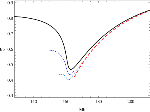
This parameter varies from for GeV to for GeV or GeV (see Figure 4), and grows monotonically towards the asymptotic value in the limit. Near or below threshold, the values of decrease in the presence of a cut.
The function , with , has only two local maxima: a broad peak at (where ), and a narrow peak at (where ). The highest maximum is the one at (0,0) for , and at for (this corresponds to GeV if there is no cut). In between these peaks there is a saddle point at . There are two minima (where ) at and , as shown in Figure 5.

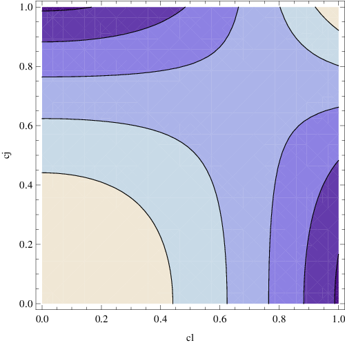
A cut that preserves as much as possible of the signal for a given reduction of the allowed region must include the broad peak, so that it can be parametrized as
| (3.34) |
where is a parameter describing how large is along the cut. For the broad peak is included up to the height of the saddle point; for the whole broad peak is cut. The region of integration corresponding to this cut is
| (3.35) |
For , the sharper peak at is high enough to warrant an additional cut around it:
| (3.36) |
where Eq. (3.34) has been used again. Integrating over and we find
| (3.37) |
Let us now turn to the case , which implies that the last term in Eq. (3.27) does not vanish. This term is induced by the interference between the longitudinal and transverse polarizations. The Higgs decay width is now as in Eq. (3.37) with replaced by , where
| (3.38) |
This last term contributes mostly near the saddle point of the , so that the contour lines change their shape, as illustrated in Figure 6. This effect is most notable near the threshold. If a standard Higgs boson with a mass not far from will be discovered, then the effects of interference should be observed through the measurement of the differential decay width as a function of and for different cuts.


4 Conclusions and outlook
The semileptonic Higgs decays and , after a mass constraint on the leptonic is imposed, resemble the golden mode in that they are fully reconstructible. The branching fractions for these modes are enhanced compared to the golden mode by a huge factor, ranging between 130 above the threshold and approximately 3000 near the threshold.
We have shown that the fully differential width for the semileptonic decays has a relatively simple dependence on the kinematic variables [see Eq. (2.13)], and that almost all features of the decay can be exhibited analytically, even with imposition of cuts on the relevant variables. In the Higgs rest frame, the decay width depends on 5 kinematic variables. Treating the leptonic in the narrow width approximation fixes the invariant mass of the system. Two other variables may be taken to be the dijet invariant mass, and the azimuthal angle of the charged lepton with respect to the dijet plane. The remaining two variables are polar angles defined in the rest frames of the dijet system, and of the system respectively. We have shown that there are interesting correlations between these polar angles, especially for Higgs masses away from the threshold (see Figure 5).
The relative neglect of these semileptonic Higgs channels in the literature, and the absence of Tevatron results for them, can be traced to the large background contributions from Standard Model processes with a leptonic , especially diboson production and inclusive production. To overcome this difficulty, it is necessary to utilize all of the distinguishing features of the signal process. The description of the fully differential Higgs decay presented here can be supplemented by the fact that the Higgs peak is reconstructed in these semileptonic decays, as well as by kinematic differences between Higgs production and the backgrounds. In combination, this allows one to design multi-dimensional cuts that may separate efficiently the signal from the background. Because the signal involves jets, it is not sufficient to study the background at the parton level; a theoretical comparison of the differential signal and backgrounds involving showering effects will be presented in an upcoming publication [14].
At the Tevatron, we expect the semileptonic channels for Higgs decay to provide a significant improvement in the overall sensitivity of the Higgs search, for a large fraction of the relevant Higgs mass range. At the LHC, the semileptonic channels should also be regarded as promising discovery channels over a broad mass range. This should include also the semileptonic Higgs decay , which can be analyzed in the same way as the semileptonic , trading a higher rate for a cleaner final state. Furthermore, these semileptonic channels can be used to supplement the fully leptonic golden mode in the characterization of a putative Higgs signal, extending the program developed in [18].
All our analytic expressions for the differential decay width and various cuts have been derived here at tree level. It turns out that the higher order effects on the shapes of the differential distributions are small, on the order of 5% [19]. Thus the analytic tree level analysis outlined here contains all of the decay information relevant to a Higgs discovery search or an initial characterization of a Higgs signal.
Acknowledgments.—We would like to thank Alvaro De Rujula, Estia Eichten, Patrick Fox, Tao Han, Robert Harr, Maurizio Pierini, Chris Rogan, Maria Spiropulu, Zack Sullivan, and especially Jan Winter for stimulating discussions. Fermilab is operated by Fermi Research Alliance, LLC, under Contract DE-AC02-07CH11359 with the United States Department of Energy.
References
- [1] For a review, see A. Djouadi, “The Anatomy of electro-weak symmetry breaking. I: The Higgs boson in the standard model,” Phys. Rept. 457, 1 (2008) [arXiv:hep-ph/0503172].
- [2] C. Amsler et al. [Particle Data Group], “Review of particle physics,” Phys. Lett. B 667, 1 (2008).
- [3] TEVNPH Working Group, for the CDF and D0 Collaborations, “Combined CDF and D0 Upper Limits on Standard Model Higgs-Boson Production with 2.1 - 5.4 fb-1 of Data,” arXiv:0911.3930 [hep-ex].
- [4] T. Han and R. J. Zhang, “Extending the Higgs boson reach at upgraded Tevatron,” Phys. Rev. Lett. 82, 25 (1999) [arXiv:hep-ph/9807424].
- [5] T. Han, A. S. Turcot and R. J. Zhang, “Exploiting decays at the upgraded Fermilab Tevatron,” Phys. Rev. D 59, 093001 (1999) [arXiv:hep-ph/9812275].
- [6] M. S. Carena et al. [Higgs Working Group Collaboration], “Report of the Tevatron Higgs working group,” arXiv:hep-ph/0010338.
- [7]
W. J. Stirling, R. Kleiss and S. D. Ellis,
“ pair production in high-energy hadronic collisions: signal versus
background,”
Phys. Lett. B 163, 261 (1985).
J. F. Gunion, P. Kalyniak, M. Soldate and P. Galison, “Hunting for the intermediate mass Higgs boson in a hadron collider,” Phys. Rev. Lett. 54, 1226 (1985).
For a review, see R. N. Cahn, “ The Higgs Boson,” Rept. Prog. Phys. 52, 389 (1989). - [8] J. F. Gunion and M. Soldate, “Overcoming a critical background to Higgs detection,” Phys. Rev. D 34, 826 (1986).
- [9] G. Aad et al. [The ATLAS Collaboration], “Expected Performance of the ATLAS Experiment - Detector, Trigger and Physics,” arXiv:0901.0512 [hep-ex].
- [10] G. L. Bayatian et al. [CMS Collaboration], “CMS technical design report, volume II: Physics performance,” J. Phys. G 34, 995 (2007).
- [11]
The D0 Collaboration,
“Search for Higgs boson production in dilepton plus missing transverse
energy final states with 5.4 fb-1 of collisions
at TeV”, D0 note 6006-CONF, November 2009.
The CDF Collaboration, “Search for production at CDF using 4.8 fb-1 of data”, CDF note 9887, August 2009. - [12] K. Iordanidis and D. Zeppenfeld, “Searching for a heavy Higgs boson via the mode at the LHC,” Phys. Rev. D 57, 3072 (1998) [arXiv:hep-ph/9709506].
- [13] B. Mellado, W. Quayle and S. L. Wu, “Feasibility of searches for a Higgs boson using +MET and high jets at the Tevatron,” Phys. Rev. D 76, 093007 (2007) [arXiv:0708.2507 [hep-ph]].
- [14] J. Winter, et al, “Semileptonic Higgs decays at the Tevatron”, to appear.
- [15] V. D. Barger, G. Bhattacharya, T. Han and B. A. Kniehl, “Intermediate mass Higgs boson at hadron supercolliders,” Phys. Rev. D 43, 779 (1991).
- [16] V. D. Barger, K. m. Cheung, A. Djouadi, B. A. Kniehl and P. M. Zerwas, “Higgs bosons: Intermediate mass range at e+ e- colliders,” Phys. Rev. D 49, 79 (1994) [arXiv:hep-ph/9306270].
- [17] C. P. Buszello, I. Fleck, P. Marquard and J. J. van der Bij, “Prospective analysis of spin- and CP-sensitive variables in at the LHC”, Eur. Phys. J. C 32, 209 (2004) [arXiv:hep-ph/0212396].
- [18] A. De Rujula, J. Lykken, M. Pierini, C. Rogan and M. Spiropulu, “Higgs Imposters at the LHC”, to appear.
- [19] A. Bredenstein, A. Denner, S. Dittmaier and M. M. Weber, “Radiative corrections to the semileptonic and hadronic Higgs-boson decays fermions,” JHEP 0702, 080 (2007) [arXiv:hep-ph/0611234].