跳到论文正文
W Papers独立论文阅读器 arXiv:0912.3449 论文正文 计算阅读时间 · 0%
引用这篇论文根据当前论文元数据生成,正式投稿前建议核对。


License: arXiv.org perpetual non-exclusive license
arXiv:0912.3449v2 [astro-ph.EP] 22 Feb 2010

Galactic tide and secular orbital evolution

P. Pástor    J. Klačka    L. Kómar Affiliation: P. Pástor Affiliation: J. Klačka Affiliation: Department of Astronomy, Physics of the Earth, and Meteorology,
Faculty of Mathematics, Physics and Informatics,
Comenius University, Mlynská dolina, 842 48 Bratislava, Slovak Republic
E-mail: {pavol.pastor,klacka,komar}@fmph.uniba.sk
Abstract

Equation of motion for the galactic tide is treated for the case of a comet situated in the Oort cloud of comets. We take into account that galactic potential and mass density depend on a distance from the galactic equator and on a distance from the rotational axis of the Galaxy. Secular evolution of orbital elements is presented. New terms generated by the Sun’s oscillation about the galactic plane are considered. The inclusion of the new terms into the equation of motion of the comet leads to orbital evolution which may be significantly different from the conventional approach. The usage of the secular time derivatives is limited to the cases when orbital period of the comet is much less than i) the period of oscillations of the Sun around the galactic equator, and, ii) the orbital period of the motion of the Sun around the galactic center.

Keywords: 
Galaxy Oort cloud of comets Orbital evolution

1 Introduction

Global galactic gravitational field influences motion of a comet in the Oort cloud in the form of the galactic tide. The motion of the comet with respect to the Sun is important in better understanding of the Oort cloud. This paper presents equations for secular evolution of orbital elements for the comet under the gravity of the Sun and the galactic tide. We consider equation of motion derived in Klačka (2009a). Results of our paper reduce to the results obtained by Klačka and Gajdošík (1999) and Fouchard et al. (2005) when several physical terms are ignored. The results are compared with detailed numerical solution of the equation of motion given by Kómar et al. (2009).

2 Equation of motion

We are interested in motion of a comet with respect to the Sun. The comet is in the Oort cloud and we want to describe the cometary evolution in terms of secular evolution of comet’s orbital elements.

The Sun is moving at a distance R0R_{0} == 8 kpc from the center of the Galaxy. Currently, the Sun is situated 30 pc above the galactic equatorial plane (Z0Z_{0} == 30 pc). Besides rotational motion with the speed (AA −- BB) ×\times R0R_{0} (where AA and BB are Oort constants) the Sun is moving with the speed 7.3 km/s in the direction normal to the galactic plane. Positional vector of the comet with respect to the Sun is r→\vec{r} == (ξ\xi, η\eta, ζ\zeta). Equation of motion is taken in the form

d2​ξd​t2\displaystyle\frac{d^{2}\xi}{dt^{2}} =\displaystyle= −G​M⊙r3​ξ+(A−B)​[A+B+2​A​cos⁡(2​ω0​t)]​ξ\displaystyle-~\frac{GM_{\odot}}{r^{3}}~\xi~+~(A-B)\left[A+B+2A\cos\left(2~\omega_{0}t\right)\right]~\xi
−2​A​(A−B)​sin⁡(2​ω0​t)​η\displaystyle-~2A(A-B)\sin\left(2~\omega_{0}t\right)~\eta
+2​(A−B)2​(Γ1−Γ2​Z02)​R0​Z0​cos⁡(ω0​t)​ζ,\displaystyle+~2(A-B)^{2}~(\Gamma_{1}-\Gamma_{2}Z_{0}^{2})~R_{0}~Z_{0}~\cos\left(\omega_{0}t\right)~\zeta~,
d2​ηd​t2\displaystyle\frac{d^{2}\eta}{dt^{2}} =\displaystyle= −G​M⊙r3​η−2​A​(A−B)​sin⁡(2​ω0​t)​ξ\displaystyle-~\frac{GM_{\odot}}{r^{3}}~\eta~-~2A(A-B)\sin\left(2~\omega_{0}t\right)~\xi
+(A−B)​[A+B−2​A​cos⁡(2​ω0​t)]​η\displaystyle+~(A-B)\left[A+B-2A\cos\left(2~\omega_{0}t\right)\right]~\eta
−2​(A−B)2​(Γ1−Γ2​Z02)​R0​Z0​sin⁡(ω0​t)​ζ,\displaystyle-~2(A-B)^{2}~(\Gamma_{1}-\Gamma_{2}Z_{0}^{2})~R_{0}~Z_{0}~\sin\left(\omega_{0}t\right)~\zeta~,
d2​ζd​t2\displaystyle\frac{d^{2}\zeta}{dt^{2}} =\displaystyle= −G​M⊙r3​ζ−[4​π​G​ϱ+2​(A2−B2)]​ζ\displaystyle-~\frac{GM_{\odot}}{r^{3}}~\zeta~-~\left[4~\pi~G~\varrho~+~2\left(A^{2}~-~B^{2}\right)\right]~\zeta
−4​π​G​ϱ′​Z0​[cos⁡(ω0​t)​ξ−sin⁡(ω0​t)​η],\displaystyle-~4~\pi~G~\varrho^{\prime}~Z_{0}\left[\cos\left(\omega_{0}t\right)~\xi~-~\sin\left(\omega_{0}t\right)~\eta\right]~,
d2​Z0d​t2\displaystyle\frac{d^{2}Z_{0}}{dt^{2}} =\displaystyle= −[4​π​G​ϱ+2​(A2−B2)]​Z0,\displaystyle-~\left[4~\pi~G~\varrho~+~2\left(A^{2}~-~B^{2}\right)\right]~Z_{0}~,
r\displaystyle r =\displaystyle= ξ2+η2+ζ2,\displaystyle\sqrt{\xi^{2}~+~\eta^{2}~+~\zeta^{2}}~,
ω0\displaystyle\omega_{0} =\displaystyle= A−B,\displaystyle A~-~B~, (1)

where GG is the gravitational constant, M⊙M_{\odot} is the mass of the Sun and

A\displaystyle A =\displaystyle= 14.2​km​s−1​kpc−1,\displaystyle 14.2~\mbox{km}~\mbox{s}^{-1}~\mbox{kpc}^{-1}~,
B\displaystyle B =\displaystyle= −12.4​km​s−1​kpc−1,\displaystyle-12.4~\mbox{km}~\mbox{s}^{-1}~\mbox{kpc}^{-1}~,
Γ1\displaystyle\Gamma_{1} =\displaystyle= 0.124​kpc−2,\displaystyle 0.124~\mbox{kpc}^{-2}~,
Γ2\displaystyle\Gamma_{2} =\displaystyle= 1.586​kpc−4,\displaystyle 1.586~\mbox{kpc}^{-4}~,
ϱ\displaystyle\varrho =\displaystyle= 0.130​M⊙​pc−3,\displaystyle 0.130~\mbox{M}_{\odot}~\mbox{pc}^{-3}~,
ϱ′\displaystyle\varrho^{\prime} =\displaystyle= −0.037​M⊙​pc−3​kpc−1,\displaystyle-0.037~\mbox{M}_{\odot}~\mbox{pc}^{-3}~\mbox{kpc}^{-1}~, (2)

see Eqs. (26)-(27) in Klačka (2009a). If one wants to use other values of the Oort constants AA and BB, he can use Eqs. (22) in Klačka (2009a):

ϱ\displaystyle\varrho =\displaystyle= ϱd​i​s​k+ϱh​a​l​o,\displaystyle\varrho_{disk}~+~\varrho_{halo}~,
ϱd​i​s​k\displaystyle\varrho_{disk} =\displaystyle= 0.126​M⊙​pc−3,\displaystyle 0.126~\mbox{M}_{\odot}~\mbox{pc}^{-3}~,
ϱh​a​l​o\displaystyle\varrho_{halo} =\displaystyle= (4​π​G)−1​[X⁡(G​a​l​a​x​y)+X⁡(d​i​s​k)+X⁡(b​u​l​g​e)],\displaystyle(4\pi G)^{-1}[X(Galaxy)+X(disk)+X(bulge)]~,
X⁡(G​a​l​a​x​y)\displaystyle X(Galaxy) ≡\displaystyle\equiv −(A−B)×(A+3B)\displaystyle-(A-B)\times(A+3B)
X⁡(d​i​s​k)\displaystyle X(disk) =\displaystyle= −396.90​km2​s−2​kpc−2,\displaystyle-~396.90~\mbox{km}^{2}~\mbox{s}^{-2}~\mbox{kpc}^{-2}~,
X⁡(b​u​l​g​e)\displaystyle X(bulge) =\displaystyle= −0.65​km2​s−2​kpc−2,\displaystyle-~0.65~\mbox{km}^{2}~\mbox{s}^{-2}~\mbox{kpc}^{-2}~, (3)

The value X⁡(G​a​l​a​x​y)X(Galaxy) == 611.800 km2 s-2 kpc-2 holds for AA == 14.2  km  s-1  kpc-1 and BB == −- 12.4 km  s-1  kpc-1. Eqs. (22) of Klačka (2009a) can be used.

Refer to caption
Refer to caption
Refer to caption
Refer to caption
Refer to caption
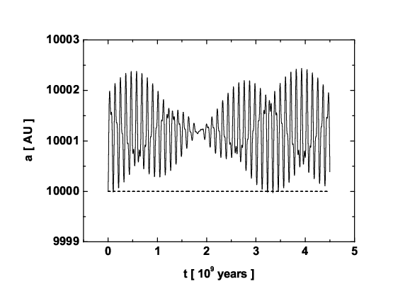
Figure 1: Two orbital evolutions of a comet with initial semi-major axis 10000 AU in the Oort cloud under the influence of galactic tide. Evolutions are obtained from numerical solution of system of differential equations given by Eqs. (13)-(17) with the new terms (solid line) and without new terms (dashed line).
Refer to caption
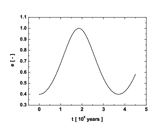
Figure 2: Time evolution of eccentricity when initial eccentricity is close to zero.

3 Secular changes of orbital elements

Perturbation equations of celestial mechanics yield for osculating orbital elements (aa – semi-major axis; ee – eccentricity; ii – inclination (of the orbital plane to the reference plane – galactic equatorial plane); Ω\Omega – longitude of the ascending node; ω\omega – argument of perihelion; Θ\Theta is the position angle of the particle on the orbit, when measured from the ascending node in the direction of the particle’s motion, Θ=ω+f\Theta=\omega+f):

d​ad​t\displaystyle\frac{da}{dt} =\displaystyle= 2​a1−e2​pμ​{FR​e​sin⁡f+FT​(1+e​cos⁡f)},\displaystyle\frac{2~a}{1~-~e^{2}}~\sqrt{\frac{p}{\mu}}~\left\{F_{R}~e~\sin f+F_{T}\left(1~+~e~\cos f\right)\right\}~,
d​ed​t\displaystyle\frac{de}{dt} =\displaystyle= pμ​{FR​sin⁡f+FT​[cos⁡f+e+cos⁡f1+e​cos⁡f]},\displaystyle\sqrt{\frac{p}{\mu}}~\left\{F_{R}~\sin f+F_{T}\left[\cos f~+~\frac{e+\cos f}{1+e\cos f}\right]\right\}~,
d​id​t\displaystyle\frac{di}{dt} =\displaystyle= rμ​p​FN​cos⁡Θ,\displaystyle\frac{r}{\sqrt{\mu~p}}~F_{N}~\cos\Theta~,
d​Ωd​t\displaystyle\frac{d\Omega}{dt} =\displaystyle= rμ​p​FN​sin⁡Θsin⁡i,\displaystyle\frac{r}{\sqrt{\mu~p}}~F_{N}~\frac{\sin\Theta}{\sin i}~,
d​ωd​t\displaystyle\frac{d\omega}{dt} =\displaystyle= −1e​pμ​{FR​cos⁡f−FT​2+e​cos⁡f1+e​cos⁡f​sin⁡f}\displaystyle-~\frac{1}{e}~\sqrt{\frac{p}{\mu}}~\left\{F_{R}\cos f-F_{T}~\frac{2+e\cos f}{1+e\cos f}~\sin f\right\}
−rμ​p​FN​sin⁡Θsin⁡i​cos⁡i,\displaystyle-~\frac{r}{\sqrt{\mu~p}}~F_{N}~\frac{\sin\Theta}{\sin i}~\cos i~,
d​Θd​t\displaystyle\frac{d\Theta}{dt} =\displaystyle= μ​pr2−rμ​p​FN​sin⁡Θsin⁡i​cos⁡i,\displaystyle\frac{\sqrt{\mu~p}}{r^{2}}~-~\frac{r}{\sqrt{\mu~p}}~F_{N}~\frac{\sin\Theta}{\sin i}~\cos i~,
r\displaystyle r =\displaystyle= p/(1+e​cos⁡f),\displaystyle p/(1+e\cos f)~,
p\displaystyle p =\displaystyle= a⁡(1−e2),\displaystyle a~(1-e^{2})~,
μ\displaystyle\mu ≡\displaystyle\equiv G​M⊙,\displaystyle GM_{\odot}~, (4)

where FRF_{R}, FTF_{T} and FNF_{N} are radial, transversal and normal components of the disturbing acceleration. We use −μe→R/r2-~\mu~\vec{e}_{R}~/~r^{2} as a central acceleration determining osculating orbital elements if we want to take a time average (TT is time interval between passages through two following pericenters) in an analytical way

⟨g⟩\displaystyle\langle g\rangle ≡\displaystyle\equiv 1T​∫0Tg⁡(t)​𝑑t=μa3/2​12​π​∫02​πg⁡(f)​(d​fd​t)−1​𝑑f\displaystyle\frac{1}{T}\int_{0}^{T}g(t)dt=\frac{\sqrt{\mu}}{a^{3/2}}~\frac{1}{2\pi}\int_{0}^{2\pi}g(f)\left(\frac{df}{dt}\right)^{-1}df (5)
=\displaystyle= μa3/2​12​π​∫02​πg⁡(f)​r2μ​p​𝑑f\displaystyle\frac{\sqrt{\mu}}{a^{3/2}}~\frac{1}{2\pi}\int_{0}^{2\pi}g(f)~\frac{r^{2}}{\sqrt{\mu~p}}~df
=\displaystyle= 1a2​1−e2​12​π​∫02​πg⁡(f)​r2​𝑑f,\displaystyle\frac{1}{a^{2}~\sqrt{1-e^{2}}}~\frac{1}{2\pi}~\int_{0}^{2\pi}~g(f)~r^{2}~df~,

assuming non-pseudo-circular orbits and the fact that orbital elements exhibit only small changes during the time interval TT; the second and the third Kepler’s laws were used: r2​d​f/d​t=μ​pr^{2}~df/dt=\sqrt{\mu p} – conservation of angular momentum, a3/T2=μ/(4​π2)a^{3}/T^{2}=\mu/(4\pi^{2}).

Rewriting Eq. (1) to the form

d2​ξd​t2\displaystyle\frac{d^{2}\xi}{dt^{2}} =\displaystyle= −G​M⊙r3​ξ+Fx,\displaystyle-~\frac{GM_{\odot}}{r^{3}}~\xi~+~F_{x}~,
d2​ηd​t2\displaystyle\frac{d^{2}\eta}{dt^{2}} =\displaystyle= −G​M⊙r3​η+Fy,\displaystyle-~\frac{GM_{\odot}}{r^{3}}~\eta~+~F_{y}~,
d2​ζd​t2\displaystyle\frac{d^{2}\zeta}{dt^{2}} =\displaystyle= −G​M⊙r3​ζ+Fz,\displaystyle-~\frac{GM_{\odot}}{r^{3}}~\zeta~+~F_{z}~,
r\displaystyle r =\displaystyle= ξ2+η2+ζ2,\displaystyle\sqrt{\xi^{2}~+~\eta^{2}~+~\zeta^{2}}~,
Fx\displaystyle F_{x} =\displaystyle= (A−B)​[A+B+2​A​cos⁡(2​ω0​t)]​ξ−2​A​(A−B)​sin⁡(2​ω0​t)​η\displaystyle(A-B)\left[A+B+2A\cos\left(2~\omega_{0}t\right)\right]~\xi~-~2A(A-B)\sin\left(2~\omega_{0}t\right)~\eta
+2​(A−B)2​(Γ1−Γ2​Z02)​R0​Z0​cos⁡(ω0​t)​ζ,\displaystyle+~2(A-B)^{2}~(\Gamma_{1}-\Gamma_{2}Z_{0}^{2})~R_{0}~Z_{0}~\cos\left(\omega_{0}t\right)~\zeta~,
Fy\displaystyle F_{y} =\displaystyle= −2​A​(A−B)​sin⁡(2​ω0​t)​ξ+(A−B)​[A+B−2​A​cos⁡(2​ω0​t)]​η\displaystyle-~2A(A-B)\sin\left(2~\omega_{0}t\right)~\xi~+~(A-B)\left[A+B-2A\cos\left(2~\omega_{0}t\right)\right]~\eta
−2​(A−B)2​(Γ1−Γ2​Z02)​R0​Z0​sin⁡(ω0​t)​ζ,\displaystyle-~2(A-B)^{2}~(\Gamma_{1}-\Gamma_{2}Z_{0}^{2})~R_{0}~Z_{0}~\sin\left(\omega_{0}t\right)~\zeta~,
Fz\displaystyle F_{z} =\displaystyle= −ωz2​ζ−4​π​G​ϱ′​Z0​[cos⁡(ω0​t)​ξ−sin⁡(ω0​t)​η],\displaystyle-~\omega_{z}^{2}~\zeta~-~4~\pi~G~\varrho^{\prime}~Z_{0}\left[\cos\left(\omega_{0}t\right)~\xi~-~\sin\left(\omega_{0}t\right)~\eta\right]~,
Z0\displaystyle Z_{0} =\displaystyle= K​sin⁡(ωz​t+φ0),\displaystyle K~\sin(\omega_{z}~t+\varphi_{0})~,
Z0​(t=t0)\displaystyle Z_{0}(t=t_{0}) =\displaystyle= 30​pc=6.188×10⁶​AU,\displaystyle 30~\mbox{pc}=6.188\times 10^{6}~\mbox{AU}~,
Z0˙​(t=t0)\displaystyle\dot{Z_{0}}(t=t_{0}) =\displaystyle= 7.3​km​s−1=1.540​AU​yr−1,\displaystyle 7.3~\mbox{km}~\mbox{s}^{-1}=1.540~\mbox{AU}~\mbox{yr}^{-1}~,
ωz\displaystyle\omega_{z} =\displaystyle= 4​π​G​ϱ+2​(A2−B2),\displaystyle\sqrt{4~\pi~G~\varrho~+~2\left(A^{2}~-~B^{2}\right)}~,
ω0\displaystyle\omega_{0} =\displaystyle= A−B,\displaystyle A~-~B~, (6)

where t0t_{0} denotes the current time moment and φ0\varphi_{0} the initial phase, we can find the required components FRF_{R}, FTF_{T} and FNF_{N} of the disturbing acceleration:

FR\displaystyle F_{R} =\displaystyle= F→⋅e→R≡Fx​eR​x+Fy​eR​y+Fz​eR​z,\displaystyle\vec{F}\cdot\vec{e}_{R}\equiv F_{x}~e_{R~x}~+~F_{y}~e_{R~y}~+~F_{z}~e_{R~z}~,
FT\displaystyle F_{T} =\displaystyle= F→⋅e→T≡Fx​eT​x+Fy​eT​y+Fz​eT​z,\displaystyle\vec{F}\cdot\vec{e}_{T}\equiv F_{x}~e_{T~x}~+~F_{y}~e_{T~y}~+~F_{z}~e_{T~z}~,
FN\displaystyle F_{N} =\displaystyle= F→⋅e→N≡Fx​eN​x+Fy​eN​y+Fz​eN​z,\displaystyle\vec{F}\cdot\vec{e}_{N}\equiv F_{x}~e_{N~x}~+~F_{y}~e_{N~y}~+~F_{z}~e_{N~z}~,
e→R\displaystyle\vec{e}_{R} =\displaystyle= (cos⁡Ω​cos⁡Θ−sin⁡Ω​sin⁡Θ​cos⁡iCLOSE,\displaystyle(\cos\Omega~\cos\Theta~-~\sin\Omega~\sin\Theta~\cos i,
OPENsin⁡Ω​cos⁡Θ+cos⁡Ω​sin⁡Θ​cos⁡i,sin⁡Θ​sin⁡i),\displaystyle\sin\Omega~\cos\Theta~+~\cos\Omega~\sin\Theta~\cos i,\sin\Theta~\sin i)~,
e→T\displaystyle\vec{e}_{T} =\displaystyle= (−cos⁡Ω​sin⁡Θ−sin⁡Ω​cos⁡Θ​cos⁡iCLOSE,\displaystyle(-~\cos\Omega~\sin\Theta~-~\sin\Omega~\cos\Theta~\cos i,
OPEN−sin⁡Ω​sin⁡Θ+cos⁡Ω​cos⁡Θ​cos⁡i,cos⁡Θ​sin⁡i),\displaystyle-~\sin\Omega~\sin\Theta~+~\cos\Omega~\cos\Theta~\cos i,\cos\Theta~\sin i)~,
e→N\displaystyle\vec{e}_{N} =\displaystyle= (sin⁡Ω​sin⁡i,−cos⁡Ω​sin⁡i,cos⁡i).\displaystyle(\sin\Omega~\sin i,-\cos\Omega~\sin i,\cos i)~. (7)

Inserting Eqs. (6) into Eqs. (7):

FR\displaystyle F_{R} =\displaystyle= {(A−B)[A+B+2Acos(2ω0t)]r(cosΩcosΘ−sinΩsinΘcosi)\displaystyle\bigl\{(A-B)\left[A+B+2A\cos\left(2~\omega_{0}t\right)\right]~r~(\cos\Omega~\cos\Theta~-~\sin\Omega~\sin\Theta~\cos i) (8)
−2​A​(A−B)​sin⁡(2​ω0​t)​r​(sin⁡Ω​cos⁡Θ+cos⁡Ω​sin⁡Θ​cos⁡i)\displaystyle-~2A(A-B)\sin\left(2~\omega_{0}t\right)~r~(\sin\Omega~\cos\Theta~+~\cos\Omega~\sin\Theta~\cos i)
+2(A−B)2(Γ1−Γ2Z02)R0Z0cos(ω0t)rsinΘsini}×\displaystyle+~2(A-B)^{2}~(\Gamma_{1}-\Gamma_{2}Z_{0}^{2})~R_{0}~Z_{0}~\cos\left(\omega_{0}t\right)~r~\sin\Theta~\sin i\bigr\}~\times
×(cos⁡Ω​cos⁡Θ−sin⁡Ω​sin⁡Θ​cos⁡i)\displaystyle\times~(\cos\Omega~\cos\Theta~-~\sin\Omega~\sin\Theta~\cos i)
+{−2A(A−B)sin(2ω0t)r(cosΩcosΘ−sinΩsinΘcosi)\displaystyle+~\bigl\{-~2A(A-B)\sin\left(2~\omega_{0}t\right)~r~(\cos\Omega~\cos\Theta~-~\sin\Omega~\sin\Theta~\cos i)
+(A−B)​[A+B−2​A​cos⁡(2​ω0​t)]​r​(sin⁡Ω​cos⁡Θ+cos⁡Ω​sin⁡Θ​cos⁡i)\displaystyle+~(A-B)\left[A+B-2A\cos\left(2~\omega_{0}t\right)\right]~r~(\sin\Omega~\cos\Theta~+~\cos\Omega~\sin\Theta~\cos i)
−2(A−B)2(Γ1−Γ2Z02)R0Z0sin(ω0t)rsinΘsini}×\displaystyle-~2(A-B)^{2}~(\Gamma_{1}-\Gamma_{2}Z_{0}^{2})~R_{0}~Z_{0}~\sin\left(\omega_{0}t\right)~r~\sin\Theta~\sin i\bigr\}~\times
×(sin⁡Ω​cos⁡Θ+cos⁡Ω​sin⁡Θ​cos⁡i)\displaystyle\times~(\sin\Omega~\cos\Theta~+~\cos\Omega~\sin\Theta~\cos i)
+{−ωz2rsinΘsini\displaystyle+~\bigl\{-~\omega_{z}^{2}~r~\sin\Theta~\sin i
−4πGϱ′Z0r[cos(ω0t)(cosΩcosΘ−sinΩsinΘcosi)\displaystyle-~4~\pi~G~\varrho^{\prime}~Z_{0}~r~\bigl[\cos\left(\omega_{0}t\right)~(\cos\Omega~\cos\Theta~-~\sin\Omega~\sin\Theta~\cos i)
−sin(ω0t)(sinΩcosΘ+cosΩsinΘcosi)]}×sinΘsini,\displaystyle-~\sin\left(\omega_{0}t\right)~(\sin\Omega~\cos\Theta~+~\cos\Omega~\sin\Theta~\cos i)\bigr]\bigr\}\times~\sin\Theta~\sin i~,
FT\displaystyle F_{T} =\displaystyle= {(A−B)[A+B+2Acos(2ω0t)]r(cosΩcosΘ−sinΩsinΘcosi)\displaystyle\bigl\{(A-B)\left[A+B+2A\cos\left(2~\omega_{0}t\right)\right]~r~(\cos\Omega~\cos\Theta~-~\sin\Omega~\sin\Theta~\cos i) (9)
−2​A​(A−B)​sin⁡(2​ω0​t)​r​(sin⁡Ω​cos⁡Θ+cos⁡Ω​sin⁡Θ​cos⁡i)\displaystyle-~2A(A-B)\sin\left(2~\omega_{0}t\right)~r~(\sin\Omega~\cos\Theta~+~\cos\Omega~\sin\Theta~\cos i)
+2(A−B)2(Γ1−Γ2Z02)R0Z0cos(ω0t)rsinΘsini}×\displaystyle+~2(A-B)^{2}~(\Gamma_{1}-\Gamma_{2}Z_{0}^{2})~R_{0}~Z_{0}~\cos\left(\omega_{0}t\right)~r~\sin\Theta~\sin i\bigr\}~\times
×(−cos⁡Ω​sin⁡Θ−sin⁡Ω​cos⁡Θ​cos⁡i)\displaystyle\times~(-~\cos\Omega~\sin\Theta~-~\sin\Omega~\cos\Theta~\cos i)
+{−2A(A−B)sin(2ω0t)r(cosΩcosΘ−sinΩsinΘcosi)\displaystyle+~\bigl\{-~2A(A-B)\sin\left(2~\omega_{0}t\right)~r~(\cos\Omega~\cos\Theta~-~\sin\Omega~\sin\Theta~\cos i)
+(A−B)​[A+B−2​A​cos⁡(2​ω0​t)]​r​(sin⁡Ω​cos⁡Θ+cos⁡Ω​sin⁡Θ​cos⁡i)\displaystyle+~(A-B)\left[A+B-2A\cos\left(2~\omega_{0}t\right)\right]~r~(\sin\Omega~\cos\Theta~+~\cos\Omega~\sin\Theta~\cos i)
−2(A−B)2(Γ1−Γ2Z02)R0Z0sin(ω0t)rsinΘsini}×\displaystyle-~2(A-B)^{2}~(\Gamma_{1}-\Gamma_{2}Z_{0}^{2})~R_{0}~Z_{0}~\sin\left(\omega_{0}t\right)~r~\sin\Theta~\sin i\bigr\}~\times
×(−sin⁡Ω​sin⁡Θ+cos⁡Ω​cos⁡Θ​cos⁡i)\displaystyle\times~(-~\sin\Omega~\sin\Theta~+~\cos\Omega~\cos\Theta~\cos i)
+{−ωz2rsinΘsini\displaystyle+~\bigl\{-~\omega_{z}^{2}~r~\sin\Theta~\sin i
−4πGϱ′Z0r[cos(ω0t)(cosΩcosΘ−sinΩsinΘcosi)\displaystyle-~4~\pi~G~\varrho^{\prime}~Z_{0}~r~\bigl[\cos\left(\omega_{0}t\right)~(\cos\Omega~\cos\Theta~-~\sin\Omega~\sin\Theta~\cos i)
−sin(ω0t)(sinΩcosΘ+cosΩsinΘcosi)]}×cosΘsini,\displaystyle-~\sin\left(\omega_{0}t\right)~(\sin\Omega~\cos\Theta~+~\cos\Omega~\sin\Theta~\cos i)\bigr]\bigr\}\times~\cos\Theta~\sin i~,
FN\displaystyle F_{N} =\displaystyle= {(A−B)[A+B+2Acos(2ω0t)]r(cosΩcosΘ−sinΩsinΘcosi)\displaystyle\bigl\{(A-B)\left[A+B+2A\cos\left(2~\omega_{0}t\right)\right]~r~(\cos\Omega~\cos\Theta~-~\sin\Omega~\sin\Theta~\cos i) (10)
−2​A​(A−B)​sin⁡(2​ω0​t)​r​(sin⁡Ω​cos⁡Θ+cos⁡Ω​sin⁡Θ​cos⁡i)\displaystyle-~2A(A-B)\sin\left(2~\omega_{0}t\right)~r~(\sin\Omega~\cos\Theta~+~\cos\Omega~\sin\Theta~\cos i)
+2(A−B)2(Γ1−Γ2Z02)R0Z0cos(ω0t)rsinΘsini}×(sinΩsini)\displaystyle+~2(A-B)^{2}~(\Gamma_{1}-\Gamma_{2}Z_{0}^{2})~R_{0}~Z_{0}~\cos\left(\omega_{0}t\right)~r~\sin\Theta~\sin i\bigr\}~\times~(\sin\Omega~\sin i)
+{−2A(A−B)sin(2ω0t)r(cosΩcosΘ−sinΩsinΘcosi)\displaystyle+~\bigl\{-~2A(A-B)\sin\left(2~\omega_{0}t\right)~r~(\cos\Omega~\cos\Theta~-~\sin\Omega~\sin\Theta~\cos i)
+(A−B)​[A+B−2​A​cos⁡(2​ω0​t)]​r​(sin⁡Ω​cos⁡Θ+cos⁡Ω​sin⁡Θ​cos⁡i)\displaystyle+~(A-B)\left[A+B-2A\cos\left(2~\omega_{0}t\right)\right]~r~(\sin\Omega~\cos\Theta~+~\cos\Omega~\sin\Theta~\cos i)
−2(A−B)2(Γ1−Γ2Z02)R0Z0sin(ω0t)rsinΘsini}×(−cosΩsini)\displaystyle-~2(A-B)^{2}~(\Gamma_{1}-\Gamma_{2}Z_{0}^{2})~R_{0}~Z_{0}~\sin\left(\omega_{0}t\right)~r~\sin\Theta~\sin i\bigr\}~\times~(-\cos\Omega~\sin i)
+{−ωz2rsinΘsini\displaystyle+~\bigl\{-~\omega_{z}^{2}~r~\sin\Theta~\sin i
−4πGϱ′Z0r[cos(ω0t)(cosΩcosΘ−sinΩsinΘcosi)\displaystyle-~4~\pi~G~\varrho^{\prime}~Z_{0}~r~\bigl[\cos\left(\omega_{0}t\right)~(\cos\Omega~\cos\Theta~-~\sin\Omega~\sin\Theta~\cos i)
−sin(ω0t)(sinΩcosΘ+cosΩsinΘcosi)]}×cosi.\displaystyle-~\sin\left(\omega_{0}t\right)~(\sin\Omega~\cos\Theta~+~\cos\Omega~\sin\Theta~\cos i)\bigr]\bigr\}\times~\cos i~.
Refer to caption
Refer to caption
Refer to caption
Refer to caption
Refer to caption
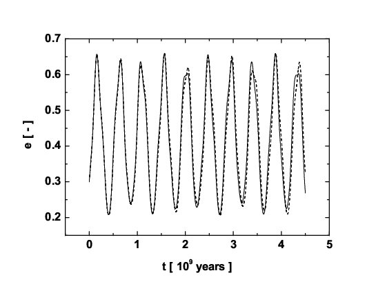
Figure 3: Comparison of two orbital evolutions of a comet with initial semi-major axis 10000 AU obtained by numerical solution of Eqs. (1) (solid line) and Eqs. (13)-(17) (dashed line). In both numerical solutions are the new terms included.

3.1 A method of averaging

Inserting Eqs. (8)-(10) into Eqs. (4) and making time averaging represented by Eq. (5), we need also the relation between the time tt and the true anomaly ff. The relation d​tdt == (r2/μ​pr^{2}/\sqrt{\mu~p}) d​fdf yields

t\displaystyle t =\displaystyle= τ+a3/2μ​{2​arctan⁡(1−e1+e​tan⁡f2)−e​1−e2​sin⁡f1+e​cos⁡f},\displaystyle\tau~+~\frac{a^{3/2}}{\sqrt{\mu}}~\left\{2~\arctan\left(\sqrt{\frac{1-e}{1+e}}~\tan\frac{f}{2}\right)~-~e~\sqrt{1-e^{2}}~\frac{\sin f}{1+e\cos f}\right\}~, (11)

if we take f⁡(t=τ)=f(t=\tau)= 0.

Another possibility is to use the Kepler’s equation t=τ+(a3/2/μ)​(E−e​sin⁡E)t=\tau+(a^{3/2}/\sqrt{\mu})(E~-~e~\sin E) [see also Eq. (11) together with tan⁡(E/2)\tan(E/2) == (1−e)/(1+e)\sqrt{(1-e)/(1+e)} tan⁡(f/2)\tan(f/2)]. Then, instead of Eq. (5), we obtain

⟨g⟩\displaystyle\langle g\rangle =\displaystyle= 12​π​∫02​πg⁡(E)​(1−e​cos⁡E)​𝑑E,\displaystyle\frac{1}{2\pi}~\int_{0}^{2\pi}~g(E)~(1~-~e~\cos E)~dE~,
sin⁡f\displaystyle\sin f =\displaystyle= a​1−e2r​sin⁡E,\displaystyle\frac{a~\sqrt{1~-~e^{2}}}{r}~\sin E~,
cos⁡f\displaystyle\cos f =\displaystyle= ar​(cos⁡E−e),\displaystyle\frac{a}{r}~\left(\cos E~-~e\right)~,
r\displaystyle r =\displaystyle= a⁡(1−e​cos⁡E),\displaystyle a~(1~-~e~\cos E)~,
t\displaystyle t =\displaystyle= τ+(a3/2/μ)​(E−e​sin⁡E).\displaystyle\tau+(a^{3/2}/\sqrt{\mu})(E~-~e~\sin E)~. (12)
Refer to caption
Refer to caption
Refer to caption
Refer to caption
Refer to caption
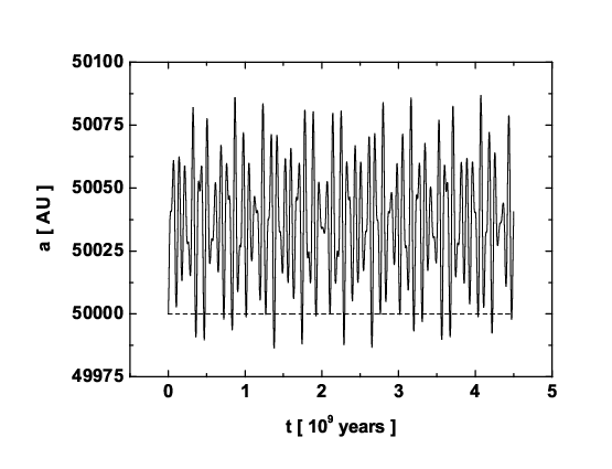
Figure 4: Comparison of two orbital evolutions of a comet with initial semi-major axis 50000 AU obtained by numerical solution of Eqs. (1) (solid line) and Eqs. (13)-(17) (dashed line). In both numerical solutions are the new terms included.

3.2 Another method of averaging

The procedure of averaging may not take into account time evolution in ω0​t\omega_{0}t and ωz​t\omega_{z}t during one orbital period if 2​π/ω02\pi/\omega_{0} ≫\gg TT and 2​π/ωz2\pi/\omega_{z} ≫\gg TT.

The secular evolution of orbital elements (and other quantitites) can be calculated on the basis of Eqs. (4)-(5) and (8)-(10). We define Ω~\tilde{\Omega} as Ω~\tilde{\Omega} == Ω\Omega ++ ω0​t\omega_{0}t. The final result then can be summarized in the form

⟨d​ad​t⟩\displaystyle\left\langle\frac{da}{dt}\right\rangle =\displaystyle= −a2​pμ​Xa​Z0​sin⁡i​cos⁡Ω~,\displaystyle-~a^{2}~\sqrt{\frac{p}{\mu}}~X_{a}~Z_{0}~\sin i~\cos\tilde{\Omega}~,
Xa\displaystyle X_{a} =\displaystyle= 2​(A−B)2​(Γ1−Γ2​Z02)​R0+4​π​G​ϱ′,\displaystyle 2(A-B)^{2}~(\Gamma_{1}-\Gamma_{2}Z_{0}^{2})~R_{0}~+~4~\pi~G~\varrho^{\prime}~, (13)
⟨d​ed​t⟩\displaystyle\left\langle\frac{de}{dt}\right\rangle =\displaystyle= 5​a​e4pμ{4A(A−B)[cosicos2ωsin2Ω~\displaystyle\frac{5ae}{4}~\sqrt{\frac{p}{\mu}}~\bigl\{4A(A-B)~\bigl[\cos i~\cos 2\omega~\sin 2\tilde{\Omega} (14)
+sin2ω(cos2Ω~−cos2isin2Ω~)]\displaystyle+~\sin 2\omega~(\cos^{2}\tilde{\Omega}-\cos^{2}i~\sin^{2}\tilde{\Omega})\bigr]
+[4πGϱ+2(A2−B2)−(A−B)2]sin2isin2ω}\displaystyle+~\bigl[4~\pi~G~\varrho+2(A^{2}-B^{2})-(A-B)^{2}\bigr]~\sin^{2}i~\sin 2\omega\bigr\}
+5​a​e​pμ​(A−B)2​(Γ1−Γ2​Z02)​R0​Z0​sin⁡i​sin⁡ω\displaystyle+~5ae~\sqrt{\frac{p}{\mu}}~(A-B)^{2}~(\Gamma_{1}-\Gamma_{2}Z_{0}^{2})~R_{0}~Z_{0}~\sin i~\sin\omega
×(cos⁡i​cos⁡ω​sin⁡Ω~+sin⁡ω​cos⁡Ω~)\displaystyle\times~\bigl(\cos i~\cos\omega~\sin\tilde{\Omega}+\sin\omega~\cos\tilde{\Omega}\bigr)
+5​a​e2​pμ​4​π​G​ϱ′​Z0​sin⁡i​cos⁡ω\displaystyle+~\frac{5ae}{2}~\sqrt{\frac{p}{\mu}}~4~\pi~G~\varrho^{\prime}~Z_{0}~\sin i~\cos\omega
×(cos⁡ω​cos⁡Ω~−cos⁡i​sin⁡ω​sin⁡Ω~),\displaystyle\times~(\cos~\omega~\cos\tilde{\Omega}-\cos i~\sin\omega~\sin\tilde{\Omega})~,
⟨d​ωd​t⟩\displaystyle\left\langle\frac{d\omega}{dt}\right\rangle =\displaystyle= −A(A−B)pμa[5(cosisin2ωsin2Ω~\displaystyle-~A(A-B)~\sqrt{\frac{p}{\mu}}~a~\bigl[5~(\cos i~\sin 2\omega~\sin 2\tilde{\Omega} (15)
OPEN−2​cos⁡2​ω​cos2⁡Ω~)+(5​cos⁡2​ω−3)\displaystyle-~2\cos 2\omega~\cos^{2}\tilde{\Omega})+~(5\cos 2\omega-3)
×(cos2⁡Ω~+11−e2​cos2⁡i​sin2⁡Ω~)\displaystyle\times~\bigl(\cos^{2}\tilde{\Omega}+\frac{1}{1-e^{2}}~\cos^{2}i~\sin^{2}\tilde{\Omega}\bigr)
+cos⁡i1−e2​(5​e2​sin⁡2​ω​sin⁡Ω~​cos⁡Ω~CLOSE\displaystyle+~\frac{\cos i}{1-e^{2}}~\bigl(5e^{2}\sin 2\omega~\sin\tilde{\Omega}~\cos\tilde{\Omega}
−2cosisin2Ω~)]\displaystyle-~2\cos i~\sin^{2}\tilde{\Omega}\bigr)\bigr]
+a4​(1−e2)​pμ​[4​π​G​ϱ+2​(A2−B2)−(A−B)2]\displaystyle+~\frac{a}{4(1-e^{2})}~\sqrt{\frac{p}{\mu}}~\bigl[4~\pi~G~\varrho+2(A^{2}-B^{2})-(A-B)^{2}\bigr]
×[(sin2⁡i−e2)​(5​cos⁡2​ω−3)+2​cos2⁡i]−3​a2​pμ​(A−B)2\displaystyle\times~\bigl[(\sin^{2}i-e^{2})(5\cos 2\omega-3)+2\cos^{2}i\bigr]~-~\frac{3a}{2}~\sqrt{\frac{p}{\mu}}~(A-B)^{2}
−5​a1−e2​pμ​(A−B)2​(Γ1−Γ2​Z02)​R0​Z0​sin⁡i​sin⁡ω\displaystyle-~\frac{5a}{1-e^{2}}~\sqrt{\frac{p}{\mu}}~(A-B)^{2}~(\Gamma_{1}-\Gamma_{2}Z_{0}^{2})~R_{0}~Z_{0}~\sin i~\sin\omega
×[cos⁡i​sin⁡ω​sin⁡Ω~−(1−e2)​cos⁡ω​cos⁡Ω~]\displaystyle\times~\bigl[\cos i~\sin\omega~\sin\tilde{\Omega}-(1-e^{2})~\cos\omega~\cos\tilde{\Omega}\bigr]
−a2​(1−e2)pμ4πGϱ′Z01sin⁡i[5(sin2i−e2)sinω\displaystyle-~\frac{a}{2(1-e^{2})}~\sqrt{\frac{p}{\mu}}~4~\pi~G~\varrho^{\prime}~Z_{0}~\frac{1}{\sin i}~\bigl[5~(\sin^{2}i-e^{2})~\sin\omega
×(cos⁡ω​cos⁡Ω~−cos⁡i​sin⁡ω​sin⁡Ω~)\displaystyle\times~(\cos\omega~\cos\tilde{\Omega}-\cos i~\sin\omega~\sin\tilde{\Omega})
+(1−e2)cosisinΩ~],\displaystyle+~(1-e^{2})~\cos i~\sin\tilde{\Omega}\bigr]~,
⟨d​Ωd​t⟩\displaystyle\left\langle\frac{d\Omega}{dt}\right\rangle =\displaystyle= a4​(1−e2)pμ{4A(A−B)[5e2sin2ωsinΩ~cosΩ~\displaystyle\frac{a}{4(1-e^{2})}\sqrt{\frac{p}{\mu}}~\bigl\{4A(A-B)~[5e^{2}\sin 2\omega~\sin\tilde{\Omega}~\cos\tilde{\Omega} (16)
−cosi(2−e2(5cos2ω−3))sin2Ω~]\displaystyle-~\cos i~(2-e^{2}(5\cos 2\omega-3))~\sin^{2}\tilde{\Omega}]
−[4πGϱ+2(A2−B2)−(A−B)2]cosi[2−e2(5cos2ω−3)]}\displaystyle-~\bigl[4~\pi~G~\varrho+2(A^{2}-B^{2})-(A-B)^{2}\bigr]\cos i~[2-e^{2}(5\cos 2\omega-3)]\bigr\}
+a1−e2​pμ​(A−B)2​(Γ1−Γ2​Z02)​R0​Z0​sin⁡i\displaystyle+~\frac{a}{1-e^{2}}~\sqrt{\frac{p}{\mu}}~(A-B)^{2}~(\Gamma_{1}-\Gamma_{2}Z_{0}^{2})~R_{0}~Z_{0}~\sin i
×(1−e2+5​e2​sin2⁡ω)​sin⁡Ω~\displaystyle\times~\bigl(1-e^{2}+5e^{2}\sin^{2}\omega\bigr)~\sin\tilde{\Omega}
+a2​(1−e2)pμ4πGϱ′Z0cos⁡isin⁡i[(1−e2)sinΩ~cosi\displaystyle+~\frac{a}{2(1-e^{2})}~\sqrt{\frac{p}{\mu}}~4~\pi~G~\varrho^{\prime}~Z_{0}~\frac{\cos i}{\sin i}~\bigl[(1-e^{2})~\sin\tilde{\Omega}~\cos i
−5e2sinω(cosωcosΩ~−cosisinωsinΩ~)],\displaystyle-~5e^{2}\sin\omega~(\cos\omega~\cos\tilde{\Omega}-\cos i~\sin\omega~\sin\tilde{\Omega})\bigr]~,
⟨d​id​t⟩\displaystyle\left\langle\frac{di}{dt}\right\rangle =\displaystyle= a4​(1−e2)pμsini{5e2[4A(A−B)sinΩ~\displaystyle\frac{a}{4(1-e^{2})}~\sqrt{\frac{p}{\mu}}~\sin i~\bigl\{5e^{2}~\bigl[4A(A-B)~\sin\tilde{\Omega} (17)
×(cos⁡2​ω​cos⁡Ω~−cos⁡i​sin⁡2​ω​sin⁡Ω~)\displaystyle\times~(\cos 2\omega~\cos\tilde{\Omega}-\cos i~\sin 2\omega~\sin\tilde{\Omega})
−(4πGϱ+2(A2−B2)−(A−B)2)cosisin2ω]\displaystyle-~\bigl(4~\pi~G~\varrho+2(A^{2}-B^{2})-(A-B)^{2}\bigr)~\cos i~\sin 2\omega\bigr]
+2A(A−B)(2+3e2)sin2Ω~}\displaystyle+~2A(A-B)(2+3e^{2})~\sin 2\tilde{\Omega}\bigr\}
+5​a​e21−e2​pμ​(A−B)2​(Γ1−Γ2​Z02)​R0​Z0​sin2⁡i\displaystyle+~\frac{5ae^{2}}{1-e^{2}}~\sqrt{\frac{p}{\mu}}~(A-B)^{2}~(\Gamma_{1}-\Gamma_{2}Z_{0}^{2})~R_{0}~Z_{0}~\sin^{2}i
×sin⁡ω​cos⁡ω​sin⁡Ω~\displaystyle\times~\sin\omega~\cos\omega~\sin\tilde{\Omega}
−a2​(1−e2)pμ4πGϱ′Z0cosi[(1−e2)cosΩ~\displaystyle-~\frac{a}{2(1-e^{2})}~\sqrt{\frac{p}{\mu}}~4~\pi~G~\varrho^{\prime}~Z_{0}~\cos i~\bigl[(1-e^{2})~\cos\tilde{\Omega}
+5e2cosω(cosωcosΩ~−cosisinωsinΩ~)].\displaystyle+~5e^{2}\cos\omega~(\cos\omega~\cos\tilde{\Omega}-\cos i~\sin\omega~\sin\tilde{\Omega})\bigr]~.

Eqs. (13)-(17) yield for the z−z-component for angular momentum per unit mass HzH_{z} == μ​a​(1−e2)\sqrt{\mu~a~(1-e^{2})} cos⁡i\cos i:

⟨d​Hzd​t⟩\displaystyle\left\langle\frac{dH_{z}}{dt}\right\rangle =\displaystyle= −A(A−B)a22{5e2[(1+cos2i)cos2ωsin2Ω~\displaystyle-~A(A-B)~\frac{a^{2}}{2}\bigl\{5e^{2}\bigl[(1+\cos^{2}i)~\cos 2\omega~\sin 2\tilde{\Omega} (18)
+2cosisin2ωcos2Ω~]+(2+3e2)sin2isin2Ω~}\displaystyle+~2\cos i~\sin 2\omega~\cos 2\tilde{\Omega}\bigr]+(2+3e^{2})~\sin^{2}i~\sin 2\tilde{\Omega}\bigr\}
−a2​(A−B)2​(Γ1−Γ2​Z02)​R0​Z0​sin⁡i\displaystyle-~a^{2}~(A-B)^{2}~(\Gamma_{1}-\Gamma_{2}Z_{0}^{2})~R_{0}~Z_{0}~\sin i
×[(1−e2)cosicosΩ~+5e2sinω\displaystyle\times~\bigl[(1-e^{2})~\cos i~\cos\tilde{\Omega}+5e^{2}\sin\omega
×(cosisinωcosΩ~+cosωsinΩ~)].\displaystyle\times~(\cos i~\sin~\omega~\cos\tilde{\Omega}+\cos\omega~\sin\tilde{\Omega})\bigr]~.

Eqs. (13)-(17) show secular time derivatives of orbital elements of a comet during one orbital period caused by the perturbation acceleration given in Eqs. (8)-(10). The secular time derivatives, represented by Eqs. (13)-(18), are generalization of the results obtained by Klačka and Gajdošík (1999) and Fouchard et al. (2005).

The secular orbital evolution holds if the method of averaging is acceptable. The period of revolution TT must fulfill the condition (ωz\omega_{z} ++ ω0\omega_{0}) TT ≪\ll 2 π\pi or equivalent condition TT ≪\ll ( 1 / TzT_{z} ++ 1 / T0T_{0} )-1. This is a consequence of the terms Z0​sin⁡(ω0​t)Z_{0}~\sin(\omega_{0}t) and Z0​cos⁡(ω0​t)Z_{0}~\cos(\omega_{0}t).

Refer to caption
Refer to caption
Refer to caption
Refer to caption
Refer to caption
Figure 5: Two orbital evolutions of a comet with initial semi-major axis 50000 AU obtained from numerical solution of system of differential equations given by Eqs. (13)-(17) with the new terms (solid line) and without new terms (dashed line).

4 Discussion

Eqs. (13)-(17) produce identical orbital evolution after each of the following transformations:
1. ω\omega →\rightarrow ω\omega + π\pi,
2. Z0Z_{0} →\rightarrow −- Z0Z_{0}, ω\omega →\rightarrow ω\omega + π\pi, Ω~\tilde{\Omega} →\rightarrow Ω~\tilde{\Omega} + π\pi,
3. Z0Z_{0} →\rightarrow −- Z0Z_{0}, Ω~\tilde{\Omega} →\rightarrow Ω~\tilde{\Omega} + π\pi.
The first transformation represents a symmetry of the Oort cloud under the action of the galactic tide. The second transformation holds due to symmetry of the galactic potential with respect to the galactic equatorial plane. The transformation ω\omega →\rightarrow ω\omega + π\pi and Ω~\tilde{\Omega} →\rightarrow Ω~\tilde{\Omega} + π\pi is equivalent to the transformation ii →\rightarrow −- ii. The third transformation can be obtained from (simultaneous) composition of the first and the second transformation.

In order to obtain the opposite signs in time derivatives of the orbital elements, it is sufficient to use the following transformation in Eqs. (13)-(17):
ω\omega →\rightarrow π\pi −- ω\omega, Ω~\tilde{\Omega} →\rightarrow π\pi −- Ω~\tilde{\Omega}.
This transformation represents an antisymmetry of the Oort cloud under the action of the galactic tide.

The total secular time derivative of semi-major axis is not equal to zero. This can have a close relation to the result represented by Eq. (31) in Klačka (2009b). Non-zero value of secular time derivative of semi-major axis is caused by new terms in our equation of motion. The new terms contain Γ1\Gamma_{1}, Γ2\Gamma_{2} and ϱ′\varrho^{\prime} quantities. Namely, the term proportional to Γ1−Γ2​Z02\Gamma_{1}-\Gamma_{2}Z_{0}^{2} in ξ\xi and η\eta components of the acceleration and the term proportional to ϱ′\varrho^{\prime} in ζ\zeta component of the acceleration. Two orbital evolutions of a comet obtained by numerical solution of Eqs. (13)-(17) are shown in Fig. 1. Both evolutions depicted in Fig. 1 have equal initial conditions. Initial values of the orbital elements are ai​na_{in} == 10 000 AU, ei​ne_{in} == 0.4, ωi​n\omega_{in} == 0, Ωi​n\Omega_{in} == 0 and ii​ni_{in} == 90∘. The Sun is located at distance 8 kpc from the galactic center, Z0​(0)Z_{0}(0) == 30 pc and Z˙0​(0)\dot{Z}_{0}(0) == 7.3 km s-1 at the time tt == 0. Evolution depicted by a black color is calculated using secular time derivatives from Eqs. (13)-(17) which have Γ1\Gamma_{1} == 0.124  kpc-2, Γ2\Gamma_{2} == 1.586  kpc-4 and ϱ′\varrho^{\prime} == - 0.037 M⊙  pc-3  kpc-1. Evolution depicted by a gray color is calculated from Eqs. (13)-(17) without the new terms, i.e. by putting Γ1\Gamma_{1} == 0, Γ2\Gamma_{2} == 0 and ϱ′\varrho^{\prime} == 0 in Eqs. (13)-(17). Semi-major axis of the comet is not constant for the evolution depicted by the black color in Fig. 1. Oscillation in semi-major axis depicted by the black color is a typical behavior of semi-major axis found from Eqs. (13)-(17) with the inclusion of the new terms. The semi-major axis oscillates around the value close to ai​na_{in}. We did not find evolution of semi-major axis with a tendency to a monotonic increase or decrease in time. Only oscillations in evolution of the semi-major axis existed. Evolutions of other orbital elements are not significantly affected by inclusion of the new terms.

Eqs. (14) immediately show that ee ≡\equiv 0 if ei​ne_{in} == 0. We found that if ei​ne_{in} is close to zero, then the eccentricity can increase to a value close to 1. If all other initial orbital elements are fixed, then the time span needed for the increase of eccentricity is usually longer for the comet with smaller value of ei​ne_{in}. Such situation is depicted in Fig. 2. Three shown evolutions differ only with the initial eccentricity of the comet. We used the values ei​ne_{in} == 0.01, 0.001 and 0.0001. The initial values of other orbital elements are ai​na_{in} == 10 000 AU, ωi​n\omega_{in} == 45∘, Ωi​n\Omega_{in} == 0 and ii​ni_{in} == 90∘.

Refer to caption
Refer to caption
Refer to caption
Refer to caption
Refer to caption
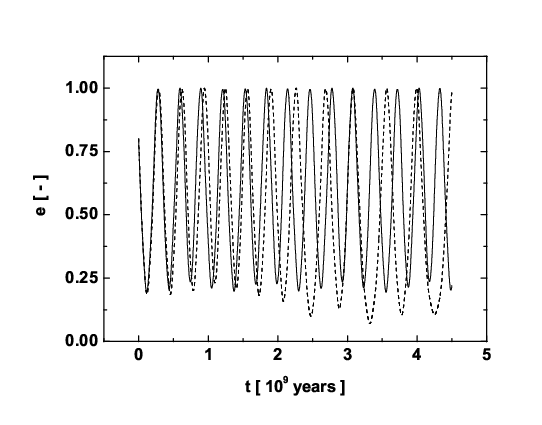
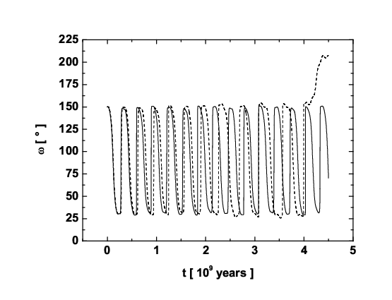
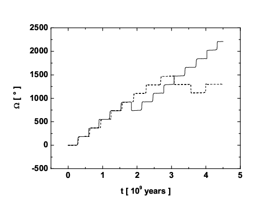
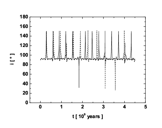
Figure 6: Two orbital evolutions of a comet with initial semi-major axis 50000 AU obtained from numerical solution of system of differential equations given by Eqs. (13)-(17) with the new terms (solid line) and without new terms (dashed line).

In Fig. 3 is compared solution of equation of motion Eq. (1) with solution of system of differential equations given by Eqs. (13)-(17). In both numerical solutions are the new term included. Evolution depicted by a solid line is obtained from solution of Eqs. (1) and evolution depicted by a dashed line is obtained from solution of Eqs. (13)-(17). Initial values of the orbital elements are ai​na_{in} == 10 000 AU, ei​ne_{in} == 0.3, ωi​n\omega_{in} == 60∘, Ωi​n\Omega_{in} == 45∘ and ii​ni_{in} == 45∘. The Sun is located at distance 8 kpc from the galactic center, Z0​(0)Z_{0}(0) == 30 pc and Z˙0​(0)\dot{Z}_{0}(0) == 7.3 km s-1, at the time tt == 0. Initial true anomaly for the evolution obtained from numerical solution of Eqs. (1) is fi​nf_{in} == 0. Orbital evolutions obtained from numerical solutions are in good accordance.

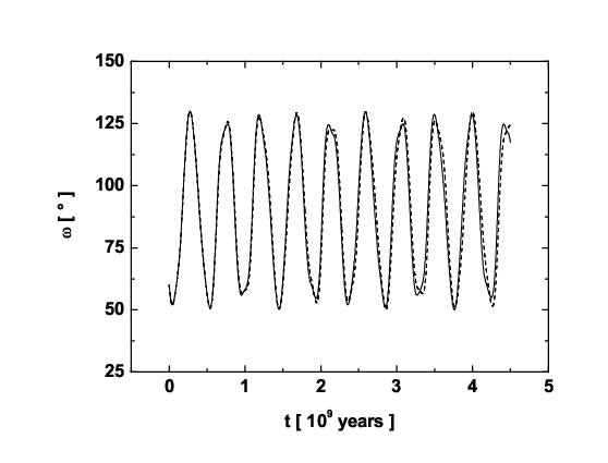
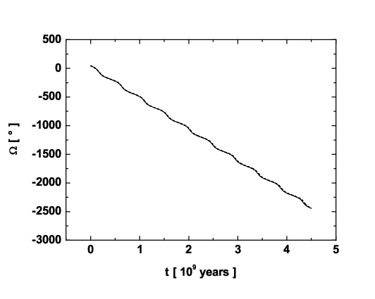
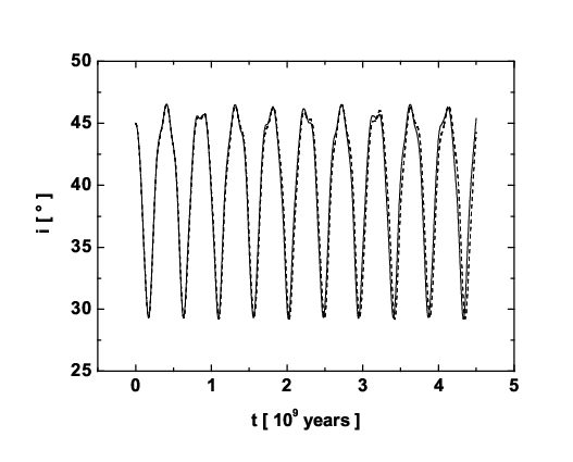
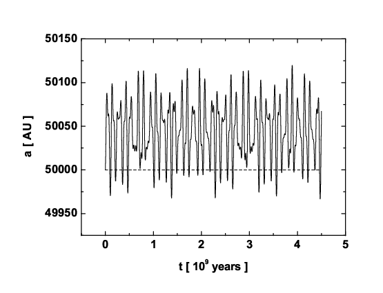
We used semi-major axis ai​na_{in} == 50000 AU for a comparison of numerical solutions of Eq. (1) and Eqs. (13)-(17) with the new terms at greater semi-major axes. Initial values of other cometary orbital elements and solar initial position and velocity are the same as for the evolutions depicted in Fig. 3. Results are depicted in Fig. 4. Difference between two evolutions is caused by the large value of the initial semi-major axis of the comet. The initial semi-major axis is so large that the orbital period of the comet (TT ≈\approx 1.1 ×\times 107 years) is comparable with the period of oscillations of the Sun around the galactic equator (2π/ωz\pi/\omega_{z} ≈\approx 7.3 ×\times 107 years). Secular orbital evolution given by Eqs. (13)-(17) cannot be used in this case.

We compared also influence of the new terms on secular evolution of orbital elements at larger semi-major axis for the initial conditions corresponding to those used in Fig. 4. The resulting evolutions are presented in Fig. 5. Evolution depicted by a solid line is for Eqs. (13)-(17) with the new terms and evolution depicted by a dashed line is for Eqs. (13)-(17) without the new terms. Evolution depicted by the solid line in Fig. 5 is identical to the evolution depicted by the dashed line in Fig. 4. Comparison of Figs. 5 and 4 shows that the influence of the new terms in Eqs. (13)-(17) on orbital evolution is less significant than motion of the Sun which was neglected in derivation of Eqs. (13)-(17).

Fig. 6 depicts numerical integration of Eqs. (13)-(17) for the case when inclusion of the new terms plays a relevant role. The new terms significantly changed the cometary orbital evolution in comparison with the orbital evolution without the new terms. Both evolutions depicted in Fig. 6 had equal initial conditions. Initial values of the comet’s orbital elements were ai​na_{in} == 50 000 AU, ei​ne_{in} == 0.8, ωi​n\omega_{in} == 150∘, Ωi​n\Omega_{in} == 0 and ii​ni_{in} == 90∘. The Sun was located at distance 8 kpc from the galactic center, Z0​(0)Z_{0}(0) == 30 pc and Z˙0​(0)\dot{Z}_{0}(0) == 7.3 km s-1, at the time tt == 0. Influence of the new terms can be even more significant for larger semi-major axis of the comet.

5 Conclusion

The paper treats the effect of the galactic tide on motion of a comet with respect to the Sun. It turns out that the important effect from the galactic tide is the action of the normal z−z-component. The x−x- and y−y- components of the acceleration comes not only from the x−x- and y−y- positional components of the comet, but also from the z−z-component of the position. This is generated by the galactic disk. The effect of the three positional components in the x−x- and y−y- acceleration components are of comparable importance.

The inclusion of the new terms into the equation of motion of the comet leads to orbital evolution which may significantly differ from the conventional result. This is true mainly for the comets with large semi-major axes. The conventional result (see, e. g. Fouchard et al. 2008) is obtained from Eqs. (13)-(17) putting Γ1\Gamma_{1} == 0, Γ2\Gamma_{2} == 0 and ϱ′\varrho^{\prime} == 0.

The solution of Eqs. (13)-(17) is in a good agreement with the solution of the equation of motion represented by Eqs. (1), if TT ≪\ll ( 1 / TzT_{z} ++ 1 / T0T_{0} )-1.

We found that a comet with the argument of perihelion ω\omega has the same orbital evolution as a comet with the argument of perihelion ω\omega ++ π\pi, if values of other orbital elements are equal. Similarly, a comet with the argument of perihelion ω\omega and the longitude of the ascending node Ω\Omega has exactly opposite time derivatives of the orbital elements as a comet with the argument of perihelion π\pi −- ω\omega and the longitude of ascending node π\pi −- Ω\Omega, if values of other orbital elements are equal.

Acknowledgement

This work was supported by the Scientific Grant Agency VEGA, Slovak Republic, grant No. 2/0016/09.

References

  • (1) Fouchard, M., Froeschlé, C., Breiter, S., Ratajczak, R., Valsecchi, G.B., Rickman, H.: Methods for the study of the dynamics of the Oort cloud comets II: Modelling the galactic tide. Lect. Notes Phys. 729, 273-296 (2008)
  • (2) Fouchard, M., Froeschlé, C., Matese, J.J., Valsecchi, G.: Comparison between different models of galactic tidal effects on cometary orbits. Celest. Mech. and Dynam. Astron. 93, 229-262 (2005)
  • (3) Klačka, J.: Electromagnetic radiation and motion of a particle. Celest. Mech. and Dynam. Astron. 89, 1-61 (2004)
  • (4) Klačka, J.: Galactic tide. arXiv:astro-ph/0912.3112 (2009a)
  • (5) Klačka, J.: Galactic tide in a noninertial frame of reference. arXiv:astro-ph/0912.3114 (2009b)
  • (6) Klačka, J., Gajdošík, M.: Orbital motion in outer Solar System. In: Pretka-Ziomek, H., Wnuk, E., Seidelmann, P.K., Richardson, D. (eds.) Dynamics of Natural and Artificial Celestial Bodies, pp. 347-349. Kluwer Academic Press, Dordrecht, arXiv:astro-ph/9910041 (2001)
  • (7) Kómar, L., Klačka, J., Pástor, P.: Galactic tide and orbital evolution of comets. arXiv:astro-ph/0912.3447 (2009)