跳到论文正文
W Papers独立论文阅读器 arXiv:0912.3312 论文正文 计算阅读时间 · 0%
引用这篇论文根据当前论文元数据生成,正式投稿前建议核对。


License: arXiv.org perpetual non-exclusive license
arXiv:0912.3312v2 [math.AC] 23 Apr 2013

Counting reducible, powerful, and relatively irreducible multivariate polynomials
over finite fields

Joachim von zur Gathen22 2 B-IT, Universität Bonn, D-53113 Bonn, Germany, {gathen,zieglerk}@bit.uni-bonn.de    Alfredo Viola33 3 Instituto de Computación, Universidad de la República, Montevideo, Uruguay, viola@fing.edu.uy    Konstantin Ziegler22 2 B-IT, Universität Bonn, D-53113 Bonn, Germany, {gathen,zieglerk}@bit.uni-bonn.de
Abstract

We present counting methods for some special classes of multivariate polynomials over a finite field, namely the reducible ones, the ss-powerful ones (divisible by the ssth power of a nonconstant polynomial), and the relatively irreducible ones (irreducible but reducible over an extension field). One approach employs generating functions, another one uses a combinatorial method. They yield exact formulas and approximations with relative errors that essentially decrease exponentially in the input size.

††footnotetext: An Extended Abstract of this paper appeared as von zur Gathen et al. (2010) and the full version is to appear in SIAM Journal of Discrete Mathematics. Dedicated to the memory of Philippe Flajolet Keywords. multivariate polynomials, finite fields, combinatorics on polynomials, counting problems, generating functions, analytic combinatorics 2010 Mathematics Subject Classification. 11T06, 12Y05, 05A15

1 Introduction

Most integers are composite and most univariate polynomials over a finite field are reducible. The classical results of the Prime Number Theorem and a theorem of Gauß present approximations saying that randomly chosen integers up to xx or polynomials of degree up to nn are prime or irreducible with probability about 1/ln⁡x1/\ln x or 1/n1/n, respectively.

Concerning special classes of univariate polynomials over a finite field, Zsigmondy (1894) counts those with a given number of distinct roots or without irreducible factors of a given degree. In the same situation, Artin (1924) counts the irreducible ones in an arithmetic progression and Hayes (1965) generalizes these results. Cohen (1969) and Car (1987) count polynomials with certain factorization patterns and Williams (1969) those with irreducible factors of given degree. Polynomials that occur as a norm in field extensions are studied by Gogia & Luthar (1981).

In two or more variables, the situation changes dramatically. Most multivariate polynomials are irreducible. Carlitz (1963) provides the first count of irreducible multivariate polynomials. In Carlitz (1965), he goes on to study the fraction of irreducibles when bounds on the degrees in each variable are prescribed; see also Cohen (1968). In this paper, we opt for bounding the total degree because it has the charm of being invariant under invertible linear transformations. Gao & Lauder (2002) consider our problem in yet another model, namely where one variable occurs with maximal degree. The natural generating function (or zeta function) for the irreducible polynomials in two or more variables does not converge anywhere outside of the origin. Wan (1992) notes that this explains the lack of a simple combinatorial formula for the number of irreducible polynomials. But he gives a pp-adic formula, and also a (somewhat complicated) combinatorial formula. For further references, see Mullen & Panario (2013, Section 3.6).

In the bivariate case, von zur Gathen (2008) proves precise approximations with an exponentially decreasing relative error. Bodin (2008) gives a recursive formula for the number of irreducible bivariate polynomials and remarks on a generalization for more than two variables; he follows up with Bodin (2010). Some further types of multivariate polynomials are examined from a counting perspective: decomposable ones (von zur Gathen (2010), Bodin et al. (2009)), singular ones (von zur Gathen (2008)), and pairs of coprime polynomials (Hou & Mullen (2009)).

This paper provides exact formulas for the numbers of reducible, ss-powerful, and relatively irreducible polynomials. The latter also yields the number of absolutely reducible polynomials. Of these, only reducible polynomials have been treated in the literature, usually with much larger error terms. The formulas yield simple, yet precise, approximations to these numbers, with rapidly decaying relative errors.

We use two different methodologies to obtain such bounds: generating functions and combinatorial counting. The usual approach, see Flajolet & Sedgewick (2009), of analytic combinatorics on series with integer coefficients leads, in our case, to power series that diverge everywhere (except at 00). We have not found a way to make this work. Instead, we use power series with symbolic coefficients, namely rational functions in a variable representing the field size. Several useful relations from standard analytic combinatorics carry over to this new scenario. In a first step, this yields in a straightforward manner exact formulas for the numbers under consideration (Theorems 3.11, 5.2, and 6.16). These formulas are, however, not very transparent. Even the leading term is not immediately visible.

In a second step, coefficient comparisons yield easy-to-use approximations to our numbers (Theorems 3.41, 5.29, and 6.48). The relative error is exponentially decreasing in the bit size of the data. As an example, Theorem 3.41 gives a “third order” approximation for the number of reducible polynomials, and thus a “fourth order” approximation for the irreducible ones. The error term is in the big-Oh form and thus contains an unspecified constant.

In a third step, a different method, namely some combinatorial counting, yields “second order” approximations with explicit constants in the error term (Theorems 4.4, 5.68, and 6.59).

Geometrically, a single polynomial corresponds to a hypersurface, that is, to a cycle in affine or projective space, of codimension 1. This correspondence preserves the respective notions of reducibility. Thus, Sections 3 and 4 can also be viewed as counting reducible hypersurfaces, in particular, planar curves, and Section 5 those with an ss-fold component. Reducible curves embedded in higher-dimensional spaces, parametrized by the appropriate Chow variety, are counted in Cesaratto et al. (2013).

2 Notation

We work in the polynomial ring F⁡[x1,…,xr]F[x_{1},\dots,x_{r}] in r≥1r\geq 1 variables over a field FF and consider polynomials with total degree equal to some nonnegative integer nn:

Pr,nall​(F)={f∈F⁡[x1,…,xr]:deg⁡f=n}.P_{r,n}^{\text{all}}(F)=\{f\in F[x_{1},\dots,x_{r}]\colon\deg f=n\}.

The polynomials of degree at most nn form an FF-vector space of dimension

br,n=(r+nr)=(r+n)r¯r!,b_{r,n}=\binom{r+n}{r}=\frac{(r+n)^{\underline{r}}}{r!},

where the falling factorial or Pochhammer symbol is

(r+x)r¯=(r+x)⋅(r−1+x)⋯(1+x),(r+x)^{\underline{r}}=(r+x)\cdot(r-1+x)\cdots(1+x), (2.1)

for any real xx and any nonnegative integer rr, see e.g. Knuth (1992). Over a finite field 𝔽q\mathbb{F}_{q} with qq elements, we have

#​Pr,nall​(𝔽q)=qbr,n−qbr,n−1=qbr,n​(1−q−br−1,n).\#P_{r,n}^{\text{all}}(\mathbb{F}_{q})=q^{b_{r,n}}-q^{b_{r,n-1}}=q^{b_{r,n}}(1-q^{-b_{r-1,n}}).

The property of a certain polynomial to be reducible, squareful or relatively irreducible is shared with all polynomials associated to the given one. For counting them, it is sufficient to take one representative. We choose an arbitrary monomial order, say, the degree-lexicographic one, so that the monic polynomials are those with leading coefficient 1, and write

Pr,n​(F)={f∈Pr,nall​(F):f​ is monic}.P_{r,n}(F)=\{f\in P_{r,n}^{\text{all}}(F)\colon f\text{ is monic}\}.

Then

#​Pr,n​(𝔽q)=#​Pr,nall​(𝔽q)q−1=qbr,n−1​1−q−br−1,n1−q−1.\#P_{r,n}(\mathbb{F}_{q})=\frac{\#P_{r,n}^{\text{all}}(\mathbb{F}_{q})}{q-1}=q^{b_{r,n}-1}\frac{1-q^{-b_{r-1,n}}}{1-q^{-1}}. (2.2)

The product of two monic polynomials is again monic.

Our exact formulas are derived using a generating series, the standard tool in analytic combinatorics as presented in Flajolet & Sedgewick (2009) by two experts who created large parts of the theory. We first recall a few general primitives from this theory that enable one to set up symbolic equations for generating functions starting from combinatorial specifications. A countable set 𝒞{\mathcal{C}} with a “size” function |⋅|:𝒞→ℤ≥0\lvert\cdot\rvert\colon{\mathcal{C}}\to\mathbb{Z}_{\geq 0} is called a combinatorial class if the preimage of any n∈ℤ≥0n\in\mathbb{Z}_{\geq 0} is finite. The number of elements of size nn is denoted by Cn{\mathrm{C}}_{n} and these numbers are encoded in the generating function C⁡(z){\mathrm{C}}(z) of the sequence Cn{\mathrm{C}}_{n}:

C⁡(z)=∑n≥0Cn​zn∈ℤ≥0​⟦z⟧.{\mathrm{C}}(z)=\sum_{n\geq 0}{\mathrm{C}}_{n}z^{n}\in\mathbb{Z}_{\geq 0}\left\llbracket z\right\rrbracket. (2.3)

We sometimes omit the argument zz. Before we tackle the task of counting polynomials, let us recall some basics about power series. An element in the ring of univariate power series over a ring is invertible if and only if its constant term is invertible. We call a power series original if its constant term vanishes, so that its graph passes through the origin. The power series

log(1−z)=−∑n≥1znn∈ℚ⟦z⟧\log(1-z)=-\sum_{n\geq 1}\frac{z^{n}}{n}\in\mathbb{Q}\left\llbracket z\right\rrbracket (2.4)

is original and substituting a power series ff in another power series gg is well-defined if ff is original.

Two combinatorial classes 𝒜{\mathcal{A}} and ℬ{\mathcal{B}} are isomorphic if there is a size-preserving bijection 𝒜→ℬ{\mathcal{A}}\to{\mathcal{B}} or equivalently if A=B{\mathrm{A}}={\mathrm{B}}. We recall three basic constructions of new combinatorial classes from given ones; see Flajolet & Sedgewick (2009, Section I. 2.).

Let 𝒜{\mathcal{A}} and ℬ{\mathcal{B}} be two combinatorial classes. We define the disjoint union

𝒜​∪˙​ℬ={{0}×𝒜}∪{{1}×ℬ}.{\mathcal{A}}\,\dot{\cup}\,{\mathcal{B}}=\{\{0\}\times{\mathcal{A}}\}\cup\{\{1\}\times{\mathcal{B}}\}. (2.5)

The size of an element (0,a)(0,a) or (1,b)(1,b) is defined as the size of aa or bb, respectively. We also define the sequence class

𝒮ℰ𝒬(𝒜)={(α1,…,αℓ):ℓ≥0,αi∈𝒜},{\mathcal{SEQ}}({\mathcal{A}})=\{(\alpha_{1},\dots,\alpha_{\ell})\colon\ell\geq 0,\alpha_{i}\in{\mathcal{A}}\}, (2.6)

where |(α1,…,αℓ)|=∑i|αi|\lvert(\alpha_{1},\dots,\alpha_{\ell})\rvert=\sum_{i}\lvert\alpha_{i}\rvert. This is a combinatorial class, if 𝒜{\mathcal{A}} contains no element of size 00. Finally, we derive the multiset class

ℳ𝒮ℰ𝒯(𝒜)=𝒮ℰ𝒬(𝒜)/∼,{\mathcal{MSET}}({\mathcal{A}})={\mathcal{SEQ}}({\mathcal{A}})/\mathbin{\sim}, (2.7)

where (α1,…,αℓ)∼(β1,…,βℓ)(\alpha_{1},\dots,\alpha_{\ell})\sim(\beta_{1},\dots,\beta_{\ell}) if there is a permutation σ\sigma of {1,…,ℓ}\{1,\dots,\ell\} such that αi=βσ⁡(i)\alpha_{i}=\beta_{\sigma(i)} for all ii. This class contains all finite sequences of elements from 𝒜{\mathcal{A}} where repetition is allowed, but ordering ignored. The generating functions for these constructions are classic applications of combinatorics.

2.8see Flajolet & Sedgewick (2009, Theorems I.1 and I.5).

Let 𝒜{\mathcal{A}}, ℬ{\mathcal{B}}, and 𝒞{\mathcal{C}} be combinatorial classes.

  1. (i)

    If 𝒜=ℬ​∪˙​𝒞{\mathcal{A}}={\mathcal{B}}\,\dot{\cup}\,{\mathcal{C}}, then A=B+C{\mathrm{A}}={\mathrm{B}}+{\mathrm{C}}.

  2. (ii)

    If 𝒜=ℳ​𝒮​ℰ​𝒯​(ℬ){\mathcal{A}}={\mathcal{MSET}}({\mathcal{B}}) and B0=0{\mathrm{B}}_{0}=0, then

    B=∑k≥1μ⁡(k)k​log⁡(A⁡(zk)),{\mathrm{B}}=\sum_{k\geq 1}\frac{\mu(k)}{k}\log({\mathrm{A}}(z^{k})), (2.9)

    where μ\mu is the number-theoretic Möbius-function, defined as

    μ⁡(k)={1if k=1,(−1)ℓif k is the product of ℓ distinct primes,0otherwise.\mu(k)=\begin{cases}1&if $k=1$,\\ (-1)^{\ell}&if $k$ is the product of $\ell$ distinct primes,\\ 0&otherwise.\end{cases} (2.10)

3 Generating functions for reducible polynomials

To study reducible polynomials, we consider the following subsets of Pr,n​(F)P_{r,n}(F):

Ir,n​(F)\displaystyle I_{r,n}(F) ={f∈Pr,n​(F):f​ irreducible},\displaystyle=\{f\in P_{r,n}(F)\colon f\textrm{ irreducible}\},
Rr,n​(F)\displaystyle R_{r,n}(F) =Pr,n​(F)∖Ir,n​(F).\displaystyle=P_{r,n}(F)\setminus I_{r,n}(F).

In the usual notions, the polynomial 11 is neither reducible nor irreducible. In our context, it is natural to have Rr,0​(F)={1}R_{r,0}(F)=\{1\} and Ir,0​(F)=∅I_{r,0}(F)=\varnothing.

The sets of polynomials

𝒫\displaystyle{\mathcal{P}} =⋃n≥0Pr,n​(𝔽q),\displaystyle=\bigcup_{n\geq 0}P_{r,n}(\mathbb{F}_{q}), (3.1)
ℐ\displaystyle{\mathcal{I}} =⋃n≥0Ir,n​(𝔽q),\displaystyle=\bigcup_{n\geq 0}I_{r,n}(\mathbb{F}_{q}), (3.2)
ℛ\displaystyle{\mathcal{R}} =𝒫∖ℐ,\displaystyle={\mathcal{P}}\setminus{\mathcal{I}}, (3.3)

are combinatorial classes with the total degree as size functions and we denote the corresponding generating functions by P,I,R∈ℤ≥0​⟦z⟧{\mathrm{P}},{\mathrm{I}},{\mathrm{R}}\in\mathbb{Z}_{\geq 0}\left\llbracket z\right\rrbracket, respectively. Their coefficients are

Pn\displaystyle{\mathrm{P}}_{n} =Pr,n​(𝔽q)=#​Pr,n​(𝔽q)=qbr,n−1​1−q−br−1,n1−q−1,\displaystyle={\mathrm{P}}_{r,n}(\mathbb{F}_{q})=\#P_{r,n}(\mathbb{F}_{q})=q^{b_{r,n}-1}\frac{1-q^{-b_{r-1,n}}}{1-q^{-1}}, (3.4)
Rn\displaystyle{\mathrm{R}}_{n} =Rr,n​(𝔽q)=#​Rr,n​(𝔽q),\displaystyle={\mathrm{R}}_{r,n}(\mathbb{F}_{q})=\#R_{r,n}(\mathbb{F}_{q}), (3.5)
In\displaystyle{\mathrm{I}}_{n} =Ir,n​(𝔽q)=#​Ir,n​(𝔽q),\displaystyle={\mathrm{I}}_{r,n}(\mathbb{F}_{q})=\#I_{r,n}(\mathbb{F}_{q}), (3.6)

respectively, dropping 𝔽q\mathbb{F}_{q} and rr from the notation. By definition, 𝒫{\mathcal{P}} is isomorphic to the disjoint union of ℛ{\mathcal{R}} and ℐ{\mathcal{I}}, and therefore

R=P−I{\mathrm{R}}={\mathrm{P}}-{\mathrm{I}} (3.8)

by 2.8 (i). By unique factorization, every element in 𝒫{\mathcal{P}} corresponds to an unordered finite sequence of irreducible polynomials, where repetition is allowed. Hence 𝒫{\mathcal{P}} is isomorphic to ℳ​𝒮​ℰ​𝒯​(ℐ){\mathcal{MSET}}({\mathcal{I}}) and by 2.8 (ii),

I=∑k≥1μ⁡(k)k​log⁡P⁡(zk).{\mathrm{I}}=\sum_{k\geq 1}\frac{\mu(k)}{k}\log{\mathrm{P}}(z^{k}). (3.9)

A Maple implementation of the resulting algorithm to compute the number of reducible polynomials is described in Figure 1. It is easy to program and execute and was used to calculate the number of bivariate reducible polynomials in von zur Gathen (2008, Table 2.1). We extend these exact results in Table 1.

allpolysGF:=proc(z,N,r) local i: option remember: sum(’simplify((qˆbinomial(r+i,r)-qˆbinomial(r+i-1,r))/ (q-1))*zˆi’,i = 0..N):end:irreduciblesGF:=proc(z,N,r) local k: option remember: convert(taylor((sum(’mobius(k)/k*log(allpolysGF(zˆk,N,r))’, k=1..N)), z, N+1), polynom):end:reduciblesGF:=proc(z,N,r) option remember: allpolysGF(z,N,r)-irreduciblesGF(z,N,r):end:reducibles:=proc(n,r)coeff(sort(expand(reduciblesGF(z,n,r))),zˆn):end:

Figure 1: Maple program to compute the number of monic reducible polynomials in rr variables of degree nn.

Table 1: Exact values of #​Rr,n​(𝔽q)\#R_{r,n}(\mathbb{F}_{q}) for small values of rr and nn. For n<4n<4, these are the numbers given in Theorem 3.41.

This approach quickly leads to explicit formulas. For a positive integer nn, a composition of nn is a sequence j=(j1,j2,…,j|j|)j=(j_{1},j_{2},\dots,j_{\lvert j\rvert}) of positive integers j1,j2,…,j|j|j_{1},j_{2},\dots,j_{\lvert j\rvert} with j1+j2+⋯+j|j|=nj_{1}+j_{2}+\dots+j_{\lvert j\rvert}=n, where |j|\lvert j\rvert denotes the length of the sequence. We define the set

Mn={compositions of n}.M_{n}=\{\text{compositions of $n$}\}. (3.10)

This standard combinatorial notion is not to be confused with the composition of polynomials, for which also counting results are available.

3.11.

For r≥1r\geq 1, q≥2q\geq 2, and Pn{\mathrm{P}}_{n} as in (3.4), we have

I0=0,In=−∑k|nμ⁡(k)k∑j∈Mn/k(−1)|j||j|Pj1Pj2⋯Pj|j|,\begin{split}{\mathrm{I}}_{0}&=0,\\ {\mathrm{I}}_{n}&=-\sum_{k\,\mid\,n}\frac{\mu(k)}{k}\sum_{j\in M_{n/k}}\frac{(-1)^{\lvert j\rvert}}{\lvert j\rvert}{\mathrm{P}}_{j_{1}}{\mathrm{P}}_{j_{2}}\cdots{\mathrm{P}}_{j_{\lvert j\rvert}},\end{split} (3.12)

for n≥1n\geq 1, and therefore

R0\displaystyle{\mathrm{R}}_{0} =1,\displaystyle=1, (3.13)
Rn\displaystyle{\mathrm{R}}_{n} =Pn+∑k|nμ⁡(k)k∑j∈Mn/k(−1)|j||j|Pj1Pj2⋯Pj|j|,\displaystyle={\mathrm{P}}_{n}+\sum_{k\,\mid\,n}\frac{\mu(k)}{k}\sum_{j\in M_{n/k}}\frac{(-1)^{\lvert j\rvert}}{\lvert j\rvert}{\mathrm{P}}_{j_{1}}{\mathrm{P}}_{j_{2}}\cdots{\mathrm{P}}_{j_{\lvert j\rvert}}, (3.14)

for n≥1n\geq 1.

Proof.

We consider the original power series F=1−𝖯=−∑i≥1Pizi{\mathrm{F}}=1-{\mathsf{P}}=-\sum_{i\geq 1}{\mathrm{P}}_{i}z^{i}. The Taylor expansion (2.4) of log⁡(1−F⁡(zk))\log(1-{\mathrm{F}}(z^{k})) in (3.9) yields

I\displaystyle{\mathrm{I}} =−∑k≥1μ⁡(k)k∑i≥1F​(zk)ii=−∑k≥1μ⁡(k)k∑i≥1(−1)ii(∑j≥1Pjzj​k)i\displaystyle=-\sum_{k\geq 1}\frac{\mu(k)}{k}\sum_{i\geq 1}\frac{{\mathrm{F}}(z^{k})^{i}}{i}=-\sum_{k\geq 1}\frac{\mu(k)}{k}\sum_{i\geq 1}\frac{(-1)^{i}}{i}\Bigl(\sum_{j\geq 1}{\mathrm{P}}_{j}z^{jk}\Bigr)^{i} (3.15)
=−∑k≥1μ⁡(k)k∑i≥1(−1)ii(P1zk+P2z2​k+P3z3​k+…)i,\displaystyle=-\sum_{k\geq 1}\frac{\mu(k)}{k}\sum_{i\geq 1}\frac{(-1)^{i}}{i}({\mathrm{P}}_{1}z^{k}+{\mathrm{P}}_{2}z^{2k}+{\mathrm{P}}_{3}z^{3k}+\dots)^{i}, (3.16)
I0\displaystyle{\mathrm{I}}_{0} =0,\displaystyle=0, (3.17)
In\displaystyle{\mathrm{I}}_{n} =−∑k|nμ⁡(k)k∑i≥1(−1)ii∑j∈Mn/k|j|=iPj1Pj2⋯Pji,\displaystyle=-\sum_{k\,\mid\,n}\frac{\mu(k)}{k}\sum_{i\geq 1}\frac{(-1)^{i}}{i}\sum_{\begin{subarray}{c}j\in M_{n/k}\\ \lvert j\rvert=i\end{subarray}}{\mathrm{P}}_{j_{1}}{\mathrm{P}}_{j_{2}}\cdots{\mathrm{P}}_{j_{i}}, (3.18)

for n≥1n\geq 1, which proves the claimed formulas for I{\mathrm{I}}. The results for R{\mathrm{R}} follow by (3.8). ∎

We check that the formula yields the well-known one, see Lidl & Niederreiter (1997, Theorem 3.25), in the univariate case, where r=1r=1. We then have Pj=qj{\mathrm{P}}_{j}=q^{j} and so Pj1Pj2⋯Pji=qn/k{\mathrm{P}}_{j_{1}}{\mathrm{P}}_{j_{2}}\cdots{\mathrm{P}}_{j_{i}}=q^{n/k} for any composition j1+j2+⋯+ji=n/kj_{1}+j_{2}+\dots+j_{i}=n/k. Moreover, the number of compositions of mm with ii components is (m−1i−1)\binom{m-1}{i-1}, see Flajolet & Sedgewick (2009, Section I.3.1). As a consequence we have for kk dividing nn

∑j∈Mn/k|j|=i(−1)iiPj1Pj2⋯Pji\displaystyle\sum_{\begin{subarray}{c}j\in M_{n/k}\\ \lvert j\rvert=i\end{subarray}}\frac{(-1)^{i}}{i}{\mathrm{P}}_{j_{1}}{\mathrm{P}}_{j_{2}}\cdots{\mathrm{P}}_{j_{i}} =qn/k​∑i≥1(−1)ii​(n/k−1i−1)\displaystyle=q^{n/k}\sum_{i\geq 1}\frac{(-1)^{i}}{i}\binom{n/k-1}{i-1} (3.19)
=k​qn/kn​∑i≥1(−1)i​(n/ki)=−k​qn/kn,\displaystyle=\frac{kq^{n/k}}{n}\sum_{i\geq 1}(-1)^{i}\binom{n/k}{i}=-\frac{kq^{n/k}}{n}, (3.20)
In\displaystyle{\mathrm{I}}_{n} =1n​∑k|nμ⁡(k)​qn/k.\displaystyle=\frac{1}{n}\sum_{k\,\mid\,n}\mu(k)q^{n/k}. (3.21)

Cohen (1968) notes that, compared to the univariate case, “the situation is different and much more difficult. In this case, no explicit formula […] is available.”

For r≥2r\geq 2, the power series P{\mathrm{P}}, I{\mathrm{I}}, and R{\mathrm{R}} do not converge anywhere except at 0, and the standard asymptotic arguments of analytic combinatorics are inapplicable. We now deviate from this approach and move from power series in ℚ​⟦z⟧\mathbb{Q}\left\llbracket z\right\rrbracket to power series in ℚ⁡(𝐪)​⟦z⟧\mathbb{Q}(\mathbf{q})\left\llbracket z\right\rrbracket, where 𝐪\mathbf{q} is a symbolic variable representing the field size. For r≥2r\geq 2 and n≥0n\geq 0 we let

𝖯n​(𝐪)=𝖯r,n​(𝐪)=𝐪br,n−1​1−𝐪−br−1,n1−𝐪−1∈ℤ⁡[𝐪],{\mathsf{P}}_{n}(\mathbf{q})={\mathsf{P}}_{r,n}(\mathbf{q})=\mathbf{q}^{b_{r,n}-1}\frac{1-\mathbf{q}^{-b_{r-1,n}}}{1-\mathbf{q}^{-1}}\in\mathbb{Z}[\mathbf{q}], (3.22)

where we usually omit rr from the notation. As examples, we have

𝖯0​(𝐪)=1,𝖯1​(𝐪)=𝐪r​1−𝐪−r1−𝐪−1, and ​𝖯2​(𝐪)=𝐪r⁡(r+3)/2​1−𝐪−r(r+1)/21−𝐪−1.{\mathsf{P}}_{0}(\mathbf{q})=1,{\mathsf{P}}_{1}(\mathbf{q})=\mathbf{q}^{r}\frac{1-\mathbf{q}^{-r}}{1-\mathbf{q}^{-1}},\text{ and }{\mathsf{P}}_{2}(\mathbf{q})=\mathbf{q}^{r(r+3)/2}\frac{1-\mathbf{q}^{-r(r+1)/2}}{1-\mathbf{q}^{-1}}. (3.23)

We define the power series 𝖯,𝖨,𝖱∈ℚ⁡(𝐪)​⟦z⟧{\mathsf{P}},{\mathsf{I}},{\mathsf{R}}\in\mathbb{Q}(\mathbf{q})\left\llbracket z\right\rrbracket by

𝖯⁡(𝐪,z)\displaystyle{\mathsf{P}}(\mathbf{q},z) =∑n≥0𝖯n​(𝐪)​zn,\displaystyle=\sum_{n\geq 0}{\mathsf{P}}_{n}(\mathbf{q})z^{n}, (3.24)
𝖨⁡(𝐪,z)\displaystyle{\mathsf{I}}(\mathbf{q},z) =∑k≥1μ⁡(k)k​log⁡𝖯⁡(𝐪,zk),\displaystyle=\sum_{k\geq 1}\frac{\mu(k)}{k}\log{\mathsf{P}}(\mathbf{q},z^{k}), (3.25)
𝖱⁡(𝐪,z)\displaystyle{\mathsf{R}}(\mathbf{q},z) =𝖯⁡(𝐪,z)−𝖨⁡(𝐪,z).\displaystyle={\mathsf{P}}(\mathbf{q},z)-{\mathsf{I}}(\mathbf{q},z). (3.26)

Now 1−𝖯⁡(𝐪,zk)1-{\mathsf{P}}(\mathbf{q},z^{k}) is an original power series, and log⁡𝖯⁡(𝐪,zk)\log{\mathsf{P}}(\mathbf{q},z^{k}) and 𝖨{\mathsf{I}} are well-defined, with 𝖨⁡(𝐪,0)=0{\mathsf{I}}(\mathbf{q},0)=0. For q∈ℚq\in\mathbb{Q}, the rational functions in ℚ⁡(𝐪)\mathbb{Q}(\mathbf{q}) without pole at 𝐪←q\mathbf{q}\leftarrow q form a ring, the localization ℚ​[𝐪](𝐪−q)\mathbb{Q}[\mathbf{q}]_{(\mathbf{q}-q)}. If we restrict the power series coefficients to this ring, the evaluation map which substitutes an integer qq for 𝐪\mathbf{q} is a ring homomorphism. Since 𝖯n{\mathsf{P}}_{n} is actually a polynomial in 𝐪\mathbf{q}, this poses no restriction in our case, and evaluating 𝐪←q\mathbf{q}\leftarrow q maps 𝖯⁡(𝐪,z){\mathsf{P}}(\mathbf{q},z) to P⁡(z){\mathrm{P}}(z) coefficientwise. In other words, the coefficient of znz^{n} equals

[zn]​𝖯​(q,z)=Pn[z^{n}]{\mathsf{P}}(q,z)={\mathrm{P}}_{n} (3.27)

by (2.2). Furthermore, 𝖨{\mathsf{I}} and 𝖱{\mathsf{R}} relate to 𝖯{\mathsf{P}} in the same way as I{\mathrm{I}} and R{\mathrm{R}} do to P{\mathrm{P}}, so that

[zn]​𝖨​(q,z)=In,\displaystyle[z^{n}]{\mathsf{I}}(q,z)={\mathrm{I}}_{n}, (3.28)
[zn]​𝖱​(q,z)=Rn.\displaystyle[z^{n}]{\mathsf{R}}(q,z)={\mathrm{R}}_{n}. (3.29)

The formula of Theorem 3.11 is exact but somewhat cumbersome. A main goal in this work is to find simple yet precise approximations, with rapidly decaying error terms. We fix some notation. For nonzero f∈ℚ⁡(𝐪)f\in\mathbb{Q}(\mathbf{q}), deg𝐪⁡f\deg_{\mathbf{q}}f is the degree of ff, that is, the numerator degree minus the denominator degree. Thus deg𝐪⁡𝖯n=br,n−1\deg_{\mathbf{q}}{\mathsf{P}}_{n}=b_{r,n}-1 and deg𝐪⁡(f+g)≤max⁡{deg𝐪⁡f,deg𝐪⁡g}\deg_{\mathbf{q}}(f+g)\leq\max\{\deg_{\mathbf{q}}f,\deg_{\mathbf{q}}g\}. The appearance of O⁡(𝐪−m)O(\mathbf{q}^{-m}) with a positive integer mm in an equation means the existence of some ff with degree at most −m-m that makes the equation valid. The charm of our approach is that we obtain results for any “fixed” rr and nn. If a term O⁡(𝐪−m)O(\mathbf{q}^{-m}) appears, then we may conclude a numerical asymptotic result for growing prime powers qq.

We start with a degree comparison for certain products of the 𝖯i​(𝐪){\mathsf{P}}_{i}(\mathbf{q}) and sometimes omit the argument 𝐪\mathbf{q}.

3.30.

Let r≥2r\geq 2 and n≥0n\geq 0.

  1. (i)

    For i,j≥0i,j\geq 0, we have deg𝐪⁡(𝖯i⋅𝖯j)≤deg𝐪⁡𝖯i+j\deg_{\mathbf{q}}({\mathsf{P}}_{i}\cdot{\mathsf{P}}_{j})\leq\deg_{\mathbf{q}}{\mathsf{P}}_{i+j}, with equality if and only if i​j=0ij=0.

  2. (ii)

    For 1≤k≤n/21\leq k\leq n/2, the sequence of integers deg𝐪⁡(𝖯k⋅𝖯n−k)\deg_{\mathbf{q}}({\mathsf{P}}_{k}\cdot{\mathsf{P}}_{n-k}) is strictly decreasing in kk.

  3. (iii)

    For 3≤k≤n/23\leq k\leq n/2, we have deg𝐪⁡𝖯12​𝖯n−2≥deg𝐪⁡𝖯k​𝖯n−k\deg_{\mathbf{q}}{\mathsf{P}}_{1}^{2}{\mathsf{P}}_{n-2}\geq\deg_{\mathbf{q}}{\mathsf{P}}_{k}{\mathsf{P}}_{n-k}, with equality only for (r,n,k)=(2,6,3)(r,n,k)=(2,6,3).

Proof.
  1. (i)

    The claimed inequality is equivalent to

    (r+ir)+(r+jr)−1≤(r+i+jr),\binom{r+i}{r}+\binom{r+j}{r}-1\leq\binom{r+i+j}{r}, (3.31)

    which follows by considering the choices of rr-element subsets from a set with r+i+jr+i+j elements. Since r≥2r\geq 2, this inequality is strict if and only if both ii and jj are nonzero.

  2. (ii)

    Using (3.22), we define a function uu as

    u⁡(k)=deg𝐪⁡(𝖯k⋅𝖯n−k)=(r+kr)+(r+n−kr)−2.u(k)=\deg_{\mathbf{q}}({\mathsf{P}}_{k}\cdot{\mathsf{P}}_{n-k})=\binom{r+k}{r}+\binom{r+n-k}{r}-2. (3.32)

    We extend the domain of u⁡(k)u(k) to real numbers kk between 11 and n/2n/2 by means of falling factorials as in (2.1)

    u⁡(k)=(r+k)r¯r!+(r+n−k)r¯r!−2.u(k)=\frac{(r+k)^{\underline{r}}}{r!}+\frac{(r+n-k)^{\underline{r}}}{r!}-2.

    It is sufficient to show that the affine transformation u¯\bar{u} with

    u¯​(k)=r!⋅(u⁡(k)+2)=(r+k)r¯+(r+n−k)r¯\bar{u}(k)=r!\cdot(u(k)+2)=(r+k)^{\underline{r}}+(r+n-k)^{\underline{r}}

    is strictly decreasing. The first derivative with respect to kk is

    u¯′​(k)=∑1≤i≤r((r+k)r¯i+k−(r+n−k)r¯i+n−k).{\bar{u}}^{\prime}(k)=\sum_{1\leq i\leq r}\Bigl(\frac{(r+k)^{\underline{r}}}{i+k}-\frac{(r+n-k)^{\underline{r}}}{i+n-k}\Bigr). (3.33)

    Since 0<i+k<i+n−k0<i+k<i+n-k for 1<k<n/21<k<n/2, each difference is negative, and so is u¯′​(k){\bar{u}}^{\prime}(k).

  3. (iii)

    Since r≥2r\geq 2 we have

    (r−2)​(r−1)​(r+5)\displaystyle(r-2)(r-1)(r+5) ≥0,\displaystyle\geq 0, (3.34)
    br−1,4\displaystyle b_{r-1,4} ≥br,3−2​r−1,\displaystyle\geq b_{r,3}-2r-1, (3.35)
    2​r+br,4−1\displaystyle 2r+b_{r,4}-1 ≥2​br,3−2,\displaystyle\geq 2b_{r,3}-2, (3.36)
    deg𝐪⁡𝖯12​𝖯4\displaystyle\deg_{\mathbf{q}}{\mathsf{P}}_{1}^{2}{\mathsf{P}}_{4} ≥deg𝐪⁡𝖯3​𝖯3,\displaystyle\geq\deg_{\mathbf{q}}{\mathsf{P}}_{3}{\mathsf{P}}_{3}, (3.37)

    and equality if and only if r=2r=2. This proves the claimed inequality for n=6n=6.

    For n>6n>6 we have br−1,n−2>br−1,4b_{r-1,n-2}>b_{r-1,4} and with (3.35) follows

    br−1,n−2\displaystyle b_{r-1,n-2} >br,3−2​r−1,\displaystyle>b_{r,3}-2r-1, (3.38)
    2​r+br,n−2−1\displaystyle 2r+b_{r,n-2}-1 >br,3+br,n−3−2,\displaystyle>b_{r,3}+b_{r,n-3}-2, (3.39)
    deg𝐪⁡𝖯12​𝖯n−2\displaystyle\deg_{\mathbf{q}}{\mathsf{P}}_{1}^{2}{\mathsf{P}}_{n-2} >deg𝐪⁡𝖯3​𝖯n−3,\displaystyle>\deg_{\mathbf{q}}{\mathsf{P}}_{3}{\mathsf{P}}_{n-3}, (3.40)

    which proves (iii) for k=3k=3 and by the monotonicity proven in (ii) also for all larger kk. ∎

3.41.

Let r≥2r\geq 2 and

ρr,n​(𝐪)=𝐪(r+n−1r)+r−1​1−𝐪−r(1−𝐪−1)2∈ℚ⁡(𝐪).\rho_{r,n}(\mathbf{q})=\mathbf{q}^{\binom{r+n-1}{r}+r-1}\frac{1-\mathbf{q}^{-r}}{(1-\mathbf{q}^{-1})^{2}}\in\mathbb{Q}(\mathbf{q}). (3.42)

Then

𝖱0\displaystyle{\mathsf{R}_{0}} =1,\displaystyle=1, (3.43)
𝖱1\displaystyle{\mathsf{R}_{1}} =0,\displaystyle=0, (3.44)
𝖱2\displaystyle{\mathsf{R}_{2}} =ρr,2​(𝐪)2⋅(1−𝐪−r−1),\displaystyle=\frac{\rho_{r,2}(\mathbf{q})}{2}\cdot(1-\mathbf{q}^{-r-1}), (3.45)
𝖱3\displaystyle{\mathsf{R}_{3}} =ρr,3(𝐪)(1−𝐪−r(r+1)/2+𝐪−r(r−1)/21−2​𝐪−r+2​𝐪−2​r−1−𝐪−2​r−23​(1−𝐪−1)),\displaystyle=\rho_{r,3}(\mathbf{q})\Bigl(1-\mathbf{q}^{-r(r+1)/2}+\mathbf{q}^{-r(r-1)/2}\frac{1-2\mathbf{q}^{-r}+2\mathbf{q}^{-2r-1}-\mathbf{q}^{-2r-2}}{3(1-\mathbf{q}^{-1})}\Bigr), (3.46)
𝖱4\displaystyle{\mathsf{R}_{4}} =ρr,4​(𝐪)⋅(1+𝐪−(r+13)⋅1+O(𝐪−r(r−1)/2)2​(1−𝐪−r)),\displaystyle=\rho_{r,4}(\mathbf{q})\cdot\Bigl(1+\mathbf{q}^{-\binom{r+1}{3}}\cdot\frac{1+O(\mathbf{q}^{-r(r-1)/2})}{2(1-\mathbf{q}^{-r})}\Bigr), (3.47)
and for n≥5n\geq 5
𝖱n\displaystyle{\mathsf{R}_{n}} =ρr,n​(𝐪)⋅(1+𝐪−(r+n−2r−1)+r⁡(r+1)/2⋅1+O(𝐪−r(r−1)/2)1−𝐪−r).\displaystyle=\rho_{r,n}(\mathbf{q})\cdot\Bigl(1+\mathbf{q}^{-\binom{r+n-2}{r-1}+r(r+1)/2}\cdot\frac{1+O(\mathbf{q}^{-r(r-1)/2})}{1-\mathbf{q}^{-r}}\Bigr). (3.48)
Proof.

We start the symbolic analog of our approach in the proof of Theorem 3.11 with the original power series 𝖥=1−𝖯=−∑i≥1𝖯izi{\mathsf{F}}=1-{\mathsf{P}}=-\sum_{i\geq 1}{\mathsf{P}}_{i}z^{i}. The Taylor expansion of log⁡(1−𝖥⁡(zk))\log(1-{\mathsf{F}}(z^{k})) in (3.25) yields

𝖱=𝖯−𝖨=1+∑i≥2𝖥ii+∑k≥2μ⁡(k)k​∑i≥1𝖥​(zk)ii.{\mathsf{R}}={\mathsf{P}}-{\mathsf{I}}=1+\sum_{i\geq 2}\frac{{\mathsf{F}}^{i}}{i}+\sum_{k\geq 2}\frac{\mu(k)}{k}\sum_{i\geq 1}\frac{{\mathsf{F}}(z^{k})^{i}}{i}. (3.49)

Since 𝖱n=[zn]​𝖱{\mathsf{R}}_{n}=[z^{n}]{\mathsf{R}}, we find 𝖱0=1{\mathsf{R}}_{0}=1, 𝖱1=0{\mathsf{R}}_{1}=0, 𝖱2=(𝖯12+𝖯1)/2{\mathsf{R}}_{2}=({\mathsf{P}}_{1}^{2}+{\mathsf{P}}_{1})/2, and 𝖱3=𝖯2​𝖯1−(𝖯13−𝖯1)/3{\mathsf{R}}_{3}={\mathsf{P}}_{2}{\mathsf{P}}_{1}-({\mathsf{P}}_{1}^{3}-{\mathsf{P}}_{1})/3. Together with (3.23), these imply the claims for n<4n<4.

ii summands summands with
largest degree in ​𝐪\text{largest degree in }\mathbf{q}
[zn]​𝖥i[z^{n}]{\mathsf{F}}^{i} 22 𝖯j​𝖯n−j,{\mathsf{P}}_{j}{\mathsf{P}}_{n-j}, 𝖯1​𝖯n−1,𝖯2​𝖯n−2,{\mathsf{P}}_{1}{\mathsf{P}}_{n-1},{\mathsf{P}}_{2}{\mathsf{P}}_{n-2},
1≤j≤n/2\hskip 8.50012pt1\leq j\leq n/2 𝖯3​𝖯n−3​ (for n≥6)\hskip 8.50012pt{\mathsf{P}}_{3}{\mathsf{P}}_{n-3}\text{ (for $n\geq 6$)}
≥3\geq 3 𝖯j1𝖯j2⋯𝖯ji,{\mathsf{P}}_{j_{1}}{\mathsf{P}}_{j_{2}}\cdots{\mathsf{P}}_{j_{i}}, 𝖯12​𝖯n−2{\mathsf{P}}_{1}^{2}{\mathsf{P}}_{n-2}
1≤j1≤j2≤⋯≤ji≤n,\hskip 8.50012pt1\leq j_{1}\leq j_{2}\leq\dots\leq j_{i}\leq n,
j1+j2+⋯+ji=n,\hskip 8.50012ptj_{1}+j_{2}+\dots+j_{i}=n,
[zn]​𝖥​(zk)i{[z^{n}]}{\mathsf{F}}(z^{k})^{i} 11 𝖯n/k{\mathsf{P}}_{n/k} 𝖯n/k{\mathsf{P}}_{n/k}
≥2\geq 2 𝖯j1𝖯j2⋯𝖯ji,{\mathsf{P}}_{j_{1}}{\mathsf{P}}_{j_{2}}\cdots{\mathsf{P}}_{j_{i}}, 𝖯1​𝖯n/k−1{\mathsf{P}}_{1}{\mathsf{P}}_{n/k-1}
1≤j1≤j2≤⋯≤ji≤n/k,\hskip 8.50012pt1\leq j_{1}\leq j_{2}\leq\dots\leq j_{i}\leq n/k,
j1+j2​⋯+ji=n/k,\hskip 8.50012ptj_{1}+j_{2}\dots+j_{i}=n/k,
Table 2: Summands of 𝖱{\mathsf{R}} and bounds on their degrees in 𝐪\mathbf{q}.

When n≥4n\geq 4, the contributions to [zn]​𝖱[z^{n}]{\mathsf{R}} from both sums in (3.49) are displayed in Table 2, distinguishing the smallest possible value for ii from the remaining larger ones. The third column lists all summands. We first show that the last column displays the terms of largest degree in their row, and then compare the summands in the last column. The terms of [zn]​𝖥i[z^{n}]{\mathsf{F}}^{i} are products of ii factors

𝖯j1𝖯j2⋯𝖯ji,1≤j1≤j2≤⋯≤ji≤n,{\mathsf{P}}_{j_{1}}{\mathsf{P}}_{j_{2}}\cdots{\mathsf{P}}_{j_{i}},\quad 1\leq j_{1}\leq j_{2}\leq\dots\leq j_{i}\leq n,

with j1+j2+⋯+ji=nj_{1}+j_{2}+\dots+j_{i}=n. For i=2i=2, we find

deg𝐪⁡𝖯1​𝖯n−1>deg𝐪⁡𝖯2​𝖯n−2>deg𝐪⁡𝖯j​𝖯n−j\deg_{\mathbf{q}}{\mathsf{P}}_{1}{\mathsf{P}}_{n-1}>\deg_{\mathbf{q}}{\mathsf{P}}_{2}{\mathsf{P}}_{n-2}>\deg_{\mathbf{q}}{\mathsf{P}}_{j}{\mathsf{P}}_{n-j} (3.50)

for all jj with 3≤j≤n/23\leq j\leq n/2 by 3.30 (ii). For i≥3i\geq 3,

deg𝐪𝖯12𝖯n−2≥deg𝐪𝖯j1𝖯j2⋯𝖯ji\deg_{\mathbf{q}}{\mathsf{P}}_{1}^{2}{\mathsf{P}}_{n-2}\geq\deg_{\mathbf{q}}{\mathsf{P}}_{j_{1}}{\mathsf{P}}_{j_{2}}\cdots{\mathsf{P}}_{j_{i}} (3.51)

for all admissible values of j1,…,jij_{1},\dots,j_{i} by repeated application of 3.30 (i) and a single instance of (ii). Let kk divide nn. Then [zn]​𝖥​(zk)=−𝖯n/k[z^{n}]{\mathsf{F}}(z^{k})=-{\mathsf{P}}_{n/k} and [zn]​∑i≥2𝖥​(zk)i[z^{n}]\sum_{i\geq 2}{\mathsf{F}}(z^{k})^{i} has degree deg𝐪⁡𝖯1​𝖯n/k−1\deg_{\mathbf{q}}{\mathsf{P}}_{1}{\mathsf{P}}_{n/k-1} as shown above for k=1k=1.

We continue the comparison started in (3.50) by noting that deg𝐪⁡𝖯2​𝖯n−2>deg𝐪⁡𝖯12​𝖯n−2\deg_{\mathbf{q}}{\mathsf{P}}_{2}{\mathsf{P}}_{n-2}>\deg_{\mathbf{q}}{\mathsf{P}}_{1}^{2}{\mathsf{P}}_{n-2} by 3.30 (i), and also deg𝐪⁡𝖯12​𝖯n−2≥deg𝐪⁡𝖯j​𝖯n−j\deg_{\mathbf{q}}{\mathsf{P}}_{1}^{2}{\mathsf{P}}_{n-2}\geq\deg_{\mathbf{q}}{\mathsf{P}}_{j}{\mathsf{P}}_{n-j} for all 3≤j≤n/23\leq j\leq n/2 with equality only for (r,n,j)=(2,6,3)(r,n,j)=(2,6,3) by 3.30 (iii). Furthermore, since deg𝐪⁡𝖯1≥1\deg_{\mathbf{q}}{\mathsf{P}}_{1}\geq 1, we have for k≥2k\geq 2

deg𝐪⁡𝖯12​𝖯n−2>deg𝐪⁡𝖯n−2≥deg𝐪⁡𝖯n/k>deg𝐪⁡𝖯1​𝖯n/k−1,\deg_{\mathbf{q}}{\mathsf{P}}_{1}^{2}{\mathsf{P}}_{n-2}>\deg_{\mathbf{q}}{\mathsf{P}}_{n-2}\geq\deg_{\mathbf{q}}{\mathsf{P}}_{n/k}>\deg_{\mathbf{q}}{\mathsf{P}}_{1}{\mathsf{P}}_{n/k-1}, (3.52)

by 3.30 (i). Therefore, the summands of largest degree in 𝐪\mathbf{q} are in decreasing order 𝖯1​𝖯n−1{\mathsf{P}}_{1}{\mathsf{P}}_{n-1}, 𝖯2​𝖯n−2{\mathsf{P}}_{2}{\mathsf{P}}_{n-2}, and 𝖯12​𝖯n−2{\mathsf{P}}_{1}^{2}{\mathsf{P}}_{n-2}. For n=4n=4, this leads to

𝖱4\displaystyle{\mathsf{R}}_{4} =𝖯1​𝖯3+𝖯22/2−𝖯12​𝖯2​(1+O⁡(𝐪−1))\displaystyle={\mathsf{P}}_{1}{\mathsf{P}}_{3}+{\mathsf{P}}_{2}^{2}/2-{\mathsf{P}}_{1}^{2}{\mathsf{P}}_{2}(1+O(\mathbf{q}^{-1})) (3.53)
=𝖯1​𝖯3​(1+𝖯222​𝖯1​𝖯3⋅(1−𝖯12𝖯2⋅(1+O⁡(𝐪−1)))),\displaystyle={\mathsf{P}}_{1}{\mathsf{P}}_{3}\biggl(1+\frac{{\mathsf{P}}_{2}^{2}}{2{\mathsf{P}}_{1}{\mathsf{P}}_{3}}\cdot\Bigl(1-\frac{{\mathsf{P}}_{1}^{2}}{{\mathsf{P}}_{2}}\cdot(1+O(\mathbf{q}^{-1}))\Bigr)\biggr), (3.54)

while for n≥5n\geq 5, (r,n)≠(2,6)(r,n)\neq(2,6) we have

𝖱n\displaystyle{\mathsf{R}_{n}} =𝖯1​𝖯n−1+𝖯2​𝖯n−2−𝖯12​𝖯n−2​(1+O⁡(𝐪−1))\displaystyle={\mathsf{P}}_{1}{\mathsf{P}}_{n-1}+{\mathsf{P}}_{2}{\mathsf{P}}_{n-2}-{\mathsf{P}}_{1}^{2}{\mathsf{P}}_{n-2}(1+O(\mathbf{q}^{-1})) (3.55)
=𝖯1​𝖯n−1​(1+𝖯2​𝖯n−2𝖯1​𝖯n−1⋅(1−𝖯12𝖯2​(1+O⁡(𝐪−1)))).\displaystyle={\mathsf{P}}_{1}{\mathsf{P}}_{n-1}\biggl(1+\frac{{\mathsf{P}}_{2}{\mathsf{P}}_{n-2}}{{\mathsf{P}}_{1}{\mathsf{P}}_{n-1}}\cdot\Bigl(1-\frac{{\mathsf{P}}_{1}^{2}}{{\mathsf{P}}_{2}}(1+O(\mathbf{q}^{-1}))\Bigr)\biggr). (3.56)

For (r,n)=(2,6)(r,n)=(2,6), we have (3.56) with (1/2+O⁡(𝐪−1))(1/2+O(\mathbf{q}^{-1})) instead of (1+O⁡(𝐪−1))(1+O(\mathbf{q}^{-1})).

The estimates (3.47) and (3.48) follow from

𝖯1​𝖯n−1\displaystyle{\mathsf{P}}_{1}{\mathsf{P}}_{n-1} =ρr,n​(𝐪)​(1−q−br−1,n−1),\displaystyle=\rho_{r,n}(\mathbf{q})(1-q^{-b_{r-1,n-1}}), (3.57)
𝖯2​𝖯n−2𝖯1​𝖯n−1\displaystyle\frac{{\mathsf{P}}_{2}{\mathsf{P}}_{n-2}}{{\mathsf{P}}_{1}{\mathsf{P}}_{n-1}} =q−br−1,n−1+br−1,2​1+O(𝐪−r(r−1)/2)1−q−r, and\displaystyle=q^{-b_{r-1,n-1}+b_{r-1,2}}\frac{1+O(\mathbf{q}^{-r(r-1)/2})}{1-q^{-r}},\text{ and} (3.58)
𝖯12𝖯2\displaystyle\frac{{\mathsf{P}}_{1}^{2}}{{\mathsf{P}}_{2}} =O(𝐪−r(r−1)/2).∎\displaystyle=O(\mathbf{q}^{-r(r-1)/2}).\qed (3.59)

Alekseyev (2006) lists (#​Ir,n​(𝔽q))n≥0(\#I_{r,n}(\mathbb{F}_{q}))_{n\geq 0} as A115457–A115472 in The On-Line Encyclopedia of Integer Sequences, for 2≤r≤62\leq r\leq 6 and prime q≤7q\leq 7.

Bodin (2008, Theorem 7) states (in our notation)

1−#​Ir,n#​Pr,n∼q−br−1,n−r​1−q−r1−q−1.1-\frac{\#I_{r,n}}{\#P_{r,n}}\sim q^{-b_{r-1,n}-r}\frac{1-q^{-r}}{1-q^{-1}}.

Hou & Mullen (2009) provide results for #​Ir,n​(𝔽q)\#I_{r,n}(\mathbb{F}_{q}). These do not yield error bounds for the approximation of #​Rr,n​(𝔽q)\#R_{r,n}(\mathbb{F}_{q}). Bodin (2010) also uses (3.9). Without proving the required bounds on the various terms, as in 3.30, he claims a result similar to (3.48), but only for values of nn that tend to infinity and with an unspecified multiplicative factor O⁡(1)O(1) in the place of our (1+O(𝐪−r(r−1)/2))/(1−𝐪−r)(1+O(\mathbf{q}^{-r(r-1)/2}))/(1-\mathbf{q}^{-r}) in the error term; the latter is independent of nn.

Our approach can be described as follows. We start in the usual framework of algebraic combinatorics with a power series, P=∑n≥0Pn​zn{\mathrm{P}}=\sum_{n\geq 0}{\mathrm{P}_{n}}z^{n} in our case, with well-known integer coefficients. Then we consider a well-defined series, I=∑n≥0In​zn{\mathrm{I}}=\sum_{n\geq 0}{\mathrm{I}_{n}}z^{n} in our case, whose coefficients we want to determine. We find a description of P{\mathrm{P}} as f⁡(I)f({\mathrm{I}}) and turn this around to get I=g⁡(P){\mathrm{I}}=g({\mathrm{P}}), usually by Möbius inversion. For convergent series, we can then apply powerful tools from calculus, such as singularity analysis, to analyze the asymptotic behavior of the coefficients.

Since our series are not convergent, we deviate from the standard approach. The coefficients Pn{\mathrm{P}_{n}} are rational functions of the field size qq. We introduce a variable 𝐪\mathbf{q} and define a power series 𝖯∈ℚ⁡(𝐪)​⟦z⟧{\mathsf{P}}\in\mathbb{Q}(\mathbf{q})\left\llbracket z\right\rrbracket, whose coefficients are rational functions in a variable 𝐪\mathbf{q}, such that 𝖯⁡(q,z)=P{\mathsf{P}}(q,z)={\mathrm{P}}. Then g⁡(𝖯)g({\mathsf{P}}) is well-defined, and we set 𝖨=g⁡(𝖯)∈ℚ⁡(𝐪)​⟦z⟧{\mathsf{I}}=g({\mathsf{P}})\in\mathbb{Q}(\mathbf{q})\left\llbracket z\right\rrbracket. Then [zn]​𝖨​(q,z)=In[z^{n}]\,{\mathsf{I}}(q,z)={\mathrm{I}_{n}}. We now estimate the degrees of the terms in g⁡(𝖯)g({\mathsf{P}}). This yields 𝖨=h⁡(𝐪)​(1+O⁡(𝐪−m)){\mathsf{I}}=h(\mathbf{q})(1+O(\mathbf{q}^{-m})), with a main contribution h⁡(𝐪)∈ℚ⁡(𝐪)h(\mathbf{q})\in\mathbb{Q}(\mathbf{q}) and a relative error O⁡(𝐪−m)O(\mathbf{q}^{-m}), which is an unspecified rational function of degree at most −m-m.

Overall, we first have to determine P,I,f{\mathrm{P}},{\mathrm{I}},f, and gg, which is often a substantial part of the labor in the standard framework. From then on, our derivation enjoys three advantages.

  • •

    No convergence of the power series is required.

  • •

    A clean concentration on the degrees of the various contributions, as embodied in Lemmas 3.30, 5.16, and 6.37.

  • •

    The degree of a sum of rational functions is bounded by the degree of the summands.

In the standard approach, the bound for a sum as in the third point has to be multiplied by the number of summands. As to the second point, one sometimes sees in the literature a simple claim of what the main contribution is, without argument. It is not clear whether this constitutes a mathematical proof in the usual sense. Since our series are not convergent, the first point is a definitive requirement.

4 Explicit bounds for reducible polynomials

We now describe a third approach to counting the reducible polynomials. The derivation is somewhat more involved. The payoff of this additional effort is an explicit relative error bound in Theorem 4.4. However, the calculations are sufficiently complicated for us to stop at the first error term. Thus we replace the asymptotic 1+O(𝐪−r(r−1)/2)1+O(\mathbf{q}^{-r(r-1)/2}) in Theorem 3.41 by 1/(1−q−1)1/(1-q^{-1}).

We consider, for integers 1≤k<n1\leq k<n, the sets

Rr,n,k(F)={g⋅h:g∈Pr,k(F),h∈Pr,n−k(F)}⊆Pr,n(F).R_{r,n,k}(F)=\{g\cdot h\colon g\in P_{r,k}(F),h\in P_{r,n-k}(F)\}\subseteq P_{r,n}(F). (4.1)

For the remainder of this section we restrict ourselves to finite fields 𝔽q\mathbb{F}_{q}, which we omit from the notation. Then

#​Rr,n,k≤#​Pr,k⋅#​Pr,n−k=qu⁡(k)​(1−q−br−1,k)​(1−q−br−1,n−k)(1−q−1)2,\#R_{r,n,k}\leq\#P_{r,k}\cdot\#P_{r,n-k}=q^{u(k)}\frac{(1-q^{-b_{r-1,k}})(1-q^{-b_{r-1,n-k}})}{(1-q^{-1})^{2}}, (4.2)

with u⁡(k)=br,k+br,n−k−2u(k)=b_{r,k}+b_{r,n-k}-2 as in (3.32). The asymptotic behavior of this upper bound is dominated by the behavior of u⁡(k)u(k). Since Rr,n,k=Rr,n,n−kR_{r,n,k}=R_{r,n,n-k}, we assume without loss of generality k≤n/2k\leq n/2. From 3.30 (ii), we know that, for any r,n≥2r,n\geq 2, u⁡(k)u(k) is strictly decreasing for 1≤k≤n/21\leq k\leq n/2. As u⁡(k)u(k) takes only integral values for integers kk we conclude that

∑2≤k≤n/2qu⁡(k)<qu⁡(2)​∑k≥0q−k=qu⁡(2)1−q−1.\sum_{2\leq k\leq n/2}q^{u(k)}<q^{u(2)}\sum_{k\geq 0}q^{-k}=\frac{q^{u(2)}}{1-q^{-1}}. (4.3)
4.4.

Let r,q≥2r,q\geq 2, and ρr,n\rho_{r,n} as in Theorem 3.41. We have

#​Rr,0​(𝔽q)\displaystyle\#R_{r,0}(\mathbb{F}_{q}) =1,\displaystyle=1, (4.5)
#​Rr,1​(𝔽q)\displaystyle\#R_{r,1}(\mathbb{F}_{q}) =0,\displaystyle=0, (4.6)
#​Rr,2​(𝔽q)\displaystyle\#R_{r,2}(\mathbb{F}_{q}) =ρr,2​(q)2⋅(1−q−r−1),\displaystyle=\frac{\rho_{r,2}(q)}{2}\cdot(1-q^{-r-1}), (4.7)
|#​Rr,3​(𝔽q)−ρr,3​(q)|\displaystyle\left|\#R_{r,3}(\mathbb{F}_{q})-\rho_{r,3}(q)\right| =ρr,3(q)⋅q−r(r−1)/21−2​q−r+2​q−2​r−1−q−2​r−23​(1−q−1)\displaystyle=\rho_{r,3}(q)\cdot q^{-r(r-1)/2}\frac{1-2q^{-r}+2q^{-2r-1}-q^{-2r-2}}{3(1-q^{-1})} (4.8)
≤ρr,3(q)⋅q−r(r−1)/2,\displaystyle\leq\rho_{r,3}(q)\cdot q^{-r(r-1)/2}, (4.9)
and for n≥4n\geq 4
|#​Rr,n​(𝔽q)−ρr,n​(q)|\displaystyle\left|\#R_{r,n}(\mathbb{F}_{q})-\rho_{r,n}(q)\right| ≤ρr,n​(q)⋅q−(r+n−2r−1)+r⁡(r+1)/2(1−q−1)​(1−q−r)\displaystyle\leq\rho_{r,n}(q)\cdot\frac{q^{-\binom{r+n-2}{r-1}+r(r+1)/2}}{(1-q^{-1})(1-q^{-r})} (4.10)
≤ρr,n​(q)⋅3​q−(r+n−2r−1)+r⁡(r+1)/2.\displaystyle\leq\rho_{r,n}(q)\cdot 3q^{-\binom{r+n-2}{r-1}+r(r+1)/2}. (4.11)
Proof.

For n<4n<4, the claims follow from Theorem 3.41. We remark that the fraction on the right-hand side of (4.8) is actually bounded by 2/32/3. For n≥4n\geq 4, the proof proceeds in three steps. We claim

#​Rr,n\displaystyle\#R_{r,n} ≤ρr,n​(q)​(1+q−br−1,n−1+br−1,2(1−q−1)​(1−q−r)),\displaystyle\leq\rho_{r,n}(q)\Bigl(1+\frac{q^{-b_{r-1,n-1}+b_{r-1,2}}}{(1-q^{-1})(1-q^{-r})}\Bigr), (4.12)
#​Ir,n\displaystyle\#I_{r,n} ≥#​Pr,n​(1−3​q−br−1,n+r​1−q−r1−q−1),\displaystyle\geq\#P_{r,n}\Bigl(1-3q^{-b_{r-1,n}+r}\frac{1-q^{-r}}{1-q^{-1}}\Bigr), (4.13)
#​Rr,n\displaystyle\#R_{r,n} ≥ρr,n​(q)​(1−3​q−br−1,n−1+r​1−q−r−11−q−1).\displaystyle\geq\rho_{r,n}(q)\Bigl(1-3q^{-b_{r-1,n-1}+r}\frac{1-q^{-r-1}}{1-q^{-1}}\Bigr). (4.14)

We start with the proof of (4.12). Using Rr,n=⋃1≤k≤n/2Rr,n,kR_{r,n}=\bigcup_{1\leq k\leq n/2}R_{r,n,k} and inequality (4.2), we have

#​Rr,n\displaystyle\#R_{r,n} ≤∑1≤k≤n/2#​Rr,n,k\displaystyle\leq\sum_{1\leq k\leq n/2}\#R_{r,n,k} (4.15)
≤1(1−q−1)2​∑1≤k≤n/2qu⁡(k)​(1−q−br−1,k)​(1−q−br−1,n−k)\displaystyle\leq\frac{1}{(1-q^{-1})^{2}}\sum_{1\leq k\leq n/2}q^{u(k)}(1-q^{-b_{r-1,k}})(1-q^{-b_{r-1,n-k}}) (4.16)
<1(1−q−1)2​∑1≤k≤n/2qu⁡(k)​(1−q−br−1,k).\displaystyle<\frac{1}{(1-q^{-1})^{2}}\sum_{1\leq k\leq n/2}q^{u(k)}(1-q^{-b_{r-1,k}}). (4.17)

For the sum, (4.3) shows

∑1≤k≤n/2qu⁡(k)​(1−q−br−1,k)\displaystyle\sum_{1\leq k\leq n/2}q^{u(k)}(1-q^{-b_{r-1,k}}) <qu⁡(1)​(1−q−r)+∑2≤k≤n/2qu⁡(k)\displaystyle<q^{u(1)}(1-q^{-r})+\sum_{2\leq k\leq n/2}q^{u(k)} (4.18)
<qu⁡(1)​(1−q−r)+qu⁡(2)1−q−1\displaystyle<q^{u(1)}(1-q^{-r})+\frac{q^{u(2)}}{1-q^{-1}} (4.19)
=qu⁡(1)​(1−q−r)​(1+q−u⁡(1)+u⁡(2)(1−q−1)​(1−q−r)).\displaystyle=q^{u(1)}(1-q^{-r})\Bigl(1+\frac{q^{-u(1)+u(2)}}{(1-q^{-1})(1-q^{-r})}\Bigr). (4.20)

Since u⁡(1)=br,n−1+r−1u(1)=b_{r,n-1}+r-1 and −u⁡(1)+u⁡(2)=−br−1,n−1+br−1,2-u(1)+u(2)=-b_{r-1,n-1}+b_{r-1,2}, we conclude that

#​Rr,n\displaystyle\#R_{r,n} ≤qbr,n−1+r−1​(1−q−r)(1−q−1)2​(1+q−br−1,n−1+br−1,2(1−q−1)​(1−q−r))\displaystyle\leq\frac{q^{b_{r,n-1}+r-1}(1-q^{-r})}{(1-q^{-1})^{2}}\Bigl(1+\frac{q^{-b_{r-1,n-1}+b_{r-1,2}}}{(1-q^{-1})(1-q^{-r})}\Bigr) (4.21)
=ρr,n​(q)​(1+q−br−1,n−1+br−1,2(1−q−1)​(1−q−r))\displaystyle=\rho_{r,n}(q)\Bigl(1+\frac{q^{-b_{r-1,n-1}+b_{r-1,2}}}{(1-q^{-1})(1-q^{-r})}\Bigr) (4.22)
<ρr,n​(q)​(1+3​q−br−1,n−1+br−1,2).\displaystyle<\rho_{r,n}(q)(1+3q^{-b_{r-1,n-1}+b_{r-1,2}}). (4.23)

This proves (4.12) and we proceed with (4.13). Using (4.23), we have

#​Ir,n\displaystyle\#I_{r,n} =#​Pr,n−#​Rr,n\displaystyle=\#P_{r,n}-\#R_{r,n} (4.24)
≥#​Pr,n​(1−ρr,n​(q)​1+3​q−br−1,n−1+br−1,2#​Pr,n)\displaystyle\geq\#P_{r,n}\Bigl(1-\rho_{r,n}(q)\frac{1+3q^{-b_{r-1,n-1}+b_{r-1,2}}}{\#P_{r,n}}\Bigr) (4.25)
=#​Pr,n​(1−q−br−1,n+r​(1+3​q−br−1,n−1+br−1,2)​(1−q−r)(1−q−1)​(1−q−br−1,n)).\displaystyle=\#P_{r,n}\Bigl(1-q^{-b_{r-1,n}+r}\frac{(1+3q^{-b_{r-1,n-1}+b_{r-1,2}})(1-q^{-r})}{(1-q^{-1})(1-q^{-b_{r-1,n}})}\Bigr). (4.26)

We observe that the exponent −br−1,n−1+br−1,2-b_{r-1,n-1}+b_{r-1,2} is decreasing in rr and nn for n≥4n\geq 4. It is furthermore always negative and hence the fraction (1+3​q−br−1,n−1+br−1,2)/(1−q−br−1,n)(1+3q^{-b_{r-1,n-1}+b_{r-1,2}})/(1-q^{-b_{r-1,n}}) is also decreasing in qq. Therefore it achieves its maximal value for n=4n=4, r=2r=2 and q=2q=2, yielding 80/31<380/31<3 as upper bound and proving (4.13). For the last argument, we need (4.13) also for n=3n=3; this follows from Theorem 3.41.

We conclude with the proof of (4.14). The subset {g⋅h:g∈Pr,1,h∈Ir,n−1}⊂Rr,n,k\{g\cdot h\colon g\in P_{r,1},h\in I_{r,n-1}\}\subset R_{r,n,k} has size #​Pr,1⋅#​Ir,n−1\#P_{r,1}\cdot\#I_{r,n-1}. With (4.13), we find

#​Rr,n\displaystyle\#R_{r,n} ≥#​Pr,1⋅#​Ir,n−1\displaystyle\geq\#P_{r,1}\cdot\#I_{r,n-1} (4.27)
≥qbr,1−1​1−q−r1−q−1⋅#​Pr,n−1​(1−3​q−br−1,n−1+r​1−q−r1−q−1)\displaystyle\geq q^{b_{r,1}-1}\frac{1-q^{-r}}{1-q^{-1}}\cdot\#P_{r,n-1}\Bigl(1-3q^{-b_{r-1,n-1}+r}\frac{1-q^{-r}}{1-q^{-1}}\Bigr) (4.28)
=ρr,n​(q)​(1−q−br−1,n−1)​(1−3​q−br−1,n−1+r​1−q−r1−q−1)\displaystyle=\rho_{r,n}(q)(1-q^{-b_{r-1,n-1}})\Bigl(1-3q^{-b_{r-1,n-1}+r}\frac{1-q^{-r}}{1-q^{-1}}\Bigr) (4.29)
≥ρr,n​(q)​(1−3​q−br−1,n−1+r​1−q−r−11−q−1).\displaystyle\geq\rho_{r,n}(q)\Bigl(1-3q^{-b_{r-1,n-1}+r}\frac{1-q^{-r-1}}{1-q^{-1}}\Bigr). (4.30)

We combine the upper and lower bounds (4.12) and (4.14). The maximum of the bounds on the relative error term is

max(3q−r(r−1)/2(1−q−r−1),11−q−r)⋅q−br−1,n−1+br−1,21−q−1=q−(r+n−2r−1)+r⁡(r+1)/2(1−q−1)​(1−q−r)\max\Bigl(3q^{-r(r-1)/2}(1-q^{-r-1}),\frac{1}{1-q^{-r}}\Bigr)\cdot\frac{q^{-b_{r-1,n-1}+b_{r-1,2}}}{1-q^{-1}}=\frac{q^{-\binom{r+n-2}{r-1}+r(r+1)/2}}{(1-q^{-1})(1-q^{-r})}

and the observation (1−q−1)​(1−q−r)≤8/3(1-q^{-1})(1-q^{-r})\leq 8/3 concludes the proof. ∎

The approach of this section also works, with minor modifications, for n<4n<4 and can provide a stand-alone proof of Theorem 4.4, without recourse to Theorem 3.41.

Refer to caption
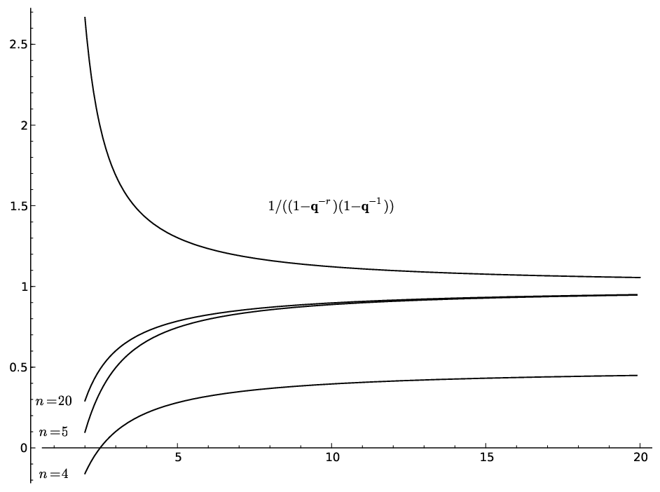
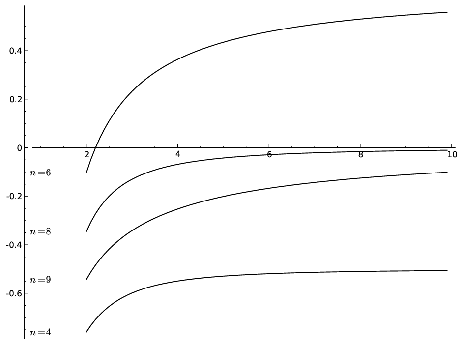
Figure 2: The normalized relative error in Theorem 3.41 for r=2r=2.

Figure 2shows plots of (𝖱n​(𝐪)−ρr,n​(𝐪))/(ρr,n​(𝐪)​𝐪−(r+n−2r−1)+r⁡(r+1)/2)({\mathsf{R}_{n}}(\mathbf{q})-\rho_{r,n}(\mathbf{q}))/(\rho_{r,n}(\mathbf{q})\mathbf{q}^{-\binom{r+n-2}{r-1}+r(r+1)/2}) for r=2r=2 and n=4,5,20n=4,5,20 as we substitute for 𝐪\mathbf{q} real numbers from 22 to 2020. Theorem 4.4 says that the values are absolutely at most 1/((1−𝐪−r)​(1−𝐪−1))1/((1-\mathbf{q}^{-r})(1-\mathbf{q}^{-1})). Theorem 3.41 indicates a bound of 1/2+o⁡(1)1/2+o(1) for n=4n=4 and 1+o⁡(1)1+o(1) for n>4n>4, but without explicit error estimate.

According to (4.10), the bound on the absolute value of the relative error for n≥4n\geq 4 is

q−br−1,n−1+br−1,2(1−q−1)​(1−q−r).\frac{q^{-b_{r-1,n-1}+b_{r-1,2}}}{(1-q^{-1})(1-q^{-r})}. (4.31)

For n>4n>4, this is at most 2/32/3. For n=4n=4, we can drop the factor 1−q−11-q^{-1}, since the sum in (4.18) consists only of a single summand and the estimate by a geometric sum is not necessary. This shows that also for n=4n=4, the relative error is at most 2/32/3.

4.32.

How close is our relative error estimate to being exponentially decaying in the input size? The usual dense representation of a polynomial in rr variables and of degree nn requires br,n=(r+nr)b_{r,n}=\binom{r+n}{r} monomials, each of them equipped with a coefficient from 𝔽q\mathbb{F}_{q}, using about log2⁡q\log_{2}q bits. Thus the total input size is about log2⁡q⋅br,n\log_{2}q\cdot b_{r,n} bits. This differs from log2⁡q⋅(br−1,n−1−br−1,2)\log_{2}q\cdot(b_{r-1,n-1}-b_{r-1,2}) by a factor of

br,nbr−1,n−1−br−1,2<br,n12​br−1,n−1=2​(n+r)​(n+r−1)n​r.\frac{b_{r,n}}{b_{r-1,n-1}-b_{r-1,2}}<\frac{b_{r,n}}{\frac{1}{2}b_{r-1,n-1}}=\frac{2(n+r)(n+r-1)}{nr}.

Up to this polynomial difference (in the exponent), the relative error is exponentially decaying in the bit size of the input, that is, (log⁡q)(\log q) times the number of coefficients in the usual dense representation. In particular, it is exponentially decaying in any of the parameters rr, nn, and log2⁡q\log_{2}q, when the other two are fixed.

These bounds fit well into the picture described in Section 2 of von zur Gathen (2008) for r=2r=2. The family of functions described there approximates the quotient #​R2,n/#​P2,n\#R_{2,n}/\#P_{2,n} (using our notation). If we compare them to ρr,2​(q)/#​P2,n\rho_{r,2}(q)/\#P_{2,n} we find that they differ only by the factor 1−q−n−11-q^{-n-1}, which tends to 11 as nn and qq increase. Our bound 3​q−n+33q^{-n+3} on the relative error for r=2r=2 and n≥4n\geq 4 is only slightly larger than the bound 2​q−n+32q^{-n+3} in Theorem 2.1(ii) of the paper cited.

The following provides some handy bounds.

4.33.

For r,q≥2r,q\geq 2, and n≥5n\geq 5, we have

14​q(r+n−1r)+r−1≤#​Rr,n​(𝔽q)≤6​q(r+n−1r)+r−1,\displaystyle\frac{1}{4}q^{\binom{r+n-1}{r}+r-1}\leq\#R_{r,n}(\mathbb{F}_{q})\leq 6q^{\binom{r+n-1}{r}+r-1}, (4.34)
14​q−(r+n−1r−1)+r≤#​Rr,n​(𝔽q)#​Pr,n​(𝔽q)≤3​q−(r+n−1r−1)+r.\displaystyle\frac{1}{4}q^{-\binom{r+n-1}{r-1}+r}\leq\frac{\#R_{r,n}(\mathbb{F}_{q})}{\#P_{r,n}(\mathbb{F}_{q})}\leq 3q^{-\binom{r+n-1}{r-1}+r}. (4.35)

We conclude this section with bounds for the number of irreducible polynomials.

4.36.

Let r,q≥2r,q\geq 2, and ρr,n\rho_{r,n} as in Theorem 3.41. We have

#​Pr,n​(𝔽q)−2​ρr,n​(q)≤#​Ir,n​(𝔽q)≤#​Pr,n​(𝔽q),\#P_{r,n}(\mathbb{F}_{q})-2\rho_{r,n}(q)\leq\#I_{r,n}(\mathbb{F}_{q})\leq\#P_{r,n}(\mathbb{F}_{q}), (4.37)

and more precisely

#​Ir,1​(𝔽q)\displaystyle\#I_{r,1}(\mathbb{F}_{q}) =#​Pr,1​(𝔽q),\displaystyle=\#P_{r,1}(\mathbb{F}_{q}),
#​Ir,2​(𝔽q)\displaystyle\#I_{r,2}(\mathbb{F}_{q}) =#​Pr,2​(𝔽q)−ρr,2​(q)2⋅(1−q−r−1),\displaystyle=\#P_{r,2}(\mathbb{F}_{q})-\frac{\rho_{r,2}(q)}{2}\cdot(1-q^{-r-1}),
|#​Ir,3​(𝔽q)−(#​Pr,3​(𝔽q)−ρr,3​(q))|\displaystyle\left|\#I_{r,3}(\mathbb{F}_{q})-(\#P_{r,3}(\mathbb{F}_{q})-\rho_{r,3}(q))\right| ≤ρr,3(q)⋅q−(r−1)r/2,\displaystyle\leq\rho_{r,3}(q)\cdot q^{-(r-1)r/2},
and for n≥4n\geq 4
|#​Ir,n​(𝔽q)−(#​Pr,n​(𝔽q)−ρr,n​(q))|\displaystyle\left|\#I_{r,n}(\mathbb{F}_{q})-(\#P_{r,n}(\mathbb{F}_{q})-\rho_{r,n}(q))\right| ≤ρr,n​(q)⋅3​q−(r+n−2r−1)+r⁡(r+1)/2.\displaystyle\leq\rho_{r,n}(q)\cdot 3q^{-\binom{r+n-2}{r-1}+r(r+1)/2}.
Proof.

The more precise statements follow directly from Theorem 4.4 by application of #​Pr,n​(𝔽q)=#​Rr,n​(𝔽q)+#​Ir,n​(𝔽q)\#P_{r,n}(\mathbb{F}_{q})=\#R_{r,n}(\mathbb{F}_{q})+\#I_{r,n}(\mathbb{F}_{q}). These imply the first claim for n<4n<4. For n≥4n\geq 4, the relative error in (4.10) is at most 2/3<12/3<1 as remarked after the proof of Theorem 4.4 and this concludes the proof of (4.37). ∎

5 Powerful polynomials

For an integer s≥2s\geq 2, a polynomial is called ss-powerful if it is divisible by the ssth power of some nonconstant polynomial, and ss-powerfree otherwise; it is squarefree if s=2s=2. Let

Qr,n,s​(F)\displaystyle Q_{r,n,s}(F) ={f∈Pr,n(F):f is s-powerful},\displaystyle=\{f\in P_{r,n}(F)\colon f\text{ is $s$-powerful}\},
Sr,n,s​(F)\displaystyle S_{r,n,s}(F) =Pr,n​(F)∖Qr,n,s​(F).\displaystyle=P_{r,n}(F)\setminus Q_{r,n,s}(F).

As in the previous section, we restrict our attention to a finite field F=𝔽qF=\mathbb{F}_{q}, which we omit from the notation.

For the approach by generating functions, we consider the combinatorial classes 𝒬=⋃n≥0Qr,n,s{\mathcal{Q}}=\bigcup_{n\geq 0}Q_{r,n,s} and 𝒮=𝒫∖𝒬{\mathcal{S}}={\mathcal{P}}\setminus{\mathcal{Q}}, where the explicit reference to rr and ss is omitted. Any monic polynomial ff factors uniquely as f=g⋅hsf=g\cdot h^{s} where gg is a monic ss-powerfree polynomial and hh an arbitrary monic polynomial, hence

P=S⋅P⁡(zs){\mathrm{P}}={\mathrm{S}}\cdot{\mathrm{P}}(z^{s}) (5.1)

and by definition Q=P−S{\mathrm{Q}}={\mathrm{P}}-{\mathrm{S}} for the generating functions of 𝒮{\mathcal{S}} and 𝒬{\mathcal{Q}}, respectively. For univariate polynomials, Carlitz (1932) derives (5.1) directly from generating functions to prove the counting formula which we reproduce in (5.10). Flajolet et al. (2001, Section 1.1) use (5.1) for s=2s=2 to count univariate squarefree polynomials, see also Flajolet & Sedgewick (2009, Note I.66). A corresponding Maple program to compute the coefficients of Q{\mathrm{Q}} is shown in Figure 3. It was used to compute #​Q2,n,2​(𝔽q)\#Q_{2,n,2}(\mathbb{F}_{q}) for n≤6n\leq 6 in von zur Gathen (2008, Table 3.1). We extend this in Table 3.

spowerfreesGF:=proc(z,N,r,s) local i: option remember: convert(taylor(allpolysGF(z,N,r)/allpolysGF(zˆs,N,r), z,N+1),polynom):end:spowerfulsGF:=proc(z,N,r,s) option remember: allpolysGF(z,N,r)-spowerfreesGF(z,N,r,s):end:spowerfuls:=proc(n,r,s) coeff(sort(expand(spowerfulsGF(z,n,r,s))),zˆn):end:

Figure 3: Maple program to compute the number of monic ss-powerful polynomials in rr variables of degree nn.

Table 3: Exact values of #​Qr,n,s​(𝔽q)\#Q_{r,n,s}(\mathbb{F}_{q}) for small values of r,n,sr,n,s.

As in Theorem 3.11, this approach quickly leads to explicit formulas.

5.2.

For r≥1r\geq 1, q,s≥2q,s\geq 2, Pn{\mathrm{P}}_{n} as in (3.4), and MnM_{n} as in (3.10), we have

Sn\displaystyle{\mathrm{S}}_{n} =∑0≤i≤n/sj∈Mi(−1)|j|Pj1Pj2⋯Pj|j|Pn−i​s,\displaystyle=\sum_{\begin{subarray}{c}0\leq i\leq n/s\\ j\in M_{i}\end{subarray}}(-1)^{\lvert j\rvert}{\mathrm{P}}_{j_{1}}{\mathrm{P}}_{j_{2}}\cdots{\mathrm{P}}_{j_{\lvert j\rvert}}{\mathrm{P}}_{n-is}, (5.3)
Qn\displaystyle{\mathrm{Q}}_{n} =−∑1≤i≤n/sj∈Mi(−1)|j|Pj1Pj2⋯Pj|j|Pn−i​s.\displaystyle=-\sum_{\begin{subarray}{c}1\leq i\leq n/s\\ j\in M_{i}\end{subarray}}(-1)^{\lvert j\rvert}{\mathrm{P}}_{j_{1}}{\mathrm{P}}_{j_{2}}\cdots{\mathrm{P}}_{j_{\lvert j\rvert}}{\mathrm{P}}_{n-is}. (5.4)
Proof.

We consider the original power series F=1−P=−∑i≥1Pizi{\mathrm{F}}=1-{\mathrm{P}}=-\sum_{i\geq 1}{\mathrm{P}}_{i}z^{i} and express (5.1) as

S\displaystyle{\mathrm{S}} =P⋅∑i≥0F​(zs)i\displaystyle={\mathrm{P}}\cdot\sum_{i\geq 0}{\mathrm{F}}(z^{s})^{i} (5.5)
=∑k≥0Pkzk⋅∑i≥0(−∑j≥1Pjzj​s)i.\displaystyle=\sum_{k\geq 0}{\mathrm{P}}_{k}z^{k}\cdot\sum_{i\geq 0}\Bigl(-\sum_{j\geq 1}{\mathrm{P}}_{j}z^{js}\Bigr)^{i}. (5.6)

Comparison of coefficients provides us with

Sn\displaystyle{\mathrm{S}}_{n} =∑0≤i≤n/sj∈Mi(−1)|j|Pj1Pj2⋯Pj|j|Pn−i​s,\displaystyle=\sum_{\begin{subarray}{c}0\leq i\leq n/s\\ j\in M_{i}\end{subarray}}(-1)^{\lvert j\rvert}{\mathrm{P}}_{j_{1}}{\mathrm{P}}_{j_{2}}\cdots{\mathrm{P}}_{j_{\lvert j\rvert}}{\mathrm{P}}_{n-is}, (5.7)

and the claim for Qn=Pn−Sn{\mathrm{Q}}_{n}={\mathrm{P}}_{n}-{\mathrm{S}}_{n} follows. ∎

For r=1r=1, we have Pj=qj{\mathrm{P}}_{j}=q^{j} and for any composition j1+j2+⋯+jkj_{1}+j_{2}+\dots+j_{k} of ii in (5.4)

Pj1Pj2⋯PjkPn−i​s=qn−(s−1)​i.{\mathrm{P}}_{j_{1}}{\mathrm{P}}_{j_{2}}\cdots{\mathrm{P}}_{j_{k}}{\mathrm{P}}_{n-is}=q^{n-(s-1)i}. (5.8)

Moreover, since

∑k≥1(−1)k​(i−1k−1)=−(0i−1)={−1if i=1,0if i≥2,\sum_{k\geq 1}(-1)^{k}\binom{i-1}{k-1}=-\binom{0}{i-1}=\begin{cases}-1&\text{if $i=1$},\\ 0&\text{if $i\geq 2$},\end{cases} (5.9)

see Graham et al. (1989, p. 167), we have in the univariate case

Qn=−∑1≤i≤n/sk≥1(−1)k(i−1k−1)qn−(s−1)​i={0if n<s,qn−s+1if n≥s,{\mathrm{Q}}_{n}=-\sum_{\begin{subarray}{c}1\leq i\leq n/s\\ k\geq 1\end{subarray}}(-1)^{k}\binom{i-1}{k-1}q^{n-(s-1)i}=\begin{cases}0&\text{if $n<s$},\\ q^{n-s+1}&\text{if $n\geq s$},\end{cases} (5.10)

as shown by Carlitz (1932, Section 6).

To study the asymptotic behavior of Sn{\mathrm{S}}_{n} and Qn{\mathrm{Q}}_{n} for r≥2r\geq 2 we again deviate from the standard approach and move to power series in ℚ⁡(𝐪)​⟦z⟧\mathbb{Q}(\mathbf{q})\left\llbracket z\right\rrbracket. With 𝖯{\mathsf{P}} from (3.24), we define 𝖲,𝖰∈ℚ⁡(𝐪)​⟦z⟧{\mathsf{S}},{\mathsf{Q}}\in\mathbb{Q}(\mathbf{q})\left\llbracket z\right\rrbracket by

𝖯\displaystyle{\mathsf{P}} =𝖲⋅𝖯⁡(zs),\displaystyle={\mathsf{S}}\cdot{\mathsf{P}}(z^{s}), (5.11)
𝖰\displaystyle{\mathsf{Q}} =𝖯−𝖲.\displaystyle={\mathsf{P}}-{\mathsf{S}}. (5.12)

This is well-defined, since 𝖯⁡(zs){\mathsf{P}}(z^{s}) has constant term 1 and is therefore invertible. By construction, we have

𝖲n​(q)=#​Sr,n,s​(𝔽q),𝖰n​(q)=#​Qr,n,s​(𝔽q).\begin{split}{\mathsf{S}}_{n}(q)&=\#S_{r,n,s}(\mathbb{F}_{q}),\\ {\mathsf{Q}}_{n}(q)&=\#Q_{r,n,s}(\mathbb{F}_{q}).\end{split} (5.13)

To study the asymptotic behavior, we examine 𝖯k⋅𝖯n−s​k{\mathsf{P}}_{k}\cdot{\mathsf{P}}_{n-sk}. Let

vr,n,s​(k)\displaystyle v_{r,n,s}(k) =deg𝐪⁡(𝖯k⋅𝖯n−s​k)\displaystyle=\deg_{\mathbf{q}}({\mathsf{P}}_{k}\cdot{\mathsf{P}}_{n-sk}) (5.14)
=(r+k)r¯/r!+(r+n−s​k)r¯/r!−2\displaystyle=(r+k)^{\underline{r}}/r!+(r+n-sk)^{\underline{r}}/r!-2 (5.15)

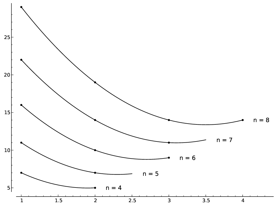
and consider vr,n,s​(k)v_{r,n,s}(k) as a function of a real variable kk (Figure 4). In contrast to u⁡(k)u(k) from Section 3, this function is not monotone in kk.

Refer to caption
Figure 4: Graphs of v2,n,2​(k)v_{2,n,2}(k) on [1,n/2][1,n/2] as nn runs from 44 to 88. The dots represent the values at integer arguments.
5.16.

Let r,n,s,q≥2r,n,s,q\geq 2.

  1. (i)

    The function vr,n,s​(k)v_{r,n,s}(k) is convex for 1≤k≤n/s1\leq k\leq n/s.

  2. (ii)

    For all integers kk with 2≤k≤n/s2\leq k\leq n/s, we have

    vr,n,s​(1)>vr,n,s​(k).v_{r,n,s}(1)>v_{r,n,s}(k).
  3. (iii)

    For all integers kk with 3≤k≤n/s3\leq k\leq n/s, we have

    vr,n,s​(2)\displaystyle v_{r,n,s}(2) >vr,n,s​(k)\displaystyle>v_{r,n,s}(k) if (n,s)≠(6,2).\displaystyle\text{if $(n,s)\neq(6,2)$}. (5.17)
    Furthermore,
    vr,6,2​(2)\displaystyle v_{r,6,2}(2) <vr,6,2​(3)\displaystyle<v_{r,6,2}(3) if r≥3,\displaystyle\text{if $r\geq 3$}, (5.18)
    v2,6,2​(2)\displaystyle v_{2,6,2}(2) =v2,6,2​(3)+1.\displaystyle=v_{2,6,2}(3)+1. (5.19)
  4. (iv)

    If (n,s)≠(6,2)(n,s)\neq(6,2), then

    ∑2≤k≤n/sqvr,n,s​(k)≤2​qvr,n,s​(2)1−q−1.\sum_{2\leq k\leq n/s}q^{v_{r,n,s}(k)}\leq\frac{2q^{v_{r,n,s}(2)}}{1-q^{-1}}. (5.20)
Proof.

We switch to the affine transformation

v¯​(k)\displaystyle\bar{v}(k) =r!⋅(vr,n,s​(k)+2)\displaystyle=r!\cdot\Bigl(v_{r,n,s}(k)+2\Bigr) (5.21)
=(r+k)r¯+(r+n−s​k)r¯,\displaystyle=(r+k)^{\underline{r}}+(r+n-sk)^{\underline{r}}, (5.22)

which exhibits the same behavior as vr,n,sv_{r,n,s} concerning convexity and maximality.

  1. (i)

    We have

    v¯′′​(k)=∑1≤i,j≤ri≠j((r+k)r¯(i+k)​(j+k)+s2​(r+n−s​k)r¯(i+n−s​k)​(j+n−s​k))>0.\bar{v}^{\prime\prime}(k)=\sum_{\begin{subarray}{c}1\leq i,j\leq r\\ i\neq j\end{subarray}}\Bigl(\frac{(r+k)^{\underline{r}}}{(i+k)(j+k)}+\frac{s^{2}(r+n-sk)^{\underline{r}}}{(i+n-sk)(j+n-sk)}\Bigr)>0. (5.23)
  2. (ii)

    For n<2​sn<2s, there is nothing to prove. For n≥2​sn\geq 2s, we find n≥s+2≥s+1+1/(s−1)n\geq s+2\geq s+1+1/(s-1) and for all ii

    (i+n−s)−(i+n/s)≥0,\displaystyle(i+n-s)-(i+n/s)\geq 0, (5.24)
    (r+n−s)r¯−(r+n/s)r¯≥0,\displaystyle(r+n-s)^{\underline{r}}-(r+n/s)^{\underline{r}}\geq 0, (5.25)
    v¯​(1)−v¯​(n/s)\displaystyle\bar{v}(1)-\bar{v}(n/s) =(r+1)!+(r+n−s)r¯−(r+n/s)r¯−r!\displaystyle=(r+1)!+(r+n-s)^{\underline{r}}-(r+n/s)^{\underline{r}}-r! (5.26)
    =(r+n−s)r¯−(r+n/s)r¯+r⋅r!>0.\displaystyle=(r+n-s)^{\underline{r}}-(r+n/s)^{\underline{r}}+r\cdot r!>0. (5.27)

    With the convexity of v¯\bar{v}, this suffices.

  3. (iii)

    Analogously to (ii), it is sufficient to prove v¯​(2)>v¯​(n/s)\bar{v}(2)>\bar{v}(n/s) for (n,s)≠(6,2)(n,s)\neq(6,2). If n≥2​s2/(s−1)n\geq 2s^{2}/(s-1), then n−2​s≥n/sn-2s\geq n/s, so that for all ii

    (i+n−2​s)−(i+n/s)≥0(i+n-2s)-(i+n/s)\geq 0

    and hence

    v¯​(2)−v¯​(n/s)\displaystyle\bar{v}(2)-\bar{v}(n/s) =(r+2)!/2+(r+n−2​s)r¯−(r+n/s)r¯−r!\displaystyle=(r+2)!/2+(r+n-2s)^{\underline{r}}-(r+n/s)^{\underline{r}}-r!
    >(r+n−2​s)r¯−(r+n/s)r¯≥0.\displaystyle>(r+n-2s)^{\underline{r}}-(r+n/s)^{\underline{r}}\geq 0.

    If n<2​s2/(s−1)n<2s^{2}/(s-1), then n/s<3n/s<3 for s≥3s\geq 3 or n<6n<6 and there is nothing to prove. Finally, the three conditions n<2​s2/(s−1)n<2s^{2}/(s-1), s=2s=2, and n≥6n\geq 6 enforce 6≤n<86\leq n<8, and we compute directly

    vr,7,2​(2)−vr,7,2​(3)=12​r​(r+1)>0,v_{r,7,2}(2)-v_{r,7,2}(3)=\frac{1}{2}r(r+1)>0,
    vr,6,2​(2)−vr,6,2​(3)=−16​(r−3)​(r+1)​(r+2)−1​{=1 if ​r=2,<0 if ​r≥3.v_{r,6,2}(2)-v_{r,6,2}(3)=-\frac{1}{6}(r-3)(r+1)(r+2)-1\begin{cases}=1&\text{ if }r=2,\\ <0&\text{ if }r\geq 3.\end{cases}
  4. (iv)

    The maximal value of the integer sequence vr,n,s​(k)v_{r,n,s}(k) for 2≤k≤n/s2\leq k\leq n/s is vr,n,s​(2)v_{r,n,s}(2) by (iii). Each value is taken at most twice, due to (i), and we can bound the sum by twice a geometric sum as

    ∑2≤k≤n/sqvr,n,s​(k)≤2​qvr,n,s​(2)​∑k≥0q−k=2​qvr,n,s​(2)1−q−1.∎\sum_{2\leq k\leq n/s}q^{v_{r,n,s}(k)}\leq 2q^{v_{r,n,s}(2)}\sum_{k\geq 0}q^{-k}=\frac{2q^{v_{r,n,s}(2)}}{1-q^{-1}}.\mbox{\qed} (5.28)

The approach by generating functions now yields the following result. Its “general” case is (iv). We give exact expressions in special cases, namely for n<3​sn<3s in (ii) and for (n,s)=(6,2)(n,s)=(6,2) in (iii), which also apply when we substitute the size qq of a finite field 𝔽q\mathbb{F}_{q} for 𝐪\mathbf{q}.

5.29.

Let r,s≥2r,s\geq 2, n≥0n\geq 0, and

ηr,n,s​(𝐪)\displaystyle\eta_{r,n,s}(\mathbf{q}) =𝐪(r+n−sr)+r−1​(1−𝐪−r)​(1−𝐪−(r+n−s−1r−1))(1−𝐪−1)2∈ℚ⁡(𝐪),\displaystyle=\mathbf{q}^{\binom{r+n-s}{r}+r-1}\frac{(1-\mathbf{q}^{-r})(1-\mathbf{q}^{-\binom{r+n-s-1}{r-1}})}{(1-\mathbf{q}^{-1})^{2}}\in\mathbb{Q}(\mathbf{q}), (5.30)
δ\displaystyle\delta =(r+n−sr)−(r+n−2​sr)−r⁡(r+1)2.\displaystyle=\binom{r+n-s}{r}-\binom{r+n-2s}{r}-\frac{r(r+1)}{2}. (5.31)
  1. (i)

    If n≥2​sn\geq 2s, then δ≥r\delta\geq r.

  2. (ii)
    𝖰n={0for n<s,ηr,n,s​(𝐪)for s≤n<2​s,ηr,n,s​(𝐪)​(1+𝐪−δ⋅1−𝐪−(n+r−2​s−1r−1)1−𝐪−(n+r−s−1r−1)CLOSE⋅(1−𝐪−r(r+1)/21−𝐪−r−𝐪−r(r−1)/21−𝐪−r1−𝐪−1))for 2​s≤n<3​s.{\mathsf{Q}}_{n}=\begin{cases}0&\text{for $n<s$,}\\ \eta_{r,n,s}(\mathbf{q})&\text{for $s\leq n<2s$,}\\ \eta_{r,n,s}(\mathbf{q})\biggl(1+\mathbf{q}^{-\delta}\cdot\frac{1-\mathbf{q}^{-\binom{n+r-2s-1}{r-1}}}{1-\mathbf{q}^{-\binom{n+r-s-1}{r-1}}}&\\ \quad\cdot\Bigl(\frac{1-\mathbf{q}^{-r(r+1)/2}}{1-\mathbf{q}^{-r}}-\mathbf{q}^{-r(r-1)/2}\frac{1-\mathbf{q}^{-r}}{1-\mathbf{q}^{-1}}\Bigr)\biggr)&\text{for $2s\leq n<3s$.}\end{cases} (5.32)
  3. (iii)

    For (n,s)=(6,2)(n,s)=(6,2) and r≥2r\geq 2, we have

    𝖰6\displaystyle{\mathsf{Q}}_{6} =ηr,6,2​(𝐪)​(1+𝐪−(r+34)−r+1⋅(𝐪−1​(1−𝐪−1)​(1−𝐪−(r+23))(1−𝐪−r)​(1−𝐪−(r+34))CLOSECLOSE\displaystyle=\eta_{r,6,2}(\mathbf{q})\bigg(1+\mathbf{q}^{-\binom{r+3}{4}-r+1}\cdot\Big(\mathbf{q}^{-1}\tfrac{(1-\mathbf{q}^{-1})\bigl(1-\mathbf{q}^{-\binom{r+2}{3}}\bigr)}{(1-\mathbf{q}^{-r})\bigl(1-\mathbf{q}^{-\binom{r+3}{4}}\bigr)} (5.33)
    +𝐪−(r3−7r+6)/6(1−𝐪−r(r+1)/2)2(1−𝐪−r)​(1−𝐪−(r+34))\displaystyle\quad+\mathbf{q}^{-(r^{3}-7r+6)/6}\tfrac{(1-\mathbf{q}^{-r(r+1)/2})^{2}}{(1-\mathbf{q}^{-r})\bigl(1-\mathbf{q}^{-\binom{r+3}{4}}\bigr)} (5.34)
    −𝐪−(r3+3r2−10r+6)/6(1−𝐪−r)(1−𝐪−r(r+1)/2)(1−𝐪−1)​(1−𝐪−(r+34))\displaystyle\quad-\mathbf{q}^{-(r^{3}+3r^{2}-10r+6)/6}\tfrac{(1-\mathbf{q}^{-r})(1-\mathbf{q}^{-r(r+1)/2})}{(1-\mathbf{q}^{-1})\bigl(1-\mathbf{q}^{-\binom{r+3}{4}}\bigr)} (5.35)
    −2𝐪−(r3+3r2+4r−6)/61−𝐪−r(r+1)/21−𝐪−(r+34)\displaystyle\quad-2\mathbf{q}^{-(r^{3}+3r^{2}+4r-6)/6}\tfrac{1-\mathbf{q}^{-r(r+1)/2}}{1-\mathbf{q}^{-\binom{r+3}{4}}} (5.36)
    +𝐪−(r3+6r2−7r+6)/6(1−𝐪−r)2(1−𝐪−1)​(1−𝐪−(r+34))))\displaystyle\quad+\mathbf{q}^{-(r^{3}+6r^{2}-7r+6)/6}\tfrac{(1-\mathbf{q}^{-r})^{2}}{(1-\mathbf{q}^{-1})\big(1-\mathbf{q}^{-\binom{r+3}{4}}\big)}\Big)\bigg) (5.37)
    =ηr,6,2​(𝐪)​(1+𝐪−δ+(r−2)​(r−1)​(r+3)/6​(1+O⁡(𝐪−1))).\displaystyle=\eta_{r,6,2}(\mathbf{q})\bigl(1+\mathbf{q}^{-\delta+(r-2)(r-1)(r+3)/6}(1+O(\mathbf{q}^{-1}))\bigr). (5.38)
  4. (iv)

    For n≥2​sn\geq 2s and (n,s)≠(6,2)(n,s)\neq(6,2), we have

    𝖰n=ηr,n,s​(𝐪)​(1+𝐪−δ​(1+O⁡(𝐪−1))).{\mathsf{Q}}_{n}=\eta_{r,n,s}(\mathbf{q})\big(1+\mathbf{q}^{-\delta}(1+O(\mathbf{q}^{-1}))\big). (5.39)
Proof.
  1. (i)

    If n≥2​sn\geq 2s, then

    δ≥(r+sr)−1−r⁡(r+1)2≥(r+2r)−1−r⁡(r+1)2=r.\delta\geq\binom{r+s}{r}-1-\frac{r(r+1)}{2}\geq\binom{r+2}{r}-1-\frac{r(r+1)}{2}=r. (5.40)
  2. (ii)

    The exact formulas of Theorem 5.2 yield

    𝖰n\displaystyle{\mathsf{Q}_{n}} =0\displaystyle=0 for n<s,\displaystyle\text{for $n<s$}, (5.41)
    𝖰n\displaystyle{\mathsf{Q}_{n}} =𝖯1​𝖯n−s=ηr,n,s​(𝐪)\displaystyle={\mathsf{P}}_{1}{\mathsf{P}}_{n-s}=\eta_{r,n,s}(\mathbf{q}) for s≤n<2​s,\displaystyle\text{for $s\leq n<2s$}, (5.42)

    and for 2​s≤n<3​s2s\leq n<3s,

    𝖲n\displaystyle{\mathsf{S}}_{n} =𝖯n−𝖯1​𝖯n−s−(𝖯2−𝖯12)​𝖯n−2​s,\displaystyle={\mathsf{P}}_{n}-{\mathsf{P}}_{1}{\mathsf{P}}_{n-s}-({\mathsf{P}}_{2}-{\mathsf{P}}_{1}^{2}){\mathsf{P}}_{n-2s}, (5.43)
    𝖰n\displaystyle{\mathsf{Q}}_{n} =𝖯1​𝖯n−s+(𝖯2−𝖯12)​𝖯n−2​s\displaystyle={\mathsf{P}}_{1}{\mathsf{P}}_{n-s}+({\mathsf{P}}_{2}-{\mathsf{P}}_{1}^{2}){\mathsf{P}}_{n-2s} (5.44)
    =ηr,n,s​(𝐪)​(1+𝖯2​𝖯n−2​s𝖯1​𝖯n−s​(1−𝖯12𝖯2))\displaystyle=\eta_{r,n,s}(\mathbf{q})\Bigl(1+\frac{{\mathsf{P}}_{2}{\mathsf{P}}_{n-2s}}{{\mathsf{P}}_{1}{\mathsf{P}}_{n-s}}\Bigl(1-\frac{{\mathsf{P}}_{1}^{2}}{{\mathsf{P}}_{2}}\Bigr)\Bigr) (5.45)
    =ηr,n,s​(𝐪)​(1+𝐪−δ​1−𝐪−(n+r−2​s−1r−1)1−𝐪−(n+r−s−1r−1)CLOSE\displaystyle=\eta_{r,n,s}(\mathbf{q})\bigg(1+\mathbf{q}^{-\delta}\frac{1-\mathbf{q}^{-\binom{n+r-2s-1}{r-1}}}{1-\mathbf{q}^{-\binom{n+r-s-1}{r-1}}} (5.46)
    ⋅(1−𝐪−r(r+1)/21−𝐪−r−𝐪−r(r−1)/21−𝐪−r1−𝐪−1)),\displaystyle\quad\quad\cdot\Big(\frac{1-\mathbf{q}^{-r(r+1)/2}}{1-\mathbf{q}^{-r}}-\mathbf{q}^{-r(r-1)/2}\frac{1-\mathbf{q}^{-r}}{1-\mathbf{q}^{-1}}\Big)\bigg), (5.47)

    where δ=−deg𝐪⁡(𝖯2​𝖯n−2​s/(𝖯1​𝖯n−s))\delta=-\deg_{\mathbf{q}}({\mathsf{P}}_{2}{\mathsf{P}}_{n-2s}/({\mathsf{P}}_{1}{\mathsf{P}}_{n-s})).

  3. (iii)

    For s=2s=2, we evaluate (5.4) for

    𝖰6\displaystyle{\mathsf{Q}}_{6} =𝖯1​𝖯4+𝖯3+𝖯22−𝖯12​𝖯2−2​𝖯1​𝖯2+𝖯13\displaystyle={\mathsf{P}}_{1}{\mathsf{P}}_{4}+{\mathsf{P}}_{3}+{\mathsf{P}}_{2}^{2}-{\mathsf{P}}_{1}^{2}{\mathsf{P}}_{2}-2{\mathsf{P}}_{1}{\mathsf{P}}_{2}+{\mathsf{P}}_{1}^{3} (5.48)
    =ηr,6,2​(𝐪)​(1+(𝖯3+𝖯22−𝖯12​𝖯2−2​𝖯1​𝖯2+𝖯13)/(𝖯1​𝖯4))\displaystyle=\eta_{r,6,2}(\mathbf{q})(1+({\mathsf{P}}_{3}+{\mathsf{P}}_{2}^{2}-{\mathsf{P}}_{1}^{2}{\mathsf{P}}_{2}-2{\mathsf{P}}_{1}{\mathsf{P}}_{2}+{\mathsf{P}}_{1}^{3})/({\mathsf{P}}_{1}{\mathsf{P}}_{4})) (5.49)
    =ηr,6,2​(𝐪)​(1+𝐪−vr,6,2​(1)+vr,6,2​(3)+1CLOSE\displaystyle=\eta_{r,6,2}(\mathbf{q})\biggl(1+\mathbf{q}^{-v_{r,6,2}(1)+v_{r,6,2}(3)+1} (5.50)
    ⋅(𝐪−1​(1−𝐪−1)​(1−𝐪−br−1,3)(1−𝐪−r)​(1−𝐪−br−1,4)CLOSE\displaystyle\quad\cdot\Bigl(\mathbf{q}^{-1}\tfrac{(1-\mathbf{q}^{-1})(1-\mathbf{q}^{-b_{r-1,3}})}{(1-\mathbf{q}^{-r})(1-\mathbf{q}^{-b_{r-1,4}})} (5.51)
    +𝐪−(r3−7r+6)/6(1−𝐪−r(r+1)/2)2(1−𝐪−r)​(1−𝐪−br−1,4)\displaystyle\quad+\mathbf{q}^{-(r^{3}-7r+6)/6}\tfrac{(1-\mathbf{q}^{-r(r+1)/2})^{2}}{(1-\mathbf{q}^{-r})(1-\mathbf{q}^{-b_{r-1,4}})} (5.52)
    −𝐪−(r3+3r2−10r+6)/6(1−𝐪−r)(1−𝐪−r(r+1)/2)(1−𝐪−1)​(1−𝐪−br−1,4)\displaystyle\quad-\mathbf{q}^{-(r^{3}+3r^{2}-10r+6)/6}\tfrac{(1-\mathbf{q}^{-r})(1-\mathbf{q}^{-r(r+1)/2})}{(1-\mathbf{q}^{-1})(1-\mathbf{q}^{-b_{r-1,4}})} (5.53)
    −2𝐪−(r3+3r2+4r−6)/61−𝐪−r(r+1)/21−𝐪−br−1,4\displaystyle\quad-2\mathbf{q}^{-(r^{3}+3r^{2}+4r-6)/6}\tfrac{1-\mathbf{q}^{-r(r+1)/2}}{1-\mathbf{q}^{-b_{r-1,4}}} (5.54)
    +𝐪−(r3+6r2−7r+6)/6(1−𝐪−r)2(1−𝐪−1)​(1−𝐪−br−1,4)))\displaystyle\quad+\mathbf{q}^{-(r^{3}+6r^{2}-7r+6)/6}\tfrac{(1-\mathbf{q}^{-r})^{2}}{(1-\mathbf{q}^{-1})(1-\mathbf{q}^{-b_{r-1,4}})}\Bigr)\biggr) (5.55)
    =ηr,6,2​(𝐪)​(1+𝐪−δ+(r−2)​(r−1)​(r+3)/6​(1+O⁡(𝐪−1))),\displaystyle=\eta_{r,6,2}(\mathbf{q})\big(1+\mathbf{q}^{-\delta+(r-2)(r-1)(r+3)/6}(1+O(\mathbf{q}^{-1}))\big), (5.56)

    since the sum (5.51)–(5.55) has nonpositive degree in 𝐪\mathbf{q} and −vr,6,2​(1)+vr,6,2​(3)+1=−(r+34)−r+1=−δ+(r−2)​(r−1)​(r+3)/6-v_{r,6,2}(1)+v_{r,6,2}(3)+1=-\binom{r+3}{4}-r+1=-\delta+(r-2)(r-1)(r+3)/6.

  4. (iv)

    Finally, for n≥2​sn\geq 2s and (n,s)≠(6,2)(n,s)\neq(6,2), we claim

    𝖲n=𝖯n−𝖯1​𝖯n−s−𝖯2​𝖯n−2​s​(1+O⁡(𝐪−1)).{\mathsf{S}}_{n}={\mathsf{P}}_{n}-{\mathsf{P}}_{1}{\mathsf{P}}_{n-s}-{\mathsf{P}}_{2}{\mathsf{P}}_{n-2s}(1+O(\mathbf{q}^{-1})). (5.57)

    This implies immediately

    𝖲n=𝖯n−𝖯1​𝖯n−s​(1+O⁡(𝐪−1))=𝖯n​(1+O⁡(𝐪−1)),\begin{split}{\mathsf{S}}_{n}&={\mathsf{P}}_{n}-{\mathsf{P}}_{1}{\mathsf{P}}_{n-s}(1+O(\mathbf{q}^{-1}))\\ &={\mathsf{P}}_{n}(1+O(\mathbf{q}^{-1})),\end{split} (5.58)

    by Lemmas 5.16 (ii) and 3.30 (i), respectively. We already have (5.57) for 2​s≤n<3​s2s\leq n<3s from (5.43) by 3.30 (i). We also have (5.58) for (n,s)=(6,2)(n,s)=(6,2) from (5.56). This is enough to obtain inductively

    𝖲n\displaystyle{\mathsf{S}}_{n} =𝖯n−∑1≤i≤n/s𝖲n−i​s​𝖯i\displaystyle={\mathsf{P}}_{n}-\sum_{1\leq i\leq n/s}{\mathsf{S}}_{n-is}{\mathsf{P}}_{i} (5.59)
    =𝖯n−𝖯1​𝖲n−s−∑2≤i≤n/s𝖯i​𝖲n−i​s\displaystyle={\mathsf{P}}_{n}-{\mathsf{P}}_{1}{\mathsf{S}}_{n-s}-\sum_{2\leq i\leq n/s}{\mathsf{P}}_{i}{\mathsf{S}}_{n-is} (5.60)
    =𝖯n−𝖯1​(𝖯n−s−𝖯1​𝖯n−2​s​(1+O⁡(𝐪−1)))−∑2≤i≤n/s𝖯i​𝖯n−i​s​(1+O⁡(𝐪−1))\displaystyle={\mathsf{P}}_{n}-{\mathsf{P}}_{1}\bigl({\mathsf{P}}_{n-s}-{\mathsf{P}}_{1}{\mathsf{P}}_{n-2s}(1+O(\mathbf{q}^{-1}))\bigr)-\sum_{2\leq i\leq n/s}{\mathsf{P}}_{i}{\mathsf{P}}_{n-is}(1+O(\mathbf{q}^{-1})) (5.61)
    =𝖯n−𝖯1​𝖯n−s+𝖯12​𝖯n−2​s​(1+O⁡(𝐪−1))−𝖯2​𝖯n−2​s​(1+O⁡(𝐪−1))\displaystyle={\mathsf{P}}_{n}-{\mathsf{P}}_{1}{\mathsf{P}}_{n-s}+{\mathsf{P}}_{1}^{2}{\mathsf{P}}_{n-2s}(1+O(\mathbf{q}^{-1}))-{\mathsf{P}}_{2}{\mathsf{P}}_{n-2s}(1+O(\mathbf{q}^{-1})) (5.62)
    =𝖯n−𝖯1​𝖯n−s−𝖯2​𝖯n−2​s​(1+O⁡(𝐪−1)),\displaystyle={\mathsf{P}}_{n}-{\mathsf{P}}_{1}{\mathsf{P}}_{n-s}-{\mathsf{P}}_{2}{\mathsf{P}}_{n-2s}(1+O(\mathbf{q}^{-1})), (5.63)

    using 5.16 (iii) for (n,s)≠(6,2)(n,s)\neq(6,2) and 3.30 (i). We conclude with

    𝖰n\displaystyle{\mathsf{Q}}_{n} =𝖯1​𝖯n−s+𝖯2​𝖯n−2​s​(1+O⁡(𝐪−1))\displaystyle={\mathsf{P}}_{1}{\mathsf{P}}_{n-s}+{\mathsf{P}}_{2}{\mathsf{P}}_{n-2s}(1+O(\mathbf{q}^{-1})) (5.64)
    =ηr,n,s​(𝐪)​(1+𝐪−δ​(1+O⁡(𝐪−1)))\displaystyle=\eta_{r,n,s}(\mathbf{q})(1+\mathbf{q}^{-\delta}(1+O(\mathbf{q}^{-1}))) (5.65)

    by the definition of ηr,n,s​(𝐪)=𝖯1​𝖯n−s\eta_{r,n,s}(\mathbf{q})={\mathsf{P}}_{1}{\mathsf{P}}_{n-s} and δ=−deg𝐪⁡(𝖯2​𝖯n−2​s/(𝖯1​𝖯n−s))\delta=-\deg_{\mathbf{q}}({\mathsf{P}}_{2}{\mathsf{P}}_{n-2s}/({\mathsf{P}}_{1}{\mathsf{P}}_{n-s})), respectively. ∎

For r≥3r\geq 3, we can replace 1+O⁡(𝐪−1)1+O(\mathbf{q}^{-1}) in (5.38) by 𝐪−1+O⁡(𝐪−2)\mathbf{q}^{-1}+O(\mathbf{q}^{-2}).

In the following, the combinatorial approach replaces the asymptotic 1+O⁡(𝐪−1)1+O(\mathbf{q}^{-1}) of (5.39) with an explicit bound of 66 in (5.72). We consider for integers 1≤k≤n/s1\leq k\leq n/s the sets

Qr,n,s,k(F)={g⋅hs:g∈Pr,n−s​k,h∈Pr,k}∈Pr,n(F)Q_{r,n,s,k}(F)=\{g\cdot h^{s}\colon g\in P_{r,n-sk},h\in P_{r,k}\}\in P_{r,n}(F) (5.66)

and have

Qr,n,s​(F)=⋃1≤k≤n/sQr,n,s,k​(F).Q_{r,n,s}(F)=\bigcup_{1\leq k\leq n/s}Q_{r,n,s,k}(F). (5.67)

For n<3​sn<3s the exact formula (5.32) of Theorem 5.29 (ii) applies. We provide explicit bounds for n≥3​sn\geq 3s.

5.68.

Let r,s,q≥2r,s,q\geq 2, n≥0n\geq 0, and

ηr,n,s​(𝐪)\displaystyle\eta_{r,n,s}(\mathbf{q}) =𝐪(r+n−sr)+r−1​(1−𝐪−r)​(1−𝐪−(r+n−s−1r−1))(1−𝐪−1)2∈ℚ⁡(𝐪),\displaystyle=\mathbf{q}^{\binom{r+n-s}{r}+r-1}\frac{(1-\mathbf{q}^{-r})\bigl(1-\mathbf{q}^{-\binom{r+n-s-1}{r-1}}\bigr)}{(1-\mathbf{q}^{-1})^{2}}\in\mathbb{Q}(\mathbf{q}), (5.69)
δ\displaystyle\delta =(r+n−sr)−(r+n−2​sr)−r⁡(r+1)2\displaystyle=\binom{r+n-s}{r}-\binom{r+n-2s}{r}-\frac{r(r+1)}{2} (5.70)

as in Theorem 5.29.

  1. (i)

    For (n,s)=(6,2)(n,s)=(6,2), we have δ=r⁡(r+1)​(r2+9​r+2)/24\delta=r(r+1)(r^{2}+9r+2)/24 and

    |#​Qr,6,2​(𝔽q)−ηr,6,2​(q)|≤ηr,6,2​(q)⋅2​q−δ+(r−2)​(r−1)​(r+3)/6.\left|\#Q_{r,6,2}(\mathbb{F}_{q})-\eta_{r,6,2}(q)\right|\leq\eta_{r,6,2}(q)\cdot 2q^{-\delta+(r-2)(r-1)(r+3)/6}. (5.71)
  2. (ii)

    For n≥3​sn\geq 3s and (n,s)≠(6,2)(n,s)\neq(6,2), we have

    |#​Qr,n,s​(𝔽q)−ηr,n,s​(q)|≤ηr,n,s​(q)⋅6​q−δ.\left|\#Q_{r,n,s}(\mathbb{F}_{q})-\eta_{r,n,s}(q)\right|\leq\eta_{r,n,s}(q)\cdot 6q^{-\delta}. (5.72)
Proof.

We omit the argument 𝔽q\mathbb{F}_{q} from the notation. Considering only the positive and negative summands of (5.55), respectively, we find

#​Qr,6,2\displaystyle\#Q_{r,6,2} ≤ηr,6,2​(q)​(1+2​q−δ+(r−2)​(r−1)​(r+3)/6),\displaystyle\leq\eta_{r,6,2}(q)(1+2q^{-\delta+(r-2)(r-1)(r+3)/6}), (5.73)
#​Qr,6,2\displaystyle\#Q_{r,6,2} ≥ηr,6,2​(q)​(1−q−δ+(r−2)​(r−1)​(r+3)/6),\displaystyle\geq\eta_{r,6,2}(q)(1-q^{-\delta+(r-2)(r-1)(r+3)/6}), (5.74)

which proves (i).

For the general case (ii), we claim

#​Qr,n,s\displaystyle\#Q_{r,n,s} ≤ηr,n,s​(q)​(1+163​q−δ)\displaystyle\leq\eta_{r,n,s}(q)\Bigl(1+\frac{16}{3}q^{-\delta}\Bigr) for (n,s)≠(6,2),\displaystyle\text{for $(n,s)\neq(6,2)$}, (5.75)
#​Qr,n,s\displaystyle\#Q_{r,n,s} ≥ηr,n,s​(q)​(1−72​q−δ−r⁡(r−1)/2)\displaystyle\geq\eta_{r,n,s}(q)\Bigl(1-\frac{7}{2}q^{-\delta-r(r-1)/2}\Bigr) for n≥3​s.\displaystyle\text{for $n\geq 3s$}. (5.76)

For (5.75), we find from (5.67)

#​Qr,n,s\displaystyle\#Q_{r,n,s} ≤∑1≤k≤n/s#​Qr,n,s,k≤∑1≤k≤n/s#​Pr,n−s​k⋅#​Pr,k\displaystyle\leq\sum_{1\leq k\leq n/s}\#Q_{r,n,s,k}\leq\sum_{1\leq k\leq n/s}\#P_{r,n-sk}\cdot\#P_{r,k} (5.77)
=∑1≤k≤n/sqvr,n,s​(k)​(1−q−br−1,n−s​k)​(1−q−br−1,k)(1−q−1)2\displaystyle=\sum_{1\leq k\leq n/s}q^{v_{r,n,s}(k)}\frac{(1-q^{-b_{r-1,n-sk}})(1-q^{-b_{r-1,k}})}{(1-q^{-1})^{2}} (5.78)
=ηr,n,s​(q)​(1+q−vr,n,s​(1)⋅∑2≤k≤n/sqvr,n,s​(k)​(1−q−br−1,k)​(1−q−br−1,n−s​k)(1−q−r)​(1−q−br−1,n−s))\displaystyle=\eta_{r,n,s}(q)\Bigl(1+q^{-v_{r,n,s}(1)}\cdot\sum_{2\leq k\leq n/s}q^{v_{r,n,s}(k)}\frac{(1-q^{-b_{r-1,k}})(1-q^{-b_{r-1,n-sk}})}{(1-q^{-r})(1-q^{-b_{r-1,n-s}})}\Bigr) (5.79)
≤ηr,n,s​(q)​(1+q−vr,n,s​(1)⋅∑2≤k≤n/sqvr,n,s​(k)​(1−q−br−1,k)(1−q−r))\displaystyle\leq\eta_{r,n,s}(q)\Bigl(1+q^{-v_{r,n,s}(1)}\cdot\sum_{2\leq k\leq n/s}q^{v_{r,n,s}(k)}\frac{(1-q^{-b_{r-1,k}})}{(1-q^{-r})}\Bigr) (5.80)
≤ηr,n,s​(q)​(1+2​q−vr,n,s​(1)+vr,n,s​(2)(1−q−r)​(1−q−1))≤ηr,n,s​(q)​(1+163​q−δ),\displaystyle\leq\eta_{r,n,s}(q)\Bigl(1+\frac{2q^{-v_{r,n,s}(1)+v_{r,n,s}(2)}}{(1-q^{-r})(1-q^{-1})}\Bigr)\leq\eta_{r,n,s}(q)\Bigl(1+\frac{16}{3}q^{-\delta}\Bigr), (5.81)

using the bound of 5.16 (iv).

To prove (5.76), we observe that Qr,n,s,1Q_{r,n,s,1} contains an injective image of (Pr,n−s∖Qr,n−s,s)×Ir,1(P_{r,n-s}\setminus Q_{r,n-s,s})\times I_{r,1} by (g,h)↦g⋅hs(g,h)\mapsto g\cdot h^{s}. For n≥3​sn\geq 3s, we get from Ir,1=Pr,1I_{r,1}=P_{r,1}

#​Qr,n,s\displaystyle\#Q_{r,n,s} ≥#​Qr,n,s,1\displaystyle\geq\#Q_{r,n,s,1} (5.82)
≥#​Ir,1⋅#⁡(Pr,n−s∖Qr,n−s,s)\displaystyle\geq\#I_{r,1}\cdot\#(P_{r,n-s}\setminus Q_{r,n-s,s}) (5.83)
≥#​Pr,1⋅(#​Pr,n−s−#​Qr,n−s,s)\displaystyle\geq\#P_{r,1}\cdot(\#P_{r,n-s}-\#Q_{r,n-s,s}) (5.84)
≥ηr,n,s​(q)⋅(1−ηr,n−s,s​(q)​(1+163​q−r)#​Pr,n−s)\displaystyle\geq\eta_{r,n,s}(q)\cdot\Bigl(1-\frac{\eta_{r,n-s,s}(q)(1+\frac{16}{3}q^{-r})}{\#P_{r,n-s}}\Bigr) (5.85)
≥ηr,n,s​(q)⋅(1−qbr,n−2​s−br,n−s+r​(1−q−r)​(1−q−br−1,n−2​s)​(1+163​q−r)(1−q−1)​(1−q−br−1,n−s))\displaystyle\geq\eta_{r,n,s}(q)\cdot\Bigl(1-q^{b_{r,n-2s}-b_{r,n-s}+r}\frac{(1-q^{-r})(1-q^{-b_{r-1,n-2s}})(1+\frac{16}{3}q^{-r})}{(1-q^{-1})(1-q^{-b_{r-1,n-s}})}\Bigr)\quad (5.86)
≥ηr,n,s​(q)​(1−72​q−δ−r⁡(r−1)/2),\displaystyle\geq\eta_{r,n,s}(q)\Bigl(1-\frac{7}{2}q^{-\delta-r(r-1)/2}\Bigr), (5.87)

if (n,s)≠(8,2)(n,s)\neq(8,2) using (5.75) for Qr,n−s,sQ_{r,n-s,s} with exponent δ≥r\delta\geq r by Theorem 5.29 (i).

If (n,s)=(8,2)(n,s)=(8,2), we modify (5.86) according to (5.73) and get

#​Qr,8,2\displaystyle\#Q_{r,8,2} ≥ηr,8,2​(q)​(1−32​(1+2​q−(r+34)−r+1)​q−δ−r⁡(r−1)/2)\displaystyle\geq\eta_{r,8,2}(q)\Bigl(1-\frac{3}{2}\bigl(1+2q^{-\binom{r+3}{4}-r+1}\bigr)q^{-\delta-r(r-1)/2}\Bigr)
≥ηr,8,2​(q)​(1−2​q−δ−r⁡(r−1)/2).\displaystyle\geq\eta_{r,8,2}(q)(1-2q^{-\delta-r(r-1)/2}).

Combining (5.75) and (5.76) proves (ii). ∎

We note that for (n,s)=(6,2)(n,s)=(6,2), inequality (5.72) follows from (5.71) if r=2r=2 and is false for sufficiently large qq if r≥3r\geq 3.

Refer to caption
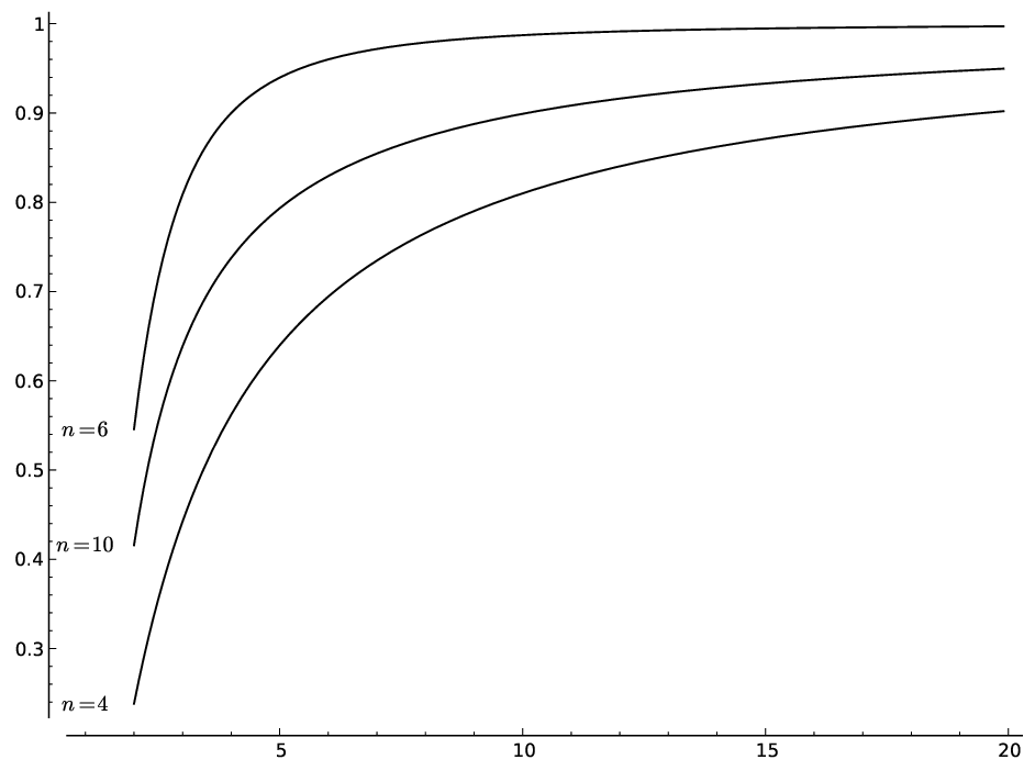
Figure 5: The normalized relative error in Theorem 5.29 (iii)–(iv) for (r,s)=(2,2)(r,s)=(2,2).

Figure 5shows plots of (𝖰r,n,s​(𝐪)−ηr,n,s​(𝐪))/(ηr,n,s​(𝐪)​𝐪−δ)({\mathsf{Q}}_{r,n,s}(\mathbf{q})-\eta_{r,n,s}(\mathbf{q}))/(\eta_{r,n,s}(\mathbf{q})\mathbf{q}^{-\delta}) for r=2r=2, s=2s=2 and n=4,6,10n=4,6,10, as we substitute for 𝐪\mathbf{q} real numbers from 22 to 2020.

5.88.

As noted in 4.32 for reducible polynomials, the relative error term is (essentially) exponentially decreasing in the input size, and exponentially decaying in any of the parameters rr, nn, ss, and log2⁡q\log_{2}q, when the other three are fixed.

In the bivariate case, von zur Gathen (2008, Theorem 3.1) approximates the quotient #​Q2,n,s​(𝔽q)/#​P2,n​(𝔽q)\#Q_{2,n,s}(\mathbb{F}_{q})/\#P_{2,n}(\mathbb{F}_{q}) (using our notation) by

q−(2ns−s2+3s−4)/2(1+q−1)​(1−q−n+s−1)1−q−n−1,q^{-(2ns-s^{2}+3s-4)/2}\frac{(1+q^{-1})(1-q^{-n+s-1})}{1-q^{-n-1}},

which equals the term η2,n,s​(q)/#​P2,n​(𝔽q)\eta_{2,n,s}(q)/\#P_{2,n}(\mathbb{F}_{q}) derived from our analysis above.

We append handy bounds using 4.33.

5.89.

For r,s,q≥2r,s,q\geq 2, and n≥sn\geq s, we have

12​q(r+n−sr)+r−1≤#​Qr,n,s​(𝔽q)≤10​q(r+n−sr)+r−1,\displaystyle\frac{1}{2}q^{\binom{r+n-s}{r}+r-1}\leq\#Q_{r,n,s}(\mathbb{F}_{q})\leq 10q^{\binom{r+n-s}{r}+r-1}, (5.90)
12​q−(r+nr)+(r+n−sr)+r≤#​Qr,n,s​(𝔽q)#​Pr,n​(𝔽q)≤5​q−(r+nr)+(r+n−sr)+r,\displaystyle\frac{1}{2}q^{-\binom{r+n}{r}+\binom{r+n-s}{r}+r}\leq\frac{\#Q_{r,n,s}(\mathbb{F}_{q})}{\#P_{r,n}(\mathbb{F}_{q})}\leq 5q^{-\binom{r+n}{r}+\binom{r+n-s}{r}+r}, (5.91)
16​q−(r+n−1r)+(r+n−sr)≤#​Qr,n,s​(𝔽q)#​Rr,n​(𝔽q)≤19​q−(r+n−1r)+(r+n−sr).\displaystyle\frac{1}{6}q^{-\binom{r+n-1}{r}+\binom{r+n-s}{r}}\leq\frac{\#Q_{r,n,s}(\mathbb{F}_{q})}{\#R_{r,n}(\mathbb{F}_{q})}\leq 19q^{-\binom{r+n-1}{r}+\binom{r+n-s}{r}}. (5.92)

We conclude this section with bounds for the number of ss-powerfree polynomials.

5.93.

Let r,s,q≥2r,s,q\geq 2, n≥0n\geq 0, and ηr,n,s\eta_{r,n,s} and δ\delta as in Theorem 5.29. We have

#​Pr,n​(𝔽q)−3​ηr,n,s​(q)≤#​Sr,n,s​(𝔽q)≤#​Pr,n​(𝔽q),\#P_{r,n}(\mathbb{F}_{q})-3\eta_{r,n,s}(q)\leq\#S_{r,n,s}(\mathbb{F}_{q})\leq\#P_{r,n}(\mathbb{F}_{q}), (5.94)

and more precisely

#​Sr,n,s​(𝔽q)={#​Pr,n​(𝔽q)for n<s,#​Pr,n​(𝔽q)−ηr,n,s​(q)for s≤n<2​s,#​Pr,n​(𝔽q)−ηr,n,s​(q)​(1+q−δ⋅1−q−(n+r−2​s−1r−1)1−q−(n+r−s−1r−1)CLOSE⋅(1−q−r(r+1)/21−q−r−q−r(r−1)/21−q−r1−q−1))for 2​s≤n<3​s,\#S_{r,n,s}(\mathbb{F}_{q})=\begin{cases}\#P_{r,n}(\mathbb{F}_{q})&\text{for $n<s$,}\\ \#P_{r,n}(\mathbb{F}_{q})-\eta_{r,n,s}(q)&\text{for $s\leq n<2s$,}\\ \#P_{r,n}(\mathbb{F}_{q})-\eta_{r,n,s}(q)\bigg(1+q^{-\delta}\cdot\frac{1-q^{-\binom{n+r-2s-1}{r-1}}}{1-q^{-\binom{n+r-s-1}{r-1}}}&\\ \quad\cdot\Big(\frac{1-q^{-r(r+1)/2}}{1-q^{-r}}-q^{-r(r-1)/2}\frac{1-q^{-r}}{1-q^{-1}}\Big)\bigg)&\text{for $2s\leq n<3s$,}\end{cases} (5.95)
|#​Sr,6,2​(𝔽q)−(#​Pr,n​(𝔽q)−ηr,6,2​(q))|≤ηr,6,2​(q)⋅2​q−δ+(r−2)​(r−1)​(r+3)/6,\left|\#S_{r,6,2}(\mathbb{F}_{q})-(\#P_{r,n}(\mathbb{F}_{q})-\eta_{r,6,2}(q))\right|\leq\eta_{r,6,2}(q)\cdot 2q^{-\delta+(r-2)(r-1)(r+3)/6}, (5.96)

and for n≥3​sn\geq 3s with (n,s)≠(6,2)(n,s)\neq(6,2)

|#​Sr,n,s​(𝔽q)−(#​Pr,n​(𝔽q)−ηr,n,s​(q))|≤ηr,n,s​(q)⋅6​q−δ.\left|\#S_{r,n,s}(\mathbb{F}_{q})-(\#P_{r,n}(\mathbb{F}_{q})-\eta_{r,n,s}(q))\right|\leq\eta_{r,n,s}(q)\cdot 6q^{-\delta}. (5.97)

6 Relatively irreducible polynomials

A polynomial over FF is absolutely irreducible if it is irreducible over an algebraic closure of FF, and relatively irreducible if it is irreducible over FF but factors over some extension field of FF. We define

Ar,n​(F)\displaystyle A_{r,n}(F) ={f∈Pr,n​(F):f​ is absolutely irreducible}⊆Ir,n​(F),\displaystyle=\{f\in P_{r,n}(F)\colon f\text{ is absolutely irreducible}\}\subseteq I_{r,n}(F), (6.1)
Er,n​(F)\displaystyle E_{r,n}(F) =Ir,n​(F)∖Ar,n​(F).\displaystyle=I_{r,n}(F)\setminus A_{r,n}(F). (6.2)

As before, we restrict ourselves to finite fields and recall that all our polynomials are monic. For a field extension 𝔽qk\mathbb{F}_{q^{k}} over 𝔽q\mathbb{F}_{q} of degree kk, we consider the Galois group Gk=Gal⁡(𝔽qk:𝔽q)≅ℤkG_{k}=\Gal(\mathbb{F}_{q^{k}}:\mathbb{F}_{q})\cong\mathbb{Z}_{k}. It acts on 𝔽qk​[x]\mathbb{F}_{q^{k}}[x] coefficientwise and we have the “norm” map

φr,n,k:Pr,n/k​(𝔽qk)\displaystyle\varphi_{r,n,k}\colon P_{r,n/k}(\mathbb{F}_{q^{k}}) →Pr,n​(𝔽q),\displaystyle\to P_{r,n}(\mathbb{F}_{q}),
g\displaystyle g ↦∏σ∈Gkgσ,\displaystyle\mapsto\prod_{\sigma\in G_{k}}g^{\sigma},

for each kk dividing nn. Since (φr,n,k​(g))τ=φr,n,k​(g)(\varphi_{r,n,k}(g))^{\tau}=\varphi_{r,n,k}(g) for any τ∈Gk\tau\in G_{k} and therefore φr,n,k​(g)∈Pr,n​(𝔽q)\varphi_{r,n,k}(g)\in P_{r,n}(\mathbb{F}_{q}), this map is well-defined.

Relatively irreducible polynomials in Pr,n​(𝔽q)P_{r,n}(\mathbb{F}_{q}) are the product of all conjugates of an irreducible polynomial gg defined over some extension field 𝔽qk\mathbb{F}_{q^{k}}. If gg itself is relatively irreducible over 𝔽qk\mathbb{F}_{q^{k}}, then there exists an appropriate multiple jj of kk and h∈Pr,n/j​(𝔽qj)h\in P_{r,n/j}(\mathbb{F}_{q^{j}}) with the same image φr,n,k​(g)=φr,n,j​(h)\varphi_{r,n,k}(g)=\varphi_{r,n,j}(h) in Pr,n​(𝔽q)P_{r,n}(\mathbb{F}_{q}) and the property that hh is absolutely irreducible. So, every relatively irreducible polynomial is contained in φr,n,k​(Ar,n/k​(𝔽qk))\varphi_{r,n,k}(A_{r,n/k}(\mathbb{F}_{q^{k}})) for a unique k>1k>1 dividing nn. Furthermore, the absolutely irreducible polynomials in Pr,n​(𝔽q)P_{r,n}(\mathbb{F}_{q}) are exactly those in φr,n,1​(Ar,n​(𝔽q))\varphi_{r,n,1}(A_{r,n}(\mathbb{F}_{q})), and we summarize

Ar,n​(𝔽q)\displaystyle A_{r,n}(\mathbb{F}_{q}) =φr,n,1​(Ar,n​(𝔽q)),\displaystyle=\varphi_{r,n,1}(A_{r,n}(\mathbb{F}_{q})), (6.3)
Er,n​(𝔽q)\displaystyle E_{r,n}(\mathbb{F}_{q}) ⊆⋃1<k|nφr,n,k​(Ar,n/k​(𝔽qk)).\displaystyle\subseteq\bigcup_{1<k\,\mid\,n}\varphi_{r,n,k}(A_{r,n/k}(\mathbb{F}_{q^{k}})). (6.4)

In order to replace the latter by an equality, we let

Ar,n/k+​(𝔽qk)=Ar,n/k​(𝔽qk)∖⋃s|k,s≠kAr,n/k​(𝔽qs)A_{r,n/k}^{+}(\mathbb{F}_{q^{k}})=A_{r,n/k}(\mathbb{F}_{q^{k}})\setminus\bigcup_{s\,\mid\,k,\,s\neq k}A_{r,n/k}(\mathbb{F}_{q^{s}}) (6.5)

be the set of absolutely irreducible polynomials over 𝔽qk\mathbb{F}_{q^{k}} that are not defined over a proper subfield containing 𝔽q\mathbb{F}_{q}, and

Ir,n,k​(𝔽q)=φr,n,k​(Ar,n/k+​(𝔽qk)).I_{r,n,k}(\mathbb{F}_{q})=\varphi_{r,n,k}(A_{r,n/k}^{+}(\mathbb{F}_{q^{k}})). (6.6)
6.7.
  1. (i)

    We have the disjoint union

    Ir,n​(𝔽q)=⋃k|n˙​Ir,n,k​(𝔽q)I_{r,n}(\mathbb{F}_{q})=\dot{\bigcup_{k\,\mid\,n}}I_{r,n,k}(\mathbb{F}_{q}) (6.8)

    and more precisely

    Ar,n​(𝔽q)\displaystyle A_{r,n}(\mathbb{F}_{q}) =Ir,n,1​(𝔽q),\displaystyle=I_{r,n,1}(\mathbb{F}_{q}), (6.9)
    Er,n​(𝔽q)\displaystyle E_{r,n}(\mathbb{F}_{q}) =⋃1<k|n˙​Ir,n,k​(𝔽q).\displaystyle=\dot{\bigcup_{1<k\,\mid\,n}}I_{r,n,k}(\mathbb{F}_{q}). (6.10)
  2. (ii)

    #​Ir,n,k​(𝔽q)=1k​#​Ar,n/k+​(𝔽qk)\#I_{r,n,k}(\mathbb{F}_{q})=\frac{1}{k}\#A_{r,n/k}^{+}(\mathbb{F}_{q^{k}}).

Proof.
  1. (i)

    Let g∈Ar,n/k​(𝔽qk)g\in A_{r,n/k}(\mathbb{F}_{q^{k}}). By definition, gg is monic. The kk conjugates gσg^{\sigma}, for σ∈Gk\sigma\in G_{k}, are pairwise non-associate if and only if the coefficients are not contained in some proper subfield of 𝔽qk\mathbb{F}_{q^{k}}. This shows

    Ir,n,k​(𝔽q)⊆Ir,n​(𝔽q).I_{r,n,k}(\mathbb{F}_{q})\subseteq I_{r,n}(\mathbb{F}_{q}). (6.11)

    Let f∈Ir,n​(𝔽q)f\in I_{r,n}(\mathbb{F}_{q}). Then f=φr,n,k​(g)f=\varphi_{r,n,k}(g) for some g∈Ar,n/k​(𝔽qk)g\in A_{r,n/k}(\mathbb{F}_{q^{k}}), with kk dividing nn as observed in (6.4). If gg has coefficients from a subfield of 𝔽qk\mathbb{F}_{q^{k}}, say g∈Ar,n/k​(𝔽qs)g\in A_{r,n/k}(\mathbb{F}_{q^{s}}) for some s<ks<k dividing kk, then gσg^{\sigma} equals gg for some σ∈Gk∖{id}\sigma\in G_{k}\setminus\{\id\}. Taking the smallest such ss and

    h=∏τ∈Gsgτ∈Ir,n,k/s​(𝔽q),h=\prod_{\tau\in G_{s}}g^{\tau}\in I_{r,n,k/s}(\mathbb{F}_{q}),

    we have hk/s=φr,n,k​(g)h^{k/s}=\varphi_{r,n,k}(g). Hence φr,n,k​(g)\varphi_{r,n,k}(g) is a (k/s)(k/s)-th power and therefore reducible, in contradiction to the choice of ff. This shows that g∈Ar,n/k+​(𝔽qk)g\in A_{r,n/k}^{+}(\mathbb{F}_{q^{k}}) and a fortiori

    Ir,n​(𝔽q)⊆⋃k|nIr,n,k​(𝔽q).I_{r,n}(\mathbb{F}_{q})\subseteq\bigcup_{k\,\mid\,n}I_{r,n,k}(\mathbb{F}_{q}). (6.12)

    The disjointness follows from the fact that the factorization of φr,n,k​(g)\varphi_{r,n,k}(g) for any g∈Ar,n/k+​(𝔽qk)g\in A_{r,n/k}^{+}(\mathbb{F}_{q^{k}}) has exactly kk irreducible factors over 𝔽qn\mathbb{F}_{q^{n}}, and (6.8) follows with (6.11).

    Finally, (6.9) and (6.10) follow from (6.3) and (6.2), respectively.

  2. (ii)

    Let g,h∈Ir,n/k​(𝔽qk)g,h\in I_{r,n/k}(\mathbb{F}_{q^{k}}). Then φr,n,k​(g)=φr,n,k​(h)\varphi_{r,n,k}(g)=\varphi_{r,n,k}(h) if and only if h=gσh=g^{\sigma} for some automorphism σ∈Gk\sigma\in G_{k}. Sufficiency is a direct computation and necessity follows from the unique factorization of φr,n,k​(g)\varphi_{r,n,k}(g) and φr,n,k​(h)\varphi_{r,n,k}(h) over 𝔽qk\mathbb{F}_{q^{k}}. Therefore, the size of each fibre of φr,n,k\varphi_{r,n,k} on Ar,n/k+​(𝔽qk)A_{r,n/k}^{+}(\mathbb{F}_{q^{k}}) is #​Gk=k\#G_{k}=k. ∎

We omit the parameter rr from the notation of the generating functions and their coefficients. The generating function A+​(𝔽qk){\mathrm{A}}^{+}(\mathbb{F}_{q^{k}}) of #​Ar,n+​(𝔽qk)\#A_{r,n}^{+}(\mathbb{F}_{q^{k}}) is related to the generating function A⁡(𝔽q){\mathrm{A}}(\mathbb{F}_{q}) of #​Ar,n​(𝔽q)\#A_{r,n}(\mathbb{F}_{q}) by definition (6.5) and we find by inclusion-exclusion

A+​(𝔽qk)=∑s|kμ⁡(k/s)​A​(𝔽qs).{\mathrm{A}}^{+}(\mathbb{F}_{q^{k}})=\sum_{s\,\mid\,k}\mu(k/s){\mathrm{A}}(\mathbb{F}_{q^{s}}). (6.13)

With (6.8) and 6.7 (ii), we relate this to the generating function I⁡(𝔽q){\mathrm{I}}(\mathbb{F}_{q}) of irreducible polynomials as introduced in Section 3 and obtain

[zn]​I​(𝔽q)\displaystyle[z^{n}]{\mathrm{I}}(\mathbb{F}_{q}) =∑k|n1k​∑s|kμ⁡(k/s)⋅[zn/k]​A​(𝔽qs),\displaystyle=\sum_{k\,\mid\,n}\frac{1}{k}\sum_{s\,\mid\,k}\mu(k/s)\cdot[z^{n/k}]{\mathrm{A}}(\mathbb{F}_{q^{s}}), (6.14)
[zn]​A​(𝔽q)\displaystyle[z^{n}]{\mathrm{A}}(\mathbb{F}_{q}) =∑k|n1k​∑s|kμ⁡(s)⋅[zn/k]​I​(𝔽qs)\displaystyle=\sum_{k\,\mid\,n}\frac{1}{k}\sum_{s\,\mid\,k}\mu(s)\cdot[z^{n/k}]{\mathrm{I}}(\mathbb{F}_{q^{s}}) (6.15)

with Möbius inversion.

A Maple program to compute the latter is shown in Figure 6.

absirreds:=proc(n,r) local k,s: option remember: add(1/k*add(mobius(s)*subs(q=qˆs,coeff(irreduciblesGF( z,n/k,r),zˆ(n/k))),s=divisors(k)),k=divisors(n))end:absirredsGF:=proc(z,N,r) local k,s: option remember: sum(’absirreds(k,r)*zˆk’,k=1..N)end:relirredsGF:=proc(z,N,r) option remember: irreduciblesGF(z,N,r)-absirredsGF(z,N,r);end:relirreds:=proc(n,r) coeff(sort(expand(relirredsGF(z,n,r))),zˆn):end:

Figure 6: Maple program to compute the number of relatively irreducible polynomials in rr variables of degree nn.

Exact values for #​E2,n​(𝔽q)\#E_{2,n}(\mathbb{F}_{q}) with n≤6n\leq 6 are given in von zur Gathen (2008, Table 4.1). We extend this in Table 4.

Table 4: Exact values of #​Er,n​(𝔽q)\#E_{r,n}(\mathbb{F}_{q}) for small values of rr and nn.

For an explicit formula, we combine the expression for In​(𝔽q)=In{\mathrm{I}}_{n}(\mathbb{F}_{q})={\mathrm{I}}_{n} from Theorem 3.11 with (6.15).

6.16.

For r,n≥1r,n\geq 1, q≥2q\geq 2, MnM_{n} as in (3.10), and Pn​(𝔽q)=Pn{\mathrm{P}}_{n}(\mathbb{F}_{q})={\mathrm{P}}_{n} as in (3.4), we have

A0​(𝔽q)\displaystyle{\mathrm{A}}_{0}(\mathbb{F}_{q}) =0,\displaystyle=0, (6.17)
An​(𝔽q)\displaystyle{\mathrm{A}}_{n}(\mathbb{F}_{q}) =−∑s​∣k∣​nμ⁡(s)k∑m|n/kμ⁡(m)m∑j∈Mn/(k​m)(−1)|j||j|Pj1(𝔽qs)Pj2(𝔽qs)⋯Pj|j|(𝔽qs),\displaystyle=-\sum_{s\,\mid\,k\,\mid\,n}\frac{\mu(s)}{k}\sum_{m\,\mid\,n/k}\frac{\mu(m)}{m}\sum_{j\in M_{n/(km)}}\frac{(-1)^{\lvert j\rvert}}{\lvert j\rvert}{\mathrm{P}}_{j_{1}}(\mathbb{F}_{q^{s}}){\mathrm{P}}_{j_{2}}(\mathbb{F}_{q^{s}})\cdots{\mathrm{P}}_{j_{\lvert j\rvert}}(\mathbb{F}_{q^{s}}), (6.18)
E0​(𝔽q)\displaystyle{\mathrm{E}}_{0}(\mathbb{F}_{q}) =0,\displaystyle=0, (6.19)
En​(𝔽q)\displaystyle{\mathrm{E}}_{n}(\mathbb{F}_{q}) =−∑1<k|n1k∑s|kμ(s)In/k(𝔽qs)\displaystyle=-\sum_{1<k\,\mid\,n}\frac{1}{k}\sum_{s\,\mid\,k}\mu(s){\mathrm{I}}_{n/k}(\mathbb{F}_{q^{s}}) (6.20)
=∑1<k|n1k∑s|km|n/kμ⁡(s)​μ​(m)m∑j∈Mn/(k​m)(−1)|j||j|Pj1(𝔽qs)Pj2(𝔽qs)⋯Pj|j|(𝔽qs).\displaystyle=\sum_{1<k\,\mid\,n}\frac{1}{k}\sum_{\begin{subarray}{c}s\,\mid\,k\\ m\,\mid\,n/k\end{subarray}}\frac{\mu(s)\mu(m)}{m}\sum_{j\in M_{n/(km)}}\frac{(-1)^{\lvert j\rvert}}{\lvert j\rvert}{\mathrm{P}}_{j_{1}}(\mathbb{F}_{q^{s}}){\mathrm{P}}_{j_{2}}(\mathbb{F}_{q^{s}})\cdots{\mathrm{P}}_{j_{\lvert j\rvert}}(\mathbb{F}_{q^{s}}). (6.21)

We check that for r=1r=1 we obtain the expected result

An​(𝔽q)={qif n=1,0if n>1.{\mathrm{A}}_{n}(\mathbb{F}_{q})=\begin{cases}q&\text{if $n=1$},\\ 0&\text{if $n>1$}.\end{cases} (6.22)

To this end, we use the well-known fact that

∑s|nμ⁡(s)={1if n=1,0if n>1.\sum_{s\,\mid\,n}\mu(s)=\begin{cases}1&\text{if $n=1$},\\ 0&\text{if $n>1$}.\end{cases} (6.23)

From (6.29) and (3.21) we have

n​An​(𝔽q)\displaystyle n{\mathrm{A}}_{n}(\mathbb{F}_{q}) =∑s​∣k∣​nt|n/kμ⁡(s)​μ​(t)​qn​sk​t=∑s​∣k∣​na|n/kμ⁡(s)​μ​(n/(k​a))​qs​a\displaystyle=\sum_{\begin{subarray}{c}s\,\mid\,k\,\mid\,n\\ t\,\mid\,n/k\end{subarray}}\mu(s)\mu(t)q^{\frac{ns}{kt}}=\sum_{\begin{subarray}{c}s\,\mid\,k\,\mid\,n\\ a\,\mid\,n/k\end{subarray}}\mu(s)\mu(n/(ka))q^{sa} (6.24)
=∑m|nqm​∑s​∣k∣​nm=s​a,a|n/kμ⁡(s)​μ​(n/(k​a))=∑m|nqm​∑s|mμ⁡(s)​∑s​∣k∣​nm/s|n/kμ⁡(n​s/(m​k))\displaystyle=\sum_{m\,\mid\,n}q^{m}\sum_{\begin{subarray}{c}s\,\mid\,k\,\mid\,n\\ m=sa,\,a\,\mid\,n/k\end{subarray}}\mu(s)\mu(n/(ka))=\sum_{m\,\mid\,n}q^{m}\sum_{s\,\mid\,m}\mu(s)\sum_{\begin{subarray}{c}s\,\mid\,k\,\mid\,n\\ m/s\,\mid\,n/k\end{subarray}}\mu(ns/(mk)) (6.25)
=∑m|nqm​∑s|mμ⁡(s)​∑j|n/mμ⁡(n/(m​j))\displaystyle=\sum_{m\,\mid\,n}q^{m}\sum_{s\,\mid\,m}\mu(s)\sum_{j\,\mid\,n/m}\mu(n/(mj)) (6.26)
=∑m|nqm​∑s|mμ⁡(s)​∑i|n/mμ⁡(i)={qif n=1,0if n>1,\displaystyle=\sum_{m\,\mid\,n}q^{m}\sum_{s\,\mid\,m}\mu(s)\sum_{i\,\mid\,n/m}\mu(i)=\begin{cases}q&\text{if $n=1$},\\ 0&\text{if $n>1$},\end{cases} (6.27)

where a=n/(k​t)a=n/(kt), m=a​sm=as, j=k/sj=k/s, and i=n/(m​j)i=n/(mj).

The remainder of this section deals with the case r≥2r\geq 2. For the approach by symbolic generating functions, we define, with 𝖨⁡(𝐪,z){\mathsf{I}}(\mathbf{q},z) as in (3.25), the two power series 𝖠,𝖤∈ℚ⁡(𝐪)​⟦z⟧{\mathsf{A}},{\mathsf{E}}\in\mathbb{Q}(\mathbf{q})\left\llbracket z\right\rrbracket by

𝖠0​(𝐪)\displaystyle{\mathsf{A}}_{0}(\mathbf{q}) =𝖨0​(𝐪)=0,\displaystyle={\mathsf{I}}_{0}(\mathbf{q})=0, (6.28)
𝖠n​(𝐪)\displaystyle{\mathsf{A}}_{n}(\mathbf{q}) =∑k|n1k​∑s|kμ⁡(s)​𝖨n/k​(𝐪s)∈ℤ⁡[𝐪]​ for ​n>0,\displaystyle=\sum_{k\,\mid\,n}\frac{1}{k}\sum_{s\,\mid\,k}\mu(s){\mathsf{I}}_{n/k}(\mathbf{q}^{s})\in\mathbb{Z}[\mathbf{q}]\text{ for }n>0, (6.29)
𝖠⁡(𝐪,z)\displaystyle{\mathsf{A}}(\mathbf{q},z) =∑n≥0𝖠n​(𝐪)​zn∈ℤ⁡[𝐪]​⟦z⟧,\displaystyle=\sum_{n\geq 0}{\mathsf{A}}_{n}(\mathbf{q})z^{n}\in\mathbb{Z}[\mathbf{q}]\left\llbracket z\right\rrbracket, (6.30)
𝖤⁡(𝐪,z)\displaystyle{\mathsf{E}}(\mathbf{q},z) =𝖨⁡(𝐪,z)−𝖠⁡(𝐪,z)\displaystyle={\mathsf{I}}(\mathbf{q},z)-{\mathsf{A}}(\mathbf{q},z) (6.31)
=−∑1<k|n1k∑s|kμ(s)𝖨n/k(𝐪s)∈ℤ[𝐪]⟦z⟧.\displaystyle=-\sum_{1<k\,\mid\,n}\frac{1}{k}\sum_{s\,\mid\,k}\mu(s){\mathsf{I}}_{n/k}(\mathbf{q}^{s})\in\mathbb{Z}[\mathbf{q}]\left\llbracket z\right\rrbracket. (6.32)

Then

𝖠n​(q)=#​Ar,n​(𝔽q),𝖤n​(q)=#​Er,n​(𝔽q).\begin{split}{\mathsf{A}}_{n}(q)&=\#A_{r,n}(\mathbb{F}_{q}),\\ {\mathsf{E}}_{n}(q)&=\#E_{r,n}(\mathbb{F}_{q}).\end{split} (6.33)

The inner sum of (6.32) has degree deg𝐪⁡𝖨n/k​(𝐪k)\deg_{\mathbf{q}}{\mathsf{I}}_{n/k}(\mathbf{q}^{k}) in 𝐪\mathbf{q}. Let nn be composite and ℓ\ell its smallest prime divisor. For k=ℓk=\ell, this inner sum consists of only two terms and we find

𝖤n​(𝐪)\displaystyle{\mathsf{E}}_{n}(\mathbf{q}) =1ℓ​(𝖨n/ℓ​(𝐪ℓ)−𝖨n/ℓ​(𝐪))−∑ℓ<k|n1k​∑s|kμ⁡(s)​𝖨n/k​(𝐪s)\displaystyle=\frac{1}{\ell}({\mathsf{I}}_{n/\ell}(\mathbf{q}^{\ell})-{\mathsf{I}}_{n/\ell}(\mathbf{q}))-\sum_{\ell<k\,\mid\,n}\frac{1}{k}\sum_{s|k}\mu(s){\mathsf{I}}_{n/k}(\mathbf{q}^{s}) (6.34)
=1ℓ​(𝖯n/ℓ​(𝐪ℓ)−𝖱n/ℓ​(𝐪ℓ)−𝖨n/ℓ​(𝐪))+O⁡(𝐪maxℓ<k|n⁡wr,n​(k)),\displaystyle=\frac{1}{\ell}({\mathsf{P}}_{n/\ell}(\mathbf{q}^{\ell})-{\mathsf{R}}_{n/\ell}(\mathbf{q}^{\ell})-{\mathsf{I}}_{n/\ell}(\mathbf{q}))+O(\mathbf{q}^{\max_{\ell<k\mid n}w_{r,n}(k)}), (6.35)

with

wr,n​(k)=deg𝐪⁡(𝖨n/k​(𝐪k))=deg𝐪⁡(𝖯n/k​(𝐪k))=k⁡((r+n/k)r¯/r!−1)w_{r,n}(k)=\deg_{\mathbf{q}}({\mathsf{I}_{n/k}(\mathbf{q}^{k})})=\deg_{\mathbf{q}}({\mathsf{P}}_{n/k}(\mathbf{q}^{k}))=k((r+n/k)^{\underline{r}}/r!-1) (6.36)

for any divisor kk of nn. Table 5 lists the degree in 𝐪\mathbf{q} for all summands in (6.35). We consider wr,nw_{r,n} as a function on the real interval [1,n][1,n], see Figure 7.

summand deg𝐪\deg_{\mathbf{q}}
𝖯n/ℓ​(𝐪ℓ){\mathsf{P}}_{n/\ell}(\mathbf{q}^{\ell}) ℓ⁡(br,n/ℓ−1)=wr,n​(ℓ)\ell(b_{r,n/\ell}-1)=w_{r,n}(\ell)
𝖱n/ℓ​(𝐪ℓ){\mathsf{R}}_{n/\ell}(\mathbf{q}^{\ell}) ℓ⁡(br,n/ℓ−1+r−1)=wr,n​(ℓ)−ℓ⁡(br−1,n/ℓ−r)\ell(b_{r,n/\ell-1}+r-1)=w_{r,n}(\ell)-\ell(b_{r-1,n/\ell}-r)
𝖨n/ℓ​(𝐪){\mathsf{I}}_{n/\ell}(\mathbf{q}) br,n/ℓ−1=1ℓ​wr,n​(ℓ)b_{r,n/\ell}-1=\frac{1}{\ell}w_{r,n}(\ell)
∑ℓ<k|n𝖨n/k​(𝐪k)\sum_{\ell<k\,\mid\,n}{\mathsf{I}}_{n/k}(\mathbf{q}^{k}) ≤maxℓ<k|n⁡wr,n​(k)\leq\max_{\ell<k\,\mid\,n}w_{r,n}(k)
Table 5: Summands of 𝖤{\mathsf{E}} and their degrees in 𝐪\mathbf{q}.
Refer to caption
Figure 7: Graphs for w2,n​(k)w_{2,n}(k) on [ℓ,n][\ell,n] for composite nn in the range from 44 to 1010, where ℓ\ell denotes the smallest prime divisor of nn. The dots represent the values at divisors of nn.
6.37.

Let r≥2r\geq 2, nn be composite, ℓ\ell the smallest and k2k_{2} the second smallest divisor of nn greater than 11.

  1. (i)

    The function wr,n​(k)w_{r,n}(k) is strictly decreasing in kk on [1,n][1,n].

  2. (ii)

    For composite n≠4,6n\neq 4,6, we have

    wr,n​(ℓ)−wr,n​(k2)−wr−1,n​(ℓ)≥0.w_{r,n}(\ell)-w_{r,n}(k_{2})-w_{r-1,n}(\ell)\geq 0. (6.38)
  3. (iii)

    For composite n>ℓ​k2n>\ell k_{2} different from 1212, we have

    wr,n​(ℓ)−wr,n​(k2)−wr−1,n​(ℓ)≥log2⁡n−2.w_{r,n}(\ell)-w_{r,n}(k_{2})-w_{r-1,n}(\ell)\geq\log_{2}n-2. (6.39)

    This also holds if n=12n=12 and r≥3r\geq 3.

The inequality (6.38) is false when nn is 44 or 66, and (6.39) is false for n=12n=12, r=2r=2.

Proof.

(i) We compute

wr,n′​(k)\displaystyle w_{r,n}^{\prime}(k) =(r+n/k)r¯r!−nr!​k​∑1≤i≤r(r+n/k)r¯i+n/k−1\displaystyle=\frac{(r+n/k)^{\underline{r}}}{r!}-\frac{n}{r!k}\sum_{1\leq i\leq r}\frac{(r+n/k)^{\underline{r}}}{i+n/k}-1 (6.40)
=(r+n/k)r¯r!​(1−∑1≤i≤r11+i​kn)−1.\displaystyle=\frac{(r+n/k)^{\underline{r}}}{r!}\Bigl(1-\sum_{1\leq i\leq r}\frac{1}{1+i\frac{k}{n}}\Bigr)-1. (6.41)

If r≥3r\geq 3, then

∑1≤i≤r11+i​kn≥∑1≤i≤311+i>1\sum_{1\leq i\leq r}\frac{1}{1+i\frac{k}{n}}\geq\sum_{1\leq i\leq 3}\frac{1}{1+i}>1

for all 1≤k≤n1\leq k\leq n, which proves wr,n′​(k)<0w_{r,n}^{\prime}(k)<0.

If r=2r=2, we evaluate (6.41) as

w2,n′​(k)=(1+n/k)​(2+n/k)2​(1−11+k/n−11+2​k/n)−1=−n22​k2w_{2,n}^{\prime}(k)=\frac{(1+n/k)(2+n/k)}{2}\Bigl(1-\frac{1}{1+k/n}-\frac{1}{1+2k/n}\Bigr)-1=-\frac{n^{2}}{2k^{2}} (6.42)

to find w2,n′​(k)<0w_{2,n}^{\prime}(k)<0 for all kk.

For (ii) and (iii), we first show that the sequence ar,n=wr,n​(ℓ)−wr−1,n​(ℓ)−wr,n​(k2)=ℓ​br,n/l−1−k2​(br,n/k2−1)a_{r,n}=w_{r,n}(\ell)-w_{r-1,n}(\ell)-w_{r,n}(k_{2})=\ell b_{r,n/l-1}-k_{2}(b_{r,n/k_{2}}-1) is monotonically increasing in rr. We have

ar,n−ar−1,n=ℓ​br,n/ℓ−2−k2​br,n/k2−1≥0a_{r,n}-a_{r-1,n}=\ell b_{r,n/\ell-2}-k_{2}b_{r,n/k_{2}-1}\geq 0 (6.43)

if and only if

Ar,n=ℓ​(r+n/ℓ−2)r¯k2​(r+n/k2−1)r¯≥1A_{r,n}=\frac{\ell(r+n/\ell-2)^{\underline{r}}}{k_{2}(r+n/k_{2}-1)^{\underline{r}}}\geq 1 (6.44)

and prove the latter by induction on r≥2r\geq 2.

For r=2r=2, we have to prove

n⁡(k2−ℓ)≥2​ℓ​k2.n(k_{2}-\ell)\geq 2\ell k_{2}. (6.45)

If k2=ℓ+1k_{2}=\ell+1, then ℓ=2\ell=2, k2=3k_{2}=3 and since we exclude n=6n=6, we have n≥12n\geq 12 to show (6.45). If k2≥ℓ+2k_{2}\geq\ell+2, we distinguish two cases. Now, k2=nk_{2}=n if and only if n=ℓ2n=\ell^{2}. Since we exclude n=4n=4, we then have ℓ≥3\ell\geq 3 and (6.45) follows. If k2≠nk_{2}\neq n, then k2≤n<nk_{2}\leq\sqrt{n}<n and therefore 2​ℓ​k2<2​n​n≤(k2−ℓ)​n2\ell k_{2}<2\sqrt{n}\sqrt{n}\leq(k_{2}-\ell)n.

For the induction step, we have

Ar,n=Ar−1,n​n/ℓ−2+rn/k2−1+r≥n/ℓ−2+rn/k2−1+r≥1,A_{r,n}=A_{r-1,n}\frac{n/\ell-2+r}{n/k_{2}-1+r}\geq\frac{n/\ell-2+r}{n/k_{2}-1+r}\geq 1,

where the last inequality is equivalent to n⁡(k2−ℓ)≥ℓ​k2n(k_{2}-\ell)\geq\ell k_{2}, which follows from (6.45).

With this monotonicity of ar,na_{r,n} in rr, it is sufficient to check (ii) and (iii) for the smallest admissible value of rr.

  1. (ii)

    We have

    a2,n=n2​(nℓ−nk2−2).a_{2,n}=\frac{n}{2}\Bigl(\frac{n}{\ell}-\frac{n}{k_{2}}-2\Bigr). (6.46)

    For

    • •

      n=ℓ2n=\ell^{2}, ℓ≠4\ell\neq 4,

    • •

      n=ℓ​k2n=\ell k_{2}, n≠6n\neq 6, or

    • •

      n=12n=12,

    this is non-negative by direct computation, and in the remaining case, n>ℓ​k2n>\ell k_{2} different from 1212, by (iii).

  2. (iii)

    For n>ℓ​k2n>\ell k_{2} different from 1212, we have n/ℓ−n/k2≥3n/\ell-n/k_{2}\geq 3 and find with (6.46)

    a2,n≥n2>log2⁡n−2.a_{2,n}\geq\frac{n}{2}>\log_{2}n-2. (6.47)

    For n=12n=12 and r≥3r\geq 3, we compute directly a3,12=10>log2⁡12−2a_{3,12}=10>\log_{2}12-2. ∎

This lemma allows us to order the summands in (6.35) by deg𝐪\deg_{\mathbf{q}}, and the approach by generating functions gives the following result.

6.48.

Let r,n≥2r,n\geq 2, let ℓ\ell be the smallest prime divisor of nn, and

ϵr,n​(𝐪)\displaystyle\epsilon_{r,n}(\mathbf{q}) =𝐪ℓ⁡((r+n/ℓr)−1)ℓ⁡(1−𝐪−ℓ)∈ℚ⁡(𝐪),\displaystyle=\frac{\mathbf{q}^{\ell(\binom{r+n/\ell}{r}-1)}}{\ell(1-\mathbf{q}^{-\ell})}\in\mathbb{Q}(\mathbf{q}), (6.49)
κ\displaystyle\kappa =(ℓ−1)​((r−1+n/ℓr−1)−r)+1.\displaystyle=(\ell-1)(\binom{r-1+n/\ell}{r-1}-r)+1. (6.50)

Then the following hold.

  1. (i)

    𝖤1​(𝐪)=0{\mathsf{E}_{1}}(\mathbf{q})=0.

  2. (ii)

    If nn is prime, then

    𝖤n​(𝐪)\displaystyle{\mathsf{E}_{n}}(\mathbf{q}) =ϵr,n​(𝐪)​(1−𝐪−n​r)​(1−𝐪−r⁡(n−1)​(1−𝐪−r)​(1−𝐪−n)(1−𝐪−1)​(1−𝐪−n​r)).\displaystyle=\epsilon_{r,n}(\mathbf{q})(1-\mathbf{q}^{-nr})\Bigl(1-\mathbf{q}^{-r(n-1)}\frac{(1-\mathbf{q}^{-r})(1-\mathbf{q}^{-n})}{(1-\mathbf{q}^{-1})(1-\mathbf{q}^{-nr})}\Bigr). (6.51)
  3. (iii)

    If nn is composite, then κ≥2\kappa\geq 2 and

    𝖤n​(𝐪)=ϵr,n​(𝐪)​(1+O⁡(𝐪−κ)).{\mathsf{E}_{n}}(\mathbf{q})=\epsilon_{r,n}(\mathbf{q})(1+O(\mathbf{q}^{-\kappa})).
Proof.

For n=1n=1, the sum (6.20) is empty and this shows (i). For n=ℓn=\ell prime, (6.20) simplifies to 𝖤n​(𝐪)=(𝖨1​(𝐪ℓ)−𝖨1​(𝐪))/ℓ=(𝖯1​(𝐪ℓ)−𝖯1​(𝐪))/ℓ{\mathsf{E}}_{n}(\mathbf{q})=({\mathsf{I}}_{1}(\mathbf{q}^{\ell})-{\mathsf{I}}_{1}(\mathbf{q}))/\ell=({\mathsf{P}}_{1}(\mathbf{q}^{\ell})-{\mathsf{P}}_{1}(\mathbf{q}))/\ell, since 𝖨1=𝖯1{\mathsf{I}}_{1}={\mathsf{P}}_{1} by Theorem 3.41 and (ii) follows.

For composite nn, the product (ℓ−1)​(br−1,n/ℓ−r)(\ell-1)(b_{r-1,n/\ell}-r) is positive and therefore κ≥2\kappa\geq 2. We recall the summands of (6.35) in Table 5. 6.37 (i) shows that maxℓ<k|n⁡wr,n​(k)=wr,n​(k2)\max_{\ell<k\,\mid\,n}w_{r,n}(k)=w_{r,n}(k_{2}) and we find

𝖤n​(𝐪)\displaystyle{\mathsf{E}}_{n}(\mathbf{q}) =1ℓ​(𝖯n/ℓ​(𝐪ℓ)−𝖱n/ℓ​(𝐪ℓ)−𝖨n/ℓ​(𝐪))+O⁡(𝐪wr,n​(k2)).\displaystyle=\frac{1}{\ell}({\mathsf{P}}_{n/\ell}(\mathbf{q}^{\ell})-{\mathsf{R}}_{n/\ell}(\mathbf{q}^{\ell})-{\mathsf{I}}_{n/\ell}(\mathbf{q}))+O(\mathbf{q}^{w_{r,n}(k_{2})}). (6.52)

Since br−1,n/ℓ−r>0b_{r-1,n/\ell}-r>0 for composite nn, we identify with 6.37 (i) as main term 𝖯n/ℓ​(𝐪ℓ)/ℓ=ϵr,n​(𝐪)​(1−𝐪−ℓ​br−1,n/ℓ){\mathsf{P}}_{n/\ell}(\mathbf{q}^{\ell})/\ell=\epsilon_{r,n}(\mathbf{q})(1-\mathbf{q}^{-\ell b_{r-1,n/\ell}}). For the summands of

𝖤n​(𝐪)/ϵr,n​(𝐪)=(1−𝐪−ℓ​br−1,n/ℓ)​(1−𝖱n/ℓ​(𝐪ℓ)𝖯n/ℓ​(𝐪ℓ)−𝖨n/ℓ​(𝐪)𝖯n/ℓ​(𝐪ℓ))+O⁡(𝐪wr,n​(k2)−deg𝐪⁡𝖯n/ℓ​(𝐪ℓ)){\mathsf{E}}_{n}(\mathbf{q})/\epsilon_{r,n}(\mathbf{q})=(1-\mathbf{q}^{-\ell b_{r-1,n/\ell}})\Bigl(1-\frac{{\mathsf{R}}_{n/\ell}(\mathbf{q}^{\ell})}{{\mathsf{P}}_{n/\ell}(\mathbf{q}^{\ell})}-\frac{{\mathsf{I}}_{n/\ell}(\mathbf{q})}{{\mathsf{P}}_{n/\ell}(\mathbf{q}^{\ell})}\Bigr)+O(\mathbf{q}^{w_{r,n}(k_{2})-\deg_{\mathbf{q}}{\mathsf{P}}_{n/\ell}(\mathbf{q}^{\ell})}) (6.53)

we find as degrees in 𝐪\mathbf{q}

−ℓ​br−1,n/ℓ\displaystyle-\ell b_{r-1,n/\ell} ≤−κ,\displaystyle\leq-\kappa, (6.54)
deg𝐪⁡𝖱n/ℓ​(𝐪ℓ)−deg𝐪⁡𝖯n/ℓ​(𝐪ℓ)=−ℓ⁡(br−1,n/ℓ−r)\displaystyle\deg_{\mathbf{q}}{\mathsf{R}}_{n/\ell}(\mathbf{q}^{\ell})-\deg_{\mathbf{q}}{\mathsf{P}}_{n/\ell}(\mathbf{q}^{\ell})=-\ell(b_{r-1,n/\ell}-r) ≤−κ,\displaystyle\leq-\kappa, (6.55)
deg𝐪⁡𝖨n/ℓ​(𝐪)−deg𝐪⁡𝖯n/ℓ​(𝐪ℓ)=−(ℓ−1)​(br,n/ℓ−1)\displaystyle\deg_{\mathbf{q}}{\mathsf{I}}_{n/\ell}(\mathbf{q})-\deg_{\mathbf{q}}{\mathsf{P}}_{n/\ell}(\mathbf{q}^{\ell})=-(\ell-1)(b_{r,n/\ell}-1) ≤−κ,\displaystyle\leq-\kappa, (6.56)
wr,n​(k2)−deg𝐪⁡𝖯n/ℓ​(𝐪ℓ)≤−ℓ⁡(br−1,n/ℓ−1)\displaystyle w_{r,n}(k_{2})-\deg_{\mathbf{q}}{\mathsf{P}}_{n/\ell}(\mathbf{q}^{\ell})\leq-\ell(b_{r-1,n/\ell}-1) ≤−κ\displaystyle\leq-\kappa (6.57)

for n≠4,6n\neq 4,6 by 6.37 (ii). When nn is 44 or 66, the last inequality in (6.57) is false, but still

wr,n​(k2)−deg𝐪⁡𝖯n/ℓ​(𝐪ℓ)≤−κ.∎w_{r,n}(k_{2})-\deg_{\mathbf{q}}{\mathsf{P}}_{n/\ell}(\mathbf{q}^{\ell})\leq-\kappa.\mbox{\qed} (6.58)

On closer inspection, it is possible to partition for each composite nn the range for rr into two non-empty intervals, where either the difference in (6.55) or the difference in (6.56) dominates all others. This provides tighter bounds at the cost of further case distinctions.

The combinatorial approach yields the following result.

6.59.

Let r,q≥2r,q\geq 2, and ϵr,n\epsilon_{r,n} and κ\kappa as in Theorem 6.48.

  1. (i)

    #​Er,1​(𝔽q)=0\#E_{r,1}(\mathbb{F}_{q})=0.

  2. (ii)

    If nn is prime, then

    #​Er,n​(𝔽q)=ϵr,n​(q)​(1−q−n​r)​(1−q−r⁡(n−1)​(1−q−r)​(1−q−n)(1−q−1)​(1−q−n​r)),\displaystyle\#E_{r,n}(\mathbb{F}_{q})=\epsilon_{r,n}(q)(1-q^{-nr})\Bigl(1-q^{-r(n-1)}\frac{(1-q^{-r})(1-q^{-n})}{(1-q^{-1})(1-q^{-nr})}\Bigr),\qquad (6.60)
    0≤ϵr,n​(q)−#​Er,n​(𝔽q)≤3​q−r⁡(n−1).\displaystyle 0\leq\epsilon_{r,n}(q)-\#E_{r,n}(\mathbb{F}_{q})\leq 3q^{-r(n-1)}. (6.61)
  3. (iii)

    If nn is composite, then

    |#​Er,n​(𝔽q)−ϵr,n​(q)|≤ϵr,n​(q)⋅3​q−κ.\left|\#E_{r,n}(\mathbb{F}_{q})-\epsilon_{r,n}(q)\right|\leq\epsilon_{r,n}(q)\cdot 3q^{-\kappa}.
Proof.

The exact statements of (i) and (ii) were already shown in Theorem 6.48 and in (6.60) we have q−r⁡(n−1)/16q^{-r(n-1)}/16 as upper bound for q−n​rq^{-nr} and 32​q−r⁡(n−1)/1532q^{-r(n-1)}/15 as upper bound for the last subtracted term.

For (iii), let ℓ\ell be the smallest and k2k_{2} the second smallest divisor of nn greater than 11. We prove that

#​Er,n​(𝔽q)\displaystyle\#E_{r,n}(\mathbb{F}_{q}) ≥ϵr,n​(q)​(1−3​q−κ),\displaystyle\geq\epsilon_{r,n}(q)(1-3q^{-\kappa}), (6.62)
#​Er,n​(𝔽q)\displaystyle\#E_{r,n}(\mathbb{F}_{q}) ≤ϵr,n(q)(1+2q−ℓ⁡(br−1,n/ℓ−1))for n≠4,6,\displaystyle\leq\epsilon_{r,n}(q)(1+2q^{-\ell(b_{r-1,n/\ell}-1)})\quad\text{for $n\neq 4,6$}, (6.63)
#​Er,n​(𝔽q)\displaystyle\#E_{r,n}(\mathbb{F}_{q}) ≤ϵr,n(q)(1+q−κ)for n=4,6.\displaystyle\leq\epsilon_{r,n}(q)(1+q^{-\kappa})\quad\text{for $n=4,6$.} (6.64)

We begin with (6.62) and have from 6.7 (ii)

#​Er,n​(𝔽q)\displaystyle\#E_{r,n}(\mathbb{F}_{q}) ≥#​Ir,n,ℓ​(𝔽q)=1ℓ​#​Ar,n/ℓ+​(𝔽qℓ)\displaystyle\geq\#I_{r,n,\ell}(\mathbb{F}_{q})=\frac{1}{\ell}\#A_{r,n/\ell}^{+}(\mathbb{F}_{q^{\ell}}) (6.65)
=1ℓ​(#​Ir,n/ℓ​(𝔽qℓ)−#​Ir,n/ℓ​(𝔽q)),\displaystyle=\frac{1}{\ell}(\#I_{r,n/\ell}(\mathbb{F}_{q^{\ell}})-\#I_{r,n/\ell}(\mathbb{F}_{q})), (6.66)

since ℓ\ell is prime and there are no proper intermediate fields between 𝔽q\mathbb{F}_{q} and 𝔽qℓ\mathbb{F}_{q^{\ell}}. With the lower bound on the number of irreducible polynomials from 4.36 this yields

#​Er,n​(𝔽q)\displaystyle\#E_{r,n}(\mathbb{F}_{q}) ≥1ℓ​(#​Pr,n/ℓ​(𝔽qℓ)−2​ρr,n/ℓ​(qℓ)−#​Pr,n/ℓ​(𝔽q))\displaystyle\geq\frac{1}{\ell}(\#P_{r,n/\ell}(\mathbb{F}_{q^{\ell}})-2\rho_{r,n/\ell}(q^{\ell})-\#P_{r,n/\ell}(\mathbb{F}_{q})) (6.67)
=ϵr,n​(q)​(1−q−ℓ​br−1,n/ℓ−2​q−ℓ⁡(br−1,n/ℓ−r)​1−q−ℓ​r1−q−ℓCLOSE\displaystyle=\epsilon_{r,n}(q)\Bigl(1-q^{-\ell b_{r-1,n/\ell}}-2q^{-\ell(b_{r-1,n/\ell}-r)}\frac{1-q^{-\ell r}}{1-q^{-\ell}} (6.68)
OPEN−q−(ℓ−1)​(br,n/ℓ−1)​(1−q−br−1,n/ℓ)​(1−q−ℓ)1−q−1)\displaystyle\quad-q^{-(\ell-1)(b_{r,n/\ell}-1)}\frac{(1-q^{-b_{r-1,n/\ell}})(1-q^{-\ell})}{1-q^{-1}}\Bigr) (6.69)
=ϵr,n​(q)​(1−q−κ​(q−br−1,n/ℓ−ℓ​r+1+2​q−br−1,n/ℓ+r+1​1−q−ℓ​r1−q−ℓCLOSECLOSE\displaystyle=\epsilon_{r,n}(q)\biggl(1-q^{-\kappa}\Big(q^{-b_{r-1,n/\ell}-\ell r+1}+2q^{-b_{r-1,n/\ell}+r+1}\frac{1-q^{-\ell r}}{1-q^{-\ell}} (6.70)
OPENOPEN+q−(ℓ−1)​br,n/ℓ−1−ℓ​r+ℓ+r​(1−q−br−1,n/ℓ)​(1−q−ℓ)1−q−1))\displaystyle\quad+q^{-(\ell-1)b_{r,n/\ell-1}-\ell r+\ell+r}\frac{(1-q^{-b_{r-1,n/\ell}})(1-q^{-\ell})}{1-q^{-1}}\Big)\biggr) (6.71)
≥ϵr,n​(q)​(1−q−κ​(1/16+8/3+1/4))\displaystyle\geq\epsilon_{r,n}(q)(1-q^{-\kappa}(1/16+8/3+1/4)) (6.72)
≥ϵr,n​(q)​(1−3​q−κ).\displaystyle\geq\epsilon_{r,n}(q)(1-3q^{-\kappa}). (6.73)

For the lower bounds (6.63) and (6.64), we have from 6.7 (ii)

#​Ir,n,k​(𝔽q)\displaystyle\#I_{r,n,k}(\mathbb{F}_{q}) =1k​#​Ar,n/k+​(𝔽qk)\displaystyle=\frac{1}{k}\#A_{r,n/k}^{+}(\mathbb{F}_{q^{k}}) (6.74)
≤1k​#​Pr,n/k​(𝔽qk)\displaystyle\leq\frac{1}{k}\#P_{r,n/k}(\mathbb{F}_{q^{k}}) (6.75)
=qwr,n​(k)​1−q−k​(n/k+r−1r−1)k⁡(1−q−k),\displaystyle=q^{w_{r,n}(k)}\frac{1-q^{-k\binom{n/k+r-1}{r-1}}}{k(1-q^{-k})}, (6.76)

with wr,n​(k)w_{r,n}(k) as defined in (6.36). We obtain with (6.10)

#​Er,n​(𝔽q)\displaystyle\#E_{r,n}(\mathbb{F}_{q}) ≤∑1<k|n#​Ir,n,k​(𝔽q)\displaystyle\leq\sum_{1<k|n}\#I_{r,n,k}(\mathbb{F}_{q}) (6.77)
≤∑1<k|nqwr,n​(k)⋅1−q−k​br−1,n/kk⁡(1−q−k)\displaystyle\leq\sum_{1<k\,\mid\,n}q^{w_{r,n}(k)}\cdot\frac{1-q^{-kb_{r-1,n/k}}}{k(1-q^{-k})} (6.78)
=qwr,n​(ℓ)​1−q−ℓ​br−1,n/ℓℓ⁡(1−q−ℓ)+∑ℓ<k|nqwr,n​(k)​1−q−k​br−1,n/kk⁡(1−q−k)\displaystyle=q^{w_{r,n}(\ell)}\frac{1-q^{-\ell b_{r-1,n/\ell}}}{\ell(1-q^{-\ell})}+\sum_{\ell<k\,\mid\,n}q^{w_{r,n}(k)}\frac{1-q^{-kb_{r-1,n/k}}}{k(1-q^{-k})} (6.79)
=ϵr,n​(q)​(1−q−ℓ​br−1,n/ℓ)\displaystyle=\epsilon_{r,n}(q)(1-q^{-\ell b_{r-1,n/\ell}}) (6.80)
⋅(1+q−wr,n​(ℓ)​∑ℓ<k|nqwr,n​(k)​ℓ⁡(1−q−ℓ)​(1−q−k​br−1,n/k)k⁡(1−q−k)​(1−q−ℓ​br−1,n/ℓ))\displaystyle\quad\cdot\Bigl(1+q^{-w_{r,n}(\ell)}\sum_{\ell<k\,\mid\,n}q^{w_{r,n}(k)}\frac{\ell(1-q^{-\ell})(1-q^{-kb_{r-1,n/k}})}{k(1-q^{-k})(1-q^{-\ell b_{r-1,n/\ell}})}\Bigr) (6.81)
≤ϵr,n​(q)​(1+q−wr,n​(ℓ)​∑ℓ<k|nℓk​qwr,n​(k)),\displaystyle\leq\epsilon_{r,n}(q)\Bigl(1+q^{-w_{r,n}(\ell)}\sum_{\ell<k\,\mid\,n}\frac{\ell}{k}q^{w_{r,n}(k)}\Bigr), (6.82)

since (1−q−k)/(1−q−k​br−1,n/k)(1-q^{-k})/(1-q^{-kb_{r-1,n/k}}) is monotone increasing with kk.

For n=ℓ2n=\ell^{2} or n=ℓ​k2n=\ell k_{2}, we compute directly from (6.82)

#​Er,ℓ2​(𝔽q)\displaystyle\#E_{r,\ell^{2}}(\mathbb{F}_{q}) ≤ϵr,n​(q)​(1+1ℓ​q−wr,n​(ℓ)+wr,n​(n)),\displaystyle\leq\epsilon_{r,n}(q)\Bigl(1+\frac{1}{\ell}q^{-w_{r,n}(\ell)+w_{r,n}(n)}\Bigr), (6.83)
#​Er,ℓ​k2​(𝔽q)\displaystyle\#E_{r,\ell k_{2}}(\mathbb{F}_{q}) ≤ϵr,n​(q)​(1+q−wr,n​(ℓ)+wr,n​(k2)​(ℓk2+ℓn))\displaystyle\leq\epsilon_{r,n}(q)\Bigl(1+q^{-w_{r,n}(\ell)+w_{r,n}(k_{2})}\Bigl(\frac{\ell}{k_{2}}+\frac{\ell}{n}\Bigr)\Bigr) (6.84)
≤ϵr,n​(q)​(1+q−wr,n​(ℓ)+wr,n​(k2)),\displaystyle\leq\epsilon_{r,n}(q)(1+q^{-w_{r,n}(\ell)+w_{r,n}(k_{2})}), (6.85)

respectively. These prove (6.63) for n≠4,6n\neq 4,6, since −wr,n​(ℓ)+wr,n​(k2)≤−wr−1,n​(ℓ)≤−κ-w_{r,n}(\ell)+w_{r,n}(k_{2})\leq-w_{r-1,n}(\ell)\leq-\kappa by 6.37 (ii), and they also show (6.64) for n=4,6n=4,6 with (6.58).

For n>ℓ​k2n>\ell k_{2}, we show

q−wr,n​(ℓ)​∑ℓ<k|nℓk​qwr,n​(k)≤2​q−wr−1,n​(ℓ).q^{-w_{r,n}(\ell)}\sum_{\ell<k\,\mid\,n}\frac{\ell}{k}q^{w_{r,n}(k)}\leq 2q^{-w_{r-1,n}(\ell)}. (6.86)

We use the coarse bound #{k:ℓ<k∣n}≤n/2=2log2⁡n−1≤2qlog2⁡n−2\#\{k\colon\ell<k\,\mid\,n\}\leq n/2=2^{\log_{2}n-1}\leq 2q^{\log_{2}n-2} and show the stronger

q−wr,n​(ℓ)​2​qlog2⁡n−2​qwr,n​(k2)\displaystyle q^{-w_{r,n}(\ell)}2q^{\log_{2}n-2}q^{w_{r,n}(k_{2})} ≤2​q−wr−1,n​(ℓ)\displaystyle\leq 2q^{-w_{r-1,n}(\ell)} (6.87)
or equivalently
−wr,n​(ℓ)+wr,n​(k2)\displaystyle-w_{r,n}(\ell)+w_{r,n}(k_{2}) ≤−wr−1,n​(ℓ)−log2⁡n+2.\displaystyle\leq-w_{r-1,n}(\ell)-\log_{2}n+2. (6.88)

For n≠12n\neq 12 or n=12n=12 and r≥3r\geq 3, this follows from 6.37 (iii). For r=2r=2 and n=12n=12, it suffices to evaluate left- and right-hand side of (6.86) to find 5/6​q−12<2​q−125/6q^{-12}<2q^{-12} as claimed.

Finally, we combine the bounds (6.62), (6.63), and (6.64) with −wr−1,n​(ℓ)≤−κ-w_{r-1,n}(\ell)\leq-\kappa from (6.57). ∎

Refer to caption
Figure 8: The normalized relative error in Theorem 6.48 (iii) for r=2r=2.

Figure 8shows plots of (𝖤r,n​(𝐪)−ϵr,n​(𝐪))/(ϵr,n​(𝐪)​𝐪−κ)({\mathsf{E}}_{r,n}(\mathbf{q})-\epsilon_{r,n}(\mathbf{q}))/(\epsilon_{r,n}(\mathbf{q})\mathbf{q}^{-\kappa}) for r=2r=2 and n=4,6,8,9n=4,6,8,9, as we substitute for 𝐪\mathbf{q} real numbers from 22 to 1010.

6.89.

The bivariate result of von zur Gathen (2008) approximates the ratio #​E2,n​(𝔽q)/#​P2,n​(𝔽q)\#E_{2,n}(\mathbb{F}_{q})/\#P_{2,n}(\mathbb{F}_{q}) by

q−n2(ℓ−1)/(2ℓ)(1−q−1)ℓ⁡(1−q−ℓ)​(1−q−n−1).\frac{q^{-n^{2}(\ell-1)/(2\ell)}(1-q^{-1})}{\ell(1-q^{-\ell})(1-q^{-n-1})}.

This differs from the approximation by ϵ2,n​(q)/#​P2,n​(𝔽q)\epsilon_{2,n}(q)/\#P_{2,n}(\mathbb{F}_{q}) in Theorem 6.59 by a factor of 1−q−n−11-q^{-n-1}.

We append some handy bounds.

6.90.

Let r,n,q≥2r,n,q\geq 2, and ℓ\ell be the smallest prime divisor of nn, then

14​ℓ​qℓ​(r+n/ℓr)−ℓ≤#​Er,n​(𝔽q)≤2ℓ​qℓ​(l+n/ℓr)−ℓ,\displaystyle\frac{1}{4\ell}q^{\ell\binom{r+n/\ell}{r}-\ell}\leq\#E_{r,n}(\mathbb{F}_{q})\leq\frac{2}{\ell}q^{\ell\binom{l+n/\ell}{r}-\ell}, (6.91)
18​ℓ​q−(r+nr)+ℓ​(r+n/ℓr)−ℓ+1≤#​Er,n​(𝔽q)#​Pr,n​(𝔽q)≤2ℓ​q−(r+nr)+ℓ​(r+n/ℓr)−ℓ+1,\displaystyle\frac{1}{8\ell}q^{-\binom{r+n}{r}+\ell\binom{r+n/\ell}{r}-\ell+1}\leq\frac{\#E_{r,n}(\mathbb{F}_{q})}{\#P_{r,n}(\mathbb{F}_{q})}\leq\frac{2}{\ell}q^{-\binom{r+n}{r}+\ell\binom{r+n/\ell}{r}-\ell+1}, (6.92)
18​ℓ​q−(r+nr)+ℓ​(r+n/ℓr)−ℓ+1≤#​Er,n​(𝔽q)#​Ir,n​(𝔽q)≤2ℓ​q−(r+nr)+ℓ​(r+n/ℓr)−ℓ+1.\displaystyle\frac{1}{8\ell}q^{-\binom{r+n}{r}+\ell\binom{r+n/\ell}{r}-\ell+1}\leq\frac{\#E_{r,n}(\mathbb{F}_{q})}{\#I_{r,n}(\mathbb{F}_{q})}\leq\frac{2}{\ell}q^{-\binom{r+n}{r}+\ell\binom{r+n/\ell}{r}-\ell+1}. (6.93)

The last inequalities follow with 4.33 for n≥5n\geq 5 and by computation with the exact expressions otherwise.

We conclude with bounds for the number of absolutely irreducible polynomials by combining 4.36 and Theorem 6.59.

6.94.

Let r,n,q≥2r,n,q\geq 2, and ρr,n​(q)\rho_{r,n}(q) as in (3.42). Then

#​Pr,n​(𝔽q)−4​ρr,n​(q)≤#​Ar,n​(𝔽q)≤#​Ir,n​(𝔽q)≤#​Pr,n​(𝔽q),\#P_{r,n}(\mathbb{F}_{q})-4\rho_{r,n}(q)\leq\#A_{r,n}(\mathbb{F}_{q})\leq\#I_{r,n}(\mathbb{F}_{q})\leq\#P_{r,n}(\mathbb{F}_{q}),

where the 4 can be replaced by 3 for n≥3n\geq 3.

7 Acknowledgments

Joachim von zur Gathen and Alfredo Viola thank the late Philippe Flajolet for useful discussions about Bender’s method in analytic combinatorics of divergent series in April 2008. The work of Joachim von zur Gathen and Konstantin Ziegler was supported by the B-IT Foundation and the Land Nordrhein-Westfalen. We thank the anonymous referees for their useful comments.

References

  • Alekseyev (2006) Max Alekseyev (2006). A115457–A115472. In The On-Line Encyclopedia of Integer Sequences. OEIS Foundation Inc. URL http://oeis.org. Last download 4 December 2012.
  • Artin (1924) E. Artin (1924). Quadratische Körper im Gebiete der höheren Kongruenzen. II. (Analytischer Teil.). Mathematische Zeitschrift 19(1), 207–246. URL http://dx.doi.org/10.1007/BF01181075.
  • Bodin (2008) Arnaud Bodin (2008). Number of irreducible polynomials in several variables over finite fields. American Mathematical Monthly 115(7), 653–660. ISSN 0002-9890.
  • Bodin (2010) Arnaud Bodin (2010). Generating series for irreducible polynomials over finite fields. Finite Fields and Their Applications 16(2), 116–125. URL http://dx.doi.org/10.1016/j.ffa.2009.11.002.
  • Bodin et al. (2009) Arnaud Bodin, Pierre Dèbes & Salah Najib (2009). Indecomposable polynomials and their spectrum. Acta Arithmetica 139(1), 79–100.
  • Car (1987) M. Car (1987). Théorèmes de densité dans 𝔽q​[X]\mathbb{F}_{q}[X]. Acta Arithmetica 48, 145–165.
  • Carlitz (1932) Leonard Carlitz (1932). The arithmetic of polynomials in a Galois field. American Journal of Mathematics 54, 39–50.
  • Carlitz (1963) Leonard Carlitz (1963). The distribution of irreducible polynomials in several indeterminates. Illinois Journal of Mathematics 7, 371–375.
  • Carlitz (1965) Leonard Carlitz (1965). The distribution of irreducible polynomials in several indeterminates II. Canadian Journal of Mathematics 17, 261–266.
  • Cesaratto et al. (2013) Eda Cesaratto, Joachim von zur Gathen & Guillermo Matera (2013). The number of reducible space curves over a finite field. Journal of Number Theory 133, 1409–1434. URL http://dx.doi.org/10.1016/j.jnt.2012.08.027.
  • Cohen (1968) Stephen Cohen (1968). The distribution of irreducible polynomials in several indeterminates over a finite field. Proceedings of the Edinburgh Mathematical Society 16, 1–17.
  • Cohen (1969) Stephen Cohen (1969). Some arithmetical functions in finite fields. Glasgow Mathematical Society 11, 21–36.
  • Flajolet et al. (2001) P. Flajolet, X. Gourdon & D. Panario (2001). The Complete Analysis of a Polynomial Factorization Algorithm over Finite Fields. Journal of Algorithms 40(1), 37–81. Extended Abstract in Proceedings of the 23rd International Colloquium on Automata, Languages and Programming ICALP 1996, Paderborn, Germany, ed. F. Meyer auf der Heide and B. Monien, Lecture Notes in Computer Science 1099, Springer-Verlag, 1996, 232–243.
  • Flajolet & Sedgewick (2009) Philippe Flajolet & Robert Sedgewick (2009). Analytic Combinatorics. Cambridge University Press. ISBN 0521898064, 824 pages.
  • Gao & Lauder (2002) Shuhong Gao & Alan G. B. Lauder (2002). Hensel Lifting and Bivariate Polynomial Factorisation over Finite Fields. Mathematics of Computation 71(240), 1663–1676.
  • von zur Gathen (2008) Joachim von zur Gathen (2008). Counting reducible and singular bivariate polynomials. Finite Fields and Their Applications 14(4), 944–978. URL http://dx.doi.org/10.1016/j.ffa.2008.05.005. Extended abstract in Proceedings of the 2007 International Symposium on Symbolic and Algebraic Computation ISSAC2007, Waterloo, Ontario, Canada (2007), 369-376.
  • von zur Gathen (2010) Joachim von zur Gathen (2010). Counting decomposable multivariate polynomials. Applicable Algebra in Engineering, Communication and Computing 22(3), 165–185. URL http://dx.doi.org/10.1007/s00200-011-0141-9. Abstract in Abstracts of the Ninth International Conference on Finite Fields and their Applications, pages 21–22, Dublin, July 2009, Claude Shannon Institute, http://www.shannoninstitute.ie/fq9/AllFq9Abstracts.pdf.
  • von zur Gathen et al. (2010) Joachim von zur Gathen, Alfredo Viola & Konstantin Ziegler (2010). Counting Reducible, Powerful, and Relatively Irreducible Multivariate Polynomials over Finite Fields (Extended Abstract). In Proceedings of LATIN 2010, Oaxaca, Mexico, Alejandro López-Ortiz, editor, volume 6034 of Lecture Notes in Computer Science, 243–254. Springer-Verlag, Berlin, Heidelberg. ISBN 978-3-642-12199-9. ISSN 0302-9743 (Print) 1611-3349 (Online). URL http://dx.doi.org/10.1007/978-3-642-12200-2_23.
  • Gogia & Luthar (1981) Sudesh K. Gogia & Indar S. Luthar (1981). Norms from certain extensions of Fq​(T)F_{q}(T). Acta Arithmetica 38(4), 325–340. ISSN 0065-1036.
  • Graham et al. (1989) R. L. Graham, D. E. Knuth & O. Patashnik (1989). Concrete Mathematics. Addison-Wesley, Reading MA.
  • Hayes (1965) David. R. Hayes (1965). The Distribution of Irreducibles in GF⁡[q,x]{\rm GF}[q,x]. Transactions of the American Mathematical Society 117, 101–127. URL http://dx.doi.org/10.2307/1994199.
  • Hou & Mullen (2009) Xiang-dong Hou & Gary L. Mullen (2009). Number of Irreducible Polynomials and Pairs of Relatively Prime Polynomials in Several Variables over Finite Fields. Finite Fields and Their Applications 15(3), 304–331. URL http://dx.doi.org/10.1016/j.ffa.2008.12.004.
  • Knuth (1992) Donald E. Knuth (1992). Two notes on notation. The American Mathematical Monthly 99(5), 403–422. URL http://arxiv.org/abs/math/9205211.
  • Lidl & Niederreiter (1997) Rudolf Lidl & Harald Niederreiter (1997). Finite Fields. Number 20 in Encyclopedia of Mathematics and its Applications. Cambridge University Press, Cambridge, UK, 2nd edition. First published by Addison-Wesley, Reading MA, 1983.
  • Mullen & Panario (2013) Gary L. Mullen & Daniel Panario (2013). Handbook of Finite Fields. Discrete Mathematics and Its Applications. CRC Press.
  • Wan (1992) Daqing Wan (1992). Zeta Functions of Algebraic Cycles over Finite Fields. Manuscripta Mathematica 74, 413–444.
  • Williams (1969) Kenneth S. Williams (1969). Polynomials with irreducible factors of specified degree. Canadian Mathematical Bulletin 12, 221–223. ISSN 0008-4395.
  • Zsigmondy (1894) K. Zsigmondy (1894). Über die Anzahl derjenigen ganzzahligen Functionen nn-ten Grades von xx, welche in Bezug auf einen gegebenen Primzahlmodul eine vorgeschriebene Anzahl von Wurzeln besitzen. Sitzungsberichte der Kaiserlichen Akademie der Wissenschaften, Abteilung II 103, 135–144.