Deformations of Lifshitz holography

At distance scales large compared to the lattice spacing, condensed matter systems are often described by quantum field theories (e.g. [1]). When the underlying electronic ground state undergoes a continuous nonanalytic change as a function of an external parameter, such as pressure, doping or magnetic field, the resulting quantum field theory becomes quantum critical [2]. Quantum critical theories are of interest both because they can control nonstandard phenomenology over large regions of the phase diagram and also because they provide an important theoretical starting point that is not necessarily weakly coupled.

The quantum critical theories arising in condensed matter systems are scale invariant, but in general space and time need not scale equally [3]. The dynamical critical exponent $z$ determines the relative scaling in which $t\to\lambda^{z}t$ but $\vec{x}\to\lambda\vec{x}$. Given recent excitement about application of the holographic correspondence [4] to condensed matter systems in general and quantum critical systems in particular [5, 6, 7, 8], it was natural to ask whether the correspondence could be extended to ‘nonrelativistic’, i.e. $z\neq 1$, scale invariance.

Following the logic of the original holographic correspondence, the authors of [9] wrote down a spacetime metric in which the scaling symmetry was realised geometrically:

$$ds^{2}\sim\ell^{2}\left(-\frac{dt^{2}}{r^{2z}}+\frac{dr^{2}}{r^{2}}+\frac{dx^{2}+dy^{2}}{r^{2}}\right)\,.$$

(1)

We will focus in this paper on a 3+1 dimensional bulk, with a 2+1 dimensional (putative) dual field theory. For $z=1$ this spacetime becomes Anti-de Sitter space and the usual AdS/CFT correspondence is recovered. The full symmetry algebra of the spacetime (1) is often called the Lifshitz algebra [10]. Retarded Green’s functions of operators dual to scalar fields in the bulk metric (1) were computed in [9] and found to have the form expected for field theories with Lifshitz symmetry.

In order to obtain geometries like (1), with anisotropic scaling of space and time, it is clear that an anisotropic energy-momentum tensor is needed to source the gravitational field. The minimal way to achieve this is to include a vector field. It was shown in [11] that a massive vector, i.e. Proca [12], field is necessary. The Proca field is hodge dual to the two and three form action originally used in [9]. In this paper we will use an Einstein-Proca action.

Given that additional structure beyond pure Einstein gravity is necessary to have a Lifshitz metric as the ground state, it is important to understand the physics that is necessarily included in the theory with the addition of a Proca field. In the holographic correspondence, bulk fields correspond to operators in the dual field theory. The inclusion of a bulk Proca field indicates that Lifshitz field theories with gravitational duals come canonically equipped with a preferred vector operator, call it $J^{a}$ (not a conserved current). This is in addition to the energy-momentum tensor $T^{ab}$ which is dual to the bulk metric.

The essential physics of the Proca field in the case $z=2$ was explained in [9]: the Proca field (mixing with the graviton) describes a marginally relevant operator in the quantum critical theory. Turning on this operator induces a flow from the $z=2$ theory to a relativistic $z=1$ infrared fixed point. The main objective of this present paper is to describe the renormalisation group flow more precisely and in addition explore the physics of the marginally relevant operator at finite temperature. That is, we are studying a canonical deformation away from criticality and looking at the interplay of the deformation scale and temperature scale.

The value $z=2$ is of particular interest both physically and mathematically. Physically, this value arises at ‘deconfined’ quantum critical points separating different Valence Bond Solid (VBS) phases, e.g. [13, 14, 15, 16]. The value $z=2$ was also recently shown to arise in a simple string theory construction involving a distribution of e.g. D0 branes [17]. Mathematically, $z=2$ in the Einstein-Proca system is a special value at which the additional operator due to the Proca field becomes marginal. For $z>2$ the operator is relevant while for $z<2$ it is irrelevant [18, 19]. In the marginal case, which in fact turns out to be marginally relevant, one finds a dynamically generated scale and nontrivial logarithmic running of various quantities. The renormalisation flow of the bulk fields has similarities to that encountered in ‘improved holographic QCD’ [20] and in topologically massive gravity [21]. The holographic renormalisation of theories with marginally relevant operators is significantly more intricate than the relevant case that is usually studied; the asymptopia is mildly deformed away from its Lifshitz behaviour, leading to some interesting technical challenges which we partially resolve.

In sections 2 to 4 below we introduce the Einstein-Proca theory and the space of solutions we will be considering. We characterise the asymptotic behaviour of these solutions and show how to compute finite thermodynamic quantities using holographic renormalisation. In section 5 we obtain numerical (planar) black hole solutions and use our previously developed formalism to extract their thermodynamics. Our numerical results are summarised in graphs showing the dependence of thermodynamic variables on the ratio of the dynamically generated scale $\Lambda$ over the temperature.

We will use the following action for a massive vector field coupled to gravity

$$S=\int d^{4}x\sqrt{-g}\left(\frac{1}{2\kappa^{2}}\left[R+\frac{10}{\ell^{2}}\right]-\frac{1}{g^{2}}\left[\frac{1}{4}F^{2}+\frac{2}{\ell^{2}}A^{2}\right]\right)\,,$$

(2)

with $F=dA$. The equations of motion following from this action are

$$\frac{1}{2\kappa^{2}}\left(R_{\mu\nu}-{\textstyle{1\over 2}}g_{\mu\nu}R-{\textstyle\frac{3}{L^{2}}}g_{\mu\nu}\right)=\frac{1}{2g^{2}}\left(F_{\mu\rho}F_{\nu}{}^{\rho}-{\textstyle{1\over 4}}g_{\mu\nu}F^{2}\right)+\frac{2}{g^{2}\ell^{2}}\left(A_{\mu}A_{\nu}-{\textstyle{1\over 2}}g_{\mu\nu}A^{2}\right)\,,$$

(3)

and

$$\nabla_{\mu}F^{\mu\nu}-\frac{4}{\ell^{2}}A^{\nu}=0\,.$$

(4)

The mass term has been tuned (relative to the cosmological constant term) in order for the Lifshitz metric with $z=2$ to be a solution. With the normalisations chosen, the Lifshitz metric is

$$ds^{2}_{\text{Lif}}=\ell^{2}\left(-\frac{dt^{2}}{r^{4}}+\frac{dr^{2}}{r^{2}}+\frac{dx^{2}+dy^{2}}{r^{2}}\right)\,,$$

(5)

while the vector potential is

$$A=\frac{g}{\sqrt{2}}\frac{\ell}{\kappa}\frac{dt}{r^{2}}\,.$$

(6)

Both the metric and vector potential are invariant under the ‘Lifshitz’ scaling $\{t,x,y,r\}\to\{\tilde{\lambda}^{2}t,\tilde{\lambda}x,\tilde{\lambda}y,\tilde{\lambda}r\}$. With vanishing vector potential we also have the $AdS_{4}$ solution

$$ds^{2}_{\text{AdS}}=\frac{3}{5}\ell^{2}\left(-\frac{dt^{2}}{r^{2}}+\frac{dr^{2}}{r^{2}}+\frac{dx^{2}+dy^{2}}{r^{2}}\right)\,.$$

(7)

It is important to note that there is no gauge invariance of the action (2). Therefore, the dual Lifshitz field theory does not automatically include a global symmetry, and the Lifshitz background should not be thought of as ‘charged’. Rather, one can think of the divergence of the Proca field (6) near the ‘boundary’ $r=0$ as setting the preferred frame of the dual field theory.

In this paper we will be interested in renormalisation group flows and in finite temperature solutions of the Einstein-Proca theory. These involve breaking the scaling symmetry at low energies and therefore we can introduce explicit functions of $r$ in the metric. Thus we take as our Ansatz

	$\displaystyle ds^{2}$	$\displaystyle=$	$\displaystyle\ell^{2}\left(-f(r)dt^{2}+\frac{dr^{2}}{r^{2}}+p(r)(dx^{2}+dy^{2})\right)\,,$		(8)
	$\displaystyle A$	$\displaystyle=$	$\displaystyle\frac{\ell}{\kappa}\,g\,h(r)dt\,.$		(9)

With this parametrisation, the Lifshitz solution has

$$\text{Lifshitz:}\quad f=\frac{1}{r^{4}}\,,\quad p=\frac{1}{r^{2}}\,,\quad h=\frac{1}{\sqrt{2}}\frac{1}{r^{2}}\,,$$

(10)

while the $AdS_{4}$ solution has

$$\text{AdS:}\quad f=p=\frac{3}{5}\,r^{-2\sqrt{\frac{3}{5}}}\,,\quad h=0\,.$$

(11)

With the Ansatz (8), the Einstein-Proca equations of motion are equivalent to the following three nonlinear ODEs for $\{f(r),p(r),h(r)\}$

	$\displaystyle-\frac{4h^{2}}{f}-\frac{rp^{\prime}}{p}+\frac{r^{2}f^{\prime}p^{\prime}}{2fp}+\frac{r^{2}p^{\prime 2}}{2p^{2}}-\frac{r^{2}p^{\prime\prime}}{p}$	$\displaystyle=$	$\displaystyle 0\,,$
	$\displaystyle 20+\frac{12h^{2}}{f}-\frac{rf^{\prime}}{f}+\frac{r^{2}f^{\prime 2}}{2f^{2}}-\frac{2r^{2}f^{\prime}p^{\prime}}{fp}-\frac{r^{2}p^{\prime 2}}{2p^{2}}-\frac{r^{2}f^{\prime\prime}}{f}$	$\displaystyle=$	$\displaystyle 0\,,$		(12)
	$\displaystyle 10+\frac{4h^{2}}{f}-\frac{r^{2}h^{\prime 2}}{f}-\frac{r^{2}f^{\prime}p^{\prime}}{fp}-\frac{r^{2}p^{\prime 2}}{2p^{2}}$	$\displaystyle=$	$\displaystyle 0\,.$

Before attempting to solve these equations, it is convenient to make the following change of variables

$$p(r)=e^{\int^{r}q(s)s^{-1}ds}\,,\quad f(r)=e^{\int^{r}m(s)s^{-1}ds}\,,\quad h(r)=k(r)\sqrt{f(r)}\,.$$

(13)

This transformation has the virtue of isolating the scaling ambiguity in $p$ and $f$ due to the possibility of rescaling the coordinates $\{t,x,y\}$. We will postpone fixing this ambiguity until our numerical section 5 below. Furthermore, now only first derivatives appear in the equations of motion. A final simplification is achieved by introducing

$$x=\sqrt{40+16k^{2}-4mq-2q^{2}}\;,$$

which leads to the equations of motion

	$\displaystyle rx^{\prime}$	$\displaystyle=$	$\displaystyle-8k-qx\,,$		(14)
	$\displaystyle rq^{\prime}$	$\displaystyle=$	$\displaystyle 5-2k^{2}-\frac{3q^{2}}{4}-\frac{x^{2}}{8}\,,$		(15)
	$\displaystyle rk^{\prime}$	$\displaystyle=$	$\displaystyle-\frac{5k}{q}-\frac{2k^{3}}{q}+\frac{kq}{4}-\frac{x}{2}+\frac{kx^{2}}{8q}\,.$		(16)

In deriving the above equation we have made an assumption about a sign which states that $\frac{d}{dr}A_{t}<0$, or equivalently the Proca field grows as the boundary is approached. Changing the choice of this sign maps solutions of the Einstein-Proca theory onto solutions with the opposite sign of $A_{t}$. However our requirement that the sign of the derivative remains the same for all $r$ is significant. A priori the sign could potentially change at some radius on a given solution. We will find that this does not occur on the solutions of interest.

The equations (14) to (16) are, unsurprisingly, similar to those given in [9] for the Hodge dual theory. These are the equations we shall work with. In terms of these variables, the Lifshitz solution is now simply

$$\text{Lifshitz:}\quad q=-2\,,\quad x=2\sqrt{2}\,,\quad k=\frac{1}{\sqrt{2}}\,,$$

(17)

while AdS has

$$\text{AdS:}\quad q=-\sqrt{\frac{20}{3}}\;,\quad x=0\;,\quad k=0\,.$$

(18)

From the above equations we can construct an RG-invariant quantity. The combination

$$K=-\frac{1}{2}\sqrt{f}p\Big(-q+m+k\,x\Big)=-\frac{\sqrt{f}p}{8\,q}\Big(40+16k^{2}-6q^{2}+4qx-x^{2}\Big)\;,$$

(19)

is easily seen to be r-independent. This will turn out to be extremely useful in relating various physical quantities in our solutions.

To understand the dual field theory physics of the various bulk fields, one starts by expanding near the ‘boundary’ of the spacetime at $r=0$. The form of a general solution to the three first-order equations (14) - (16) as $r\to 0$ contains three constants $\{\Lambda,\alpha,\beta\}$. One finds

	$\displaystyle k$	$\displaystyle=$	$\displaystyle\frac{1}{\sqrt{2}}\left(1+\frac{1}{\log(\Lambda r)}+\frac{(-3+\lambda)-5\log(-\log(\Lambda r))}{2\log^{2}(\Lambda r)}+\dotsi\right)$
		$\displaystyle+$	$\displaystyle(\Lambda r)^{4}\log^{2}(\Lambda r)\left(\beta\left(1+\frac{5\log(-\log(\Lambda r))}{\log(\Lambda r)}+\dotsi\right)+{\alpha}\left(\frac{1}{\log(\Lambda r)}+\dotsi\right)\right)+{\cal O}(r^{8})\,,$
	$\displaystyle q$	$\displaystyle=$	$\displaystyle-2\left(1-\frac{1}{\log(\Lambda r)}-\frac{(1+\lambda)-5\log(-\log(\Lambda r))}{2\log^{2}(\Lambda r)}+\dotsi\right)$		(20)
		$\displaystyle-$	$\displaystyle\frac{2\sqrt{2}}{3}(\Lambda r)^{4}\log^{2}(\Lambda r)\left(\beta\left(1+\frac{-\frac{4}{3}+5{\log}(-\log(\Lambda r))}{\log(\Lambda r)}+\dotsi\right)+{\alpha}\left(\frac{1}{\log(\Lambda r)}+\dotsi\right)\right)+{\cal O}(r^{8})\,,$
	$\displaystyle x$	$\displaystyle=$	$\displaystyle 2\sqrt{2}\left(1+\frac{2}{\log(\Lambda r)}+\frac{\lambda-5\log(-\log(\Lambda r))}{\log^{2}(\Lambda r)}+\dotsi\right)$
		$\displaystyle-$	$\displaystyle\frac{8}{3}(\Lambda r)^{4}\log^{2}(\Lambda r)\left(\beta\left(1+\frac{-\frac{7}{3}+5{\log}(-\log(\Lambda r))}{\log(\Lambda r)}+\dotsi\right)+{\alpha}\left(\frac{1}{\log(\Lambda r)}+\dotsi\right)\right)+{\cal O}(r^{8})\;,$

where the ellipses denote the terms suppressed by a factor of $\frac{\log(-\log(\Lambda r))}{\log(\Lambda r)}$ or more. Notice that the above are UV expansions in that they are valid near the boundary when $\Lambda r\ll 1$. We have not linearised the equations.

Some comments about the parameters in the above expressions are in order. It appears that, apart from the three parameters $\{\Lambda,\alpha,\beta\}$ controlling the three modes, there is an extra parameter $\lambda$ that enters the solution. In fact the presence of $\lambda$ does not signal another degree of freedom in our system. Rather it is related to a ‘gauge choice’ in defining the scale $\Lambda$. More precisely, the solutions are mapped on to each other by the following transformation

$$k(\Lambda r;\alpha,\beta;\lambda)=k(e^{\lambda^{\prime}/2}\Lambda r;e^{-2\lambda^{\prime}}(\alpha-\lambda^{\prime}\beta),e^{-2\lambda^{\prime}}\beta;\lambda+\lambda^{\prime})\;,$$

(21)

with the same holding for the other two functions $q,x$. This fact can be seen by verifying that all the series in the above solutions (20) can be obtained by putting $\lambda$ to zero and at the same time replacing $\log(\Lambda r)$ with $\log(e^{-\lambda/2}\Lambda r)$ and then re-expanding the series under the assumption $|\log(\Lambda r)|\gg|\lambda|$. In order to compare different solutions, we can fix this ambiguity by fixing the parameter $\lambda$ once and for all. Subsequently, the parameters $\{\Lambda,\alpha,\beta\}$ have an unambiguous meaning and can be compared among different solutions. From now on we will take $\lambda=0$.

We see that there is one mode with an inverse logarithmic falloff and then two modes that go to zero as $r^{4}$ times logarithms. If we count the overall scale for the metric mode $g_{tt}$, left unfixed in (13), then up to logarithms we can think of this asymptotic behaviour as two ‘non-normalisable’ modes that tend to a constant together with two ‘normalisable’ modes that go to zero. In the holographic correspondence, each operator in the field theory will be dual to a pair of modes. The ‘non-normalisable’ mode specifies the source for the operator while the ‘normalisable’ mode determines the vacuum expectation value. The power of the normalisable falloff determines the scaling dimension $\Delta$ of the dual operator.

The scaling dimension $\Delta=4$ implies that we have two marginal operators in $z+2=4$ effective spacetime dimensions of the field theory. One of these will be the energy density $T^{tt}$, dual to $g_{tt}$, which necessarily has mass dimension $[T^{tt}]=z+2=4$. This mode is marginal for all $z$. The other operator $J^{t}$, however, is only marginal for $z=2$ [18, 19]. The expansions above (20) indicate that there is a logarithmic mixing between the two marginal operators.

The inverse logarithmic falloff in (20) is consistent with a marginally relevant operator, whose renormalisation group flow dynamically generates the energy scale $\Lambda^{2}$ (cf. [20]). Recall that $\Lambda$ is a momentum, so $\Lambda^{2}$ is an energy in a theory with $z=2$. The fact that the operator is marginally relevant means that the Lifshitz scaling will be approximately recovered in the far UV, at energies much greater than the dynamical energy scale $\Lambda^{2}$. We will quantify this statement very shortly as it turns out to be a little subtle. Previous works on black holes in the Proca-Einstein theory have tuned the marginally relevant mode to zero, e.g. [11, 18, 19, 22, 23, 24]. This is the choice to work precisely at the quantum critical point. At the critical point the holographic renormalisation of the theory is significantly easier, as the slow falloff of the inverse logarithm term introduces many new volume divergences of the on-shell action.

In this paper we wish to consider the more generic solution in which the marginally relevant coupling is allowed to run. This will ultimately allow the study of crossover scaling physics as a function of $T/\Lambda^{2}$ (cf. [2]). The complication is that it will be challenging to holographically renormalise the logarithmic running. We shall approach this problem by working perturbatively in an expansion in inverse powers of $\log\frac{T}{\Lambda^{2}}$. Concretely, the temperature will be much larger than the dynamically generated scale.

Before turning to the issue of holographic renormalisation, we should look more closely at the asymptopia of the spacetime. From the expansions (20) and (13) we get

	$\displaystyle-\frac{1}{\ell^{2}}g_{tt}(\rho)$	$\displaystyle=$	$\displaystyle F_{0}^{2}\,\frac{1}{(\Lambda r)^{4}\log^{4}(\Lambda r)}\left(1+\frac{-10-10{\log}(-\log(\Lambda r))}{\log(\Lambda r)}+\dotsi\right)\,,$
	$\displaystyle\frac{1}{\ell^{2}}g_{xx}(\rho)$	$\displaystyle=$	$\displaystyle P_{0}^{2}\,\frac{\log^{2}(\Lambda r)}{(\Lambda r)^{2}}\left(1+\frac{4+5{\log}(-\log(\Lambda r))}{\log(\Lambda r)}+\dotsi\right)\;.$		(22)

where $F_{0},P_{0}$ are constants. In this expression we see that in our Fefferman-Graham-like coordinates the asymptotic metric has logarithmic deformations away from Lifshitz behaviour at leading order [23]. The curvature invariants and spacetime volume element $\sqrt{-g}$ in contrast are found to tend to their Lifshitz values plus inverse logarithmic corrections. This raises the question of whether these solutions can be included in an ‘asymptotically Lifshitz’ holographic correspondence. This concept has not been fully defined yet (some initial developments appeared in [25]) and will be an important question for future work. Analogous, though weaker, slowly falling off modes due to marginal deformations in the better characterised asymptotically AdS setup can be found for instance in [26, 27] . In the following we will present various arguments suggesting that one can make sense of the asymptopia (22), such as the computation of finite expectation values for operators including the energy. Our underlying reason for believing this behaviour should be allowed is that the UV deformation (22) was found in [9] to lead to a renormalisation group flow into the IR with the properties one should expect of a flow generated by a (marginally) relevant operator. We will find below that the finite temperature physics is also strongly consistent with this picture; for instance the deformation becomes increasingly less important at high temperatures. Marginally relevant deformations do not render the UV theory ill-defined. The logarithmic scaling in (22) would therefore be a manifestation of the fact that at any arbitrarily large fixed energy there is still a logarithmic deviation from scale invariance, as occurs for instance in QCD.

To disentangle various effects, and simultaneously connect with previous results at $\Lambda=0$, suppose we are interested in the behaviour of the series expansions at some high energy scale $\frac{1}{r}\gg\Lambda$. Following the usual renormalisation group logic we can introduce a sliding scale $\mu\gg\Lambda$ such that $\mu r\lesssim 1$. Then, we have

$$\log\Lambda r=-\log\frac{\mu}{\Lambda}+\log\mu r\,.$$

(23)

By expanding in

$$\left|\frac{1}{\log\frac{\mu}{\Lambda}}\right|\,,\;\left|\frac{\log\mu r}{\log\frac{\mu}{\Lambda}}\right|\ll 1\,,$$

(24)

we can read off the leading order running of the couplings of the theory under the renormalisation group. What we are doing here is formally showing how to take the $\Lambda\to 0$ limit, which does not commute with the $r\to 0$ limit. We first expand in $\frac{1}{\log\frac{\mu}{\Lambda}}$ keeping $\mu r$ fixed. We can then take $\mu r$ small if we wish. When we later turn to high temperatures, $T\gg\Lambda^{2}$, we will find that the re-expansion with $T\sim\mu^{2}$ is accurate over a significant range of $r$. In order for this re-expansion to make sense, we need to keep the right quantities fixed as we turn off the dynamical scale $\Lambda$. Specifically we let

	$\displaystyle\tilde{\alpha}$	$\displaystyle=$	$\displaystyle\frac{\Lambda^{4}}{\mu^{4}}\left[-{\log}\left(\frac{\mu}{\Lambda}\right)\,\alpha+{\log}\left(\frac{\mu}{\Lambda}\right)\,\left({\log}\left(\frac{\mu}{\Lambda}\right)-\frac{5}{2}\log{\log}\left(\frac{\mu}{\Lambda}\right)+\frac{1}{12}\right)\,\beta\right]\,,$
	$\displaystyle\tilde{\beta}$	$\displaystyle=$	$\displaystyle\frac{\Lambda^{4}}{\mu^{4}}\left[\alpha-2\,{\log}\left(\frac{\mu}{\Lambda}\right)\,\beta\right]\;.$		(25)

This redefinition allows us to take consistently the $\mu/\Lambda\to\infty$ limit of the expansions (20) with $\tilde{\alpha}$, $\tilde{\beta}$ and $\mu r$ held fixed.

This re-expansion, at the leading order, leads to exactly the linearized approximation to the differential equations (14)-(16) about the Lifshitz backround in the absense of the marginally relevant deformation, as was employed in earlier works such as [9, 19, 18]. Concretely, re-expanding our general solutions (20) in the way described above in terms of the new parameters leads to

	$\displaystyle k$	$\displaystyle=$	$\displaystyle\frac{1}{\sqrt{2}}+(\mu r)^{4}\big(\tilde{\beta}\log(\mu r)+\tilde{\alpha}\big)+\dotsi+{\cal O}((\mu r)^{8})\,,$
	$\displaystyle q$	$\displaystyle=$	$\displaystyle-2-\frac{2\sqrt{2}}{3}\,(\mu r)^{4}\,\big(\tilde{\beta}\log(\mu r)+\tilde{\alpha}-\tilde{\beta}\big)+\dotsi+{\cal O}((\mu r)^{8})\,,$		(26)
	$\displaystyle x$	$\displaystyle=$	$\displaystyle 2\sqrt{2}-\frac{8}{3}\,(\mu r)^{4}\,\big(\tilde{\beta}\log(\mu r)+\tilde{\alpha}\big)+\dotsi+{\cal O}((\mu r)^{8})\;,$

where the ellipsis denotes terms that are suppressed by factors of $\frac{\log\log(\mu/\Lambda)}{\log(\mu/\Lambda)}$ or $\frac{1}{\log(\mu/\Lambda)}$. The higher order terms can be found systematically.

We can now return to the asymptotics of the geometry. After re-expanding the metric (22) in the above way, we can also rescale the $t,x$ coordinates as

$$t\to\frac{(\Lambda\log(\frac{\mu}{\Lambda}))^{2}}{F_{0}}\,t\;,\quad x\to\frac{\Lambda}{\log(\frac{\mu}{\Lambda})}\frac{1}{P_{0}}\,x\;,$$

(27)

after which the metric takes the form

	$\displaystyle-\frac{1}{\ell^{2}}\,g_{tt}(\rho)$	$\displaystyle=$	$\displaystyle\frac{1}{r^{4}}\Big(1+4\frac{\log(\mu r)}{\log(\frac{\mu}{\Lambda})}+\dotsi\Big)\,,$		(28)
	$\displaystyle\frac{1}{\ell^{2}}\,g_{xx}(\rho)$	$\displaystyle=$	$\displaystyle\frac{1}{r^{2}}\Big(1-2\frac{\log(\mu r)}{\log(\frac{\mu}{\Lambda})}+\dotsi\Big)\,.$		(29)

The Proca field behaves similarly, allowing us to conclude that in the regime where the re-expansion is valid the spacetime can be treated as asymptotically Lifshitz with parametrically small deviations. Because $\mu$ is arbitrary, we can perform the re-expansion at arbitrarily high energies, consistent with the notion that at any fixed high energy the spacetime is Lifshitz plus a small breaking of scaling symmetry due to a marginally relevant operator. When we heat up the system, it will be natural to consider this argument with $\mu^{2}\sim T$. In the limit $T/\Lambda^{2}\to\infty$, precise Lifshitz invariance is recovered at energy scales much greater than the temperature. The various scales of interest are shown in figure 1 below.

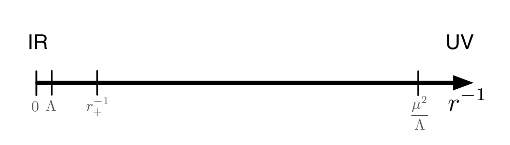
One reason that the re-expansion is technically useful is that it moves the logarithms of $r$ from the denominator in (20) to the numerator in (26). This is again familiar from QCD. To any fixed order in perturbation theory, logarithms of the scale in the renormalisation flow of the coupling will only appear in the numerator. However, because we know that the QCD coupling is asymptotically free, these logarithms must be resummed into the denominator so that the coupling flows to zero in the UV. Our original expansions (20) are the resummed expressions, while (26) has reintroduced a perturbation theory in the marginally relevant coupling by working at a scale $\mu$ which is much higher than the dynamically generated scale $\Lambda$. Similarly, at temperatures $T\gg\Lambda^{2}$ we will find that the deformation can be treated perturbatively.

Before moving on to discuss holographic renormalisation we briefly recall the physical role of relevant deformations in a weakly coupled realisation of $z=2$ Lifshitz criticality and a difference with the present strongly coupled case. The critical Lifshitz action considered in [14, 15, 16] is, up to ‘instanton’ terms and a marginally irrelevant coupling,

$$S_{\text{Lif}}={\textstyle{1\over 2}}\int d\tau d^{2}x\left((\partial_{\tau}\phi)^{2}+\tilde{K}(\nabla^{2}\phi)^{2}\right)\,.$$

(30)

This theory clearly has a $z=2$ scale invariance. The above action admits a relevant deformation by the term $\rho(\nabla\phi)^{2}$. If $\rho$ is positive then the theory flows to a Lorentz invariant theory in the IR. This is very analogous to the renormalisation group flow found numerically in [9] and that we are investigating in more depth in this paper. The difference between the two theories is that in the strongly coupled theory with a holographic dual, the natural deformation is marginally relevant rather than simply relevant as in the weakly coupled case. If $\rho$ is negative then one obtains a ‘tilted’ phase for the ‘height field’ $\phi$, i.e. an expectation value for $\nabla\phi$, that spontaneously breaks spatial isotropy. The Lifshitz theory (30) is then understood as the quantum critical theory separating tilted and untilted phases at zero temperature. In this paper we are only investigating the approach to criticality from one phase. We hope our results will provide a framework for a holographic realisation of the full quantum phase transition.

While we expect our bulk theory to be dual to a field theory with the same scaling symmetry as the above theory (30), we do not expect it to be dual to a theory with such a simple Lagrangian with a single scalar field. In the present paper we will not attempt to construct the dual field theory. Rather it will suffice to point out that there is a natural family of theories that has the counter-part of a matrix large $N$ limit. Generalisations of this theory are candidates for the field theory dual to the bulk theory discussed in the present paper. To motivate the existence of such a large $N$ theory, it will be illuminating to rewrite the Lagrangian (30) in the following way. Recall that a scalar is dual to a one-form in (2+1)-dimensions. Writing

$$\star d\phi=d{\bf A}\;,$$

the above Lagrangian is transformed into

$$S_{\text{Lif}}={\textstyle{1\over 2}}\int d\tau d^{2}x\left(|{\bf B}|^{2}+\tilde{K}|\nabla\times{\bf E}|^{2}\right)\,.$$

The $SU(N)$, $SO(N)$, $Sp(N)$ generalisations of the above $U(1)$ Lagrangian have been constructed in [28] and it would be interesting to establish the possible duality between such theories and the various bulk theories, e.g. [9, 29], which produce the Lifshitz spacetime (5) as a solution.

Using the equations of motion (12) it is possible to show that the bulk action (2) evaluated on-shell can be written as the integral of a total derivative and hence becomes a boundary term. Specifically, the Euclidean on-shell action gives the semiclassical free energy density

$${\cal F}_{E}=-\frac{1}{2}\left(\frac{\ell}{\kappa}\right)^{2}\lim_{r\to 0}\sqrt{f}rp^{\prime}\,.$$

(31)

By density we mean the density per unit boundary volume. That is, the free energy is $F=\int d^{2}x\,{\cal F}$, with no integral over the Euclidean time circle.

Before evaluating this action, we will need to add the boundary action and counterterms. Firstly there is the usual Gibbons-Hawking term required for the desired variational principle, which in Euclidean space evaluates to

$${\cal F}_{\text{G-H}}=\frac{1}{\kappa^{2}}\lim_{r\to 0}\sqrt{\gamma}\,K=\left(\frac{\ell}{\kappa}\right)^{2}\lim_{r\to 0}r(\sqrt{f}p)^{\prime}\,,$$

(32)

where $\gamma_{ab}$ is the induced metric on the boundary and $n^{\mu}\partial_{\mu}$ is an outward-pointing unit vector to the boundary which defines the extrinsic curvature $K_{\mu\nu}=-\nabla_{(\mu}n_{\nu)}$. The bulk and Gibbons-Hawking terms do not lead to a finite on-shell action, and therefore boundary counterterms are required to render the theory well defined.

There has been some confusion in the literature over the correct holographic renormalisation of asymptotically Lifshitz solutions to Einstein-Proca theory. The physics seems clear: the solutions describe two deformations of the Lifshitz theory by the operators $T^{tt}$ and $J^{t}$ and their corresponding expectation values. As neither of these operators appear to be irrelevant, they do not destroy the UV definition of the theory. Therefore we should be able to consistently describe the physics of all of these modes. It becomes a question of finding the correct boundary counterterms.

The approach we take is similar to [29]. In some regards our situation will be easier than the situation in that paper, because the theory studied there leads to unusually slowly falling off modes¹¹ 1 Specifically, [29] have metric modes falling off like $r^{2}$ as opposed to $r^{4}$ in the coordinates (5). even without the marginally relevant operator. Just as in that work, in order to preserve boundary covariance, we would like to consider counterterms in the form of a power series in $A^{2}=A^{\mu}A_{\mu}$. See [19] for an alternative choice of counterterms involving the combination $\sqrt{A^{\mu}A_{\mu}}$, which does not seem to generalise straightforwardly to include the marginally relevant deformation. As we will explain in more detail shortly, it turns out that just three such terms, $\sqrt{\gamma}(\tilde{c}_{0}+\tilde{c}_{1}A^{2}+\tilde{c}_{2}A^{4})$, are enough to render all the physical quantities of interest to us finite. The complication due to the marginally relevant deformation is that the coefficients $\{\tilde{c}_{i}\}$ become functions of $\log\Lambda r$.

Consider the following boundary counterterms in the free energy density

	$\displaystyle{\cal F}_{\text{c.t.}}$	$\displaystyle=$	$\displaystyle\frac{1}{2\ell\kappa^{2}}\lim_{r\to 0}\sqrt{\gamma}\sum_{n=0}^{2}c_{n}\left(-\frac{\kappa^{2}}{g^{2}}A^{2}-\frac{1}{2}\right)^{n}$		(33)
		$\displaystyle=$	$\displaystyle\frac{1}{2}\left(\frac{\ell}{\kappa}\right)^{2}\lim_{r\to 0}\sqrt{f}p\sum_{n=0}^{2}c_{n}(k^{2}-{\textstyle{1\over 2}})^{n}\,.$

We chose to write the series in this form for convenience, since $-\frac{\kappa^{2}}{g^{2}}A^{2}-\frac{1}{2}=0$ when evaluated on the Lifshitz solution. We will shortly write down the coefficients $\{c_{i}\}$ that make the total semiclassical free energy density

$${\cal F}={\cal F}_{\text{E}}+{\cal F}_{\text{G-H}}+{\cal F}_{\text{c.t.}}=\frac{1}{2}\left(\frac{\ell}{\kappa}\right)^{2}\lim_{r\to 0}\sqrt{f}p\left(\frac{rf^{\prime}}{f}+\frac{rp^{\prime}}{p}+\sum_{n=0}^{2}c_{n}(k^{2}-{\textstyle{1\over 2}})^{n}\right)\,,$$

(34)

finite.

Besides rendering the on-shell action finite, the counterterms should also lead to a well-defined variational problem and in particular finite on-shell expectation values and charges obtained by variation of the action with respect to boundary fields. Naïvely, following the usual procedure we would write the on-shell variation as

$$\delta{\cal F}=\frac{\sqrt{\gamma}}{2}\tau^{ab}\delta\gamma_{ab}+{\cal J}^{a}\delta A_{a}\;,$$

(35)

but some care is needed in the present case.

As shown in [30] in the more established AdS/CFT context, the usual charge defined by $\int d^{2}x\sqrt{\sigma}\xi_{a}k_{b}\tau^{ab}$, where $\xi^{a}\partial_{a}$ is a boundary Killing vector, $\sqrt{\sigma}=\sqrt{\gamma_{xx}\gamma_{yy}}$ is the spatial volume element and $k^{a}\partial_{a}$ is the unit normal to the boundary Cauchy surface, say $t=\text{const.}$, is not conserved when non-scalar matter fields are present. Instead, following [30, 19], when defining the energy-momentum tensor we should hold fixed the matter fields in the boundary vielbein frame, defined by the usual relation

$$\gamma_{ab}=\eta_{\hat{a}\hat{b}}e_{a}^{\hat{a}}e_{b}^{\hat{b}}\quad,\quad\eta=\text{diag}(\pm 1,1,1)\;,$$

(36)

where we have used the indices $a,b,...$ to denote the local coordinates on the boundary and the hatted indices to denote the local tangent space coordinates. The boundary stress tensor ${\cal T}^{ab}$ is then given by

$$\delta{\cal F}={\sqrt{\gamma}}\,{\cal T}^{a}_{\;\;\;\hat{a}}\,\delta e_{a}^{\hat{a}}+{\cal J}^{\hat{a}}\delta A_{\hat{a}}\,,\qquad{\cal T}^{ab}={\cal T}^{a}_{\;\;\;\hat{a}}e^{b\hat{a}}\;.$$

(37)

A short computation shows that

$${\cal T}^{ab}=\tau^{ab}+\frac{1}{\sqrt{\gamma}}\,{\cal J}^{(a}A^{b)}\,,$$

(38)

where the bracket denotes symmetrisation of indices. In particular, the energy density is given by

$${\cal E}=\sqrt{\sigma}\,k_{a}\,\xi_{b}\,{\cal T}^{ab}=\sqrt{\gamma}\,\tau^{t}{}_{t}+{\cal J}^{t}A_{t}\,.$$

(39)

While the ${\cal J}^{t}A_{t}$ term here is closely analogous to the standard chemical potential times charge term appearing in the canonical ensemble, we should remember that ${\cal J}^{t}$ in our system is not a conserved charge.

Taking the local frame to be

$$e^{\hat{t}}=e^{\hat{t}}_{a}dx^{a}=\sqrt{f}d\tau\;,\quad e^{\hat{x}}=\sqrt{p}\,dx\;,\quad e^{\hat{y}}=\sqrt{p}\,dy\;,$$

(40)

the quantities of particular interest can be computed to give

	$\displaystyle\tau^{ab}$	$\displaystyle=$	$\displaystyle\frac{2}{\sqrt{\gamma}}\frac{\delta{\cal F}}{\delta\gamma_{ab}}=\frac{1}{\kappa^{2}}\left(K^{ab}-K\gamma^{ab}\right)$		(41)
		$\displaystyle+$	$\displaystyle\frac{1}{2\ell\kappa^{2}}\sum_{n=0}^{2}c_{n}\left(\gamma^{ab}\left(-\frac{\kappa^{2}}{g^{2}}A^{2}-\frac{1}{2}\right)^{n}+2n\frac{\kappa^{2}}{g^{2}}A^{a}A^{b}\left(-\frac{\kappa^{2}}{g^{2}}A^{2}-\frac{1}{2}\right)^{n-1}\right)\,,$		(42)

and

	$\displaystyle{\cal J}^{\hat{t}}$	$\displaystyle=$	$\displaystyle\sqrt{f}\frac{\delta{\cal F}}{\delta A_{t}}=\frac{1}{g}\frac{\ell}{\kappa}\lim_{r\to 0}\sqrt{f}p\left(\frac{r(\sqrt{f}k)^{\prime}}{\sqrt{f}}+k\sum_{n=0}^{2}n\,c_{n}(k^{2}-{\textstyle{1\over 2}})^{n-1}\right)$		(43)
		$\displaystyle=$	$\displaystyle\frac{1}{g}\frac{\ell}{\kappa}\lim_{r\to 0}\sqrt{f}p\left(-\frac{1}{2}x+k\sum_{n=0}^{2}n\,c_{n}(k^{2}-{\textstyle{1\over 2}})^{n-1}\right)\;,$

and all other ${\cal J}^{\hat{a}}=0$. We have used the equation of motion (16) to obtain the second line of the previous equation. Putting these expressions together, we obtain

$${\cal E}=\left(\frac{\ell}{\kappa}\right)^{2}\lim_{r\to 0}\sqrt{f}p\left(\frac{rp^{\prime}}{p}-\frac{xk}{2}+\frac{1}{2}\sum_{n=0}^{2}c_{n}\,(k^{2}-{\textstyle{1\over 2}})^{n}\right)\;.$$

(44)

It will be very useful to note that the above expression for the energy density is related to the free energy in a simple way. Observe that

$\displaystyle\sqrt{f}p\left(\frac{rp^{\prime}}{p}-\frac{xk}{2}+\frac{1}{2}\sum_{n=0}^{2}c_{n}\,(k^{2}-{\textstyle{1\over 2}})^{n}\right)=\frac{1}{2}\sqrt{f}p\left(\frac{rf^{\prime}}{f}+\frac{rp^{\prime}}{p}+\sum_{n=0}^{2}c_{n}(k^{2}-{\textstyle{1\over 2}})^{n}\right)+K\;,$

(45)

where $K$ is the RG-invariant quantity we found in (19). Evaluating both sides in the UV ($r\to 0$) and using (44) and (34) leads to the simple relationship

$${\cal E}={\cal F}+\left(\frac{\ell}{\kappa}\right)^{2}\,K\;.$$

(46)

As we shall see later, this gives exactly the ‘integrated first law of thermodynamics’ when considering a black hole solution. Finally we can easily compute the pressure and find ${\cal P}=-\sqrt{\gamma}\tau_{\;\;x}^{x}=-{\cal F}$ as expected on general thermodynamic grounds. The off-diagonal components such as ${\cal T}^{t}_{\;\;x}={\tau}^{t}_{\;\;x}$ vanish on our solution.

As we have implied in the preceding discussion, in order to renormalise the on-shell action we will need three boundary terms given by three non-vanishing coefficients $c_{0},c_{1},c_{2}$. It turns out that instead of being constant, they are series in $\frac{1}{\log(\Lambda r)}$, with $r$ understood to be evaluated at a small cutoff value. This explicit dependence of the boundary counterterms on the cutoff is expected: the marginally relevant perturbation of the theory breaks scaling invariance at any fixed scale. This breaking of the scaling symmetry can be viewed as a conformal anomaly Ê[31]. However, scale invariance should be recovered in the strict $r\to 0$ limit, or equivalently the $\Lambda\to 0$ limit, and hence we can expect inverse powers of $\log\Lambda r$ to appear. Imposing finiteness of the free energy and energy densities we find

	$\displaystyle c_{0}$	$\displaystyle=$	$\displaystyle 6-\frac{8}{3\log^{2}(r\Lambda)}+\frac{65+120\log(-\log(r\Lambda))}{9\log^{3}(r\Lambda)}+\dotsi\,,$
	$\displaystyle c_{1}$	$\displaystyle=$	$\displaystyle 2+\frac{16}{3\log(r\Lambda)}+\frac{-91-120\log(-\log(r\Lambda))}{9\log^{2}(r\Lambda)}+\dotsi\,,$		(47)
	$\displaystyle c_{2}$	$\displaystyle=$	$\displaystyle-\frac{5}{3}+\frac{35}{9\log(r\Lambda)}+\frac{a-\frac{175}{18}\log(-\log(r\Lambda))}{\log^{2}(r\Lambda)}\;,$

where the ellipses again denote terms suppressed by extra factors of $\log(-\log\Lambda r)/\log\Lambda r$ or $1/\log\Lambda r$. A few remarks about these coefficients are in order. Firstly, notice that the first two coefficients are given in terms of infinite series, while the series expansion of the third coefficient terminates at $1/\log^{2}(\Lambda r)$. This can be understood in the following way. Observe that the divergences of the free energy and energy before renormalisation are both given in terms of $r^{-4}$ multiplied by an infinite series in $1/\log\Lambda r$, plus a finite number of divergent terms of the form $\log^{n}(\Lambda r)$ for some positive integer $n$. Hence we have altogether two infinite series and a few extra terms which need to be cancelled by the counterterms. Unsurprisingly, they are exactly cancelled by counterterms given by two infinite series and three more terms. Relatedly, there is an ambiguity in the final counterterm given by a real number denoted by $a$ in the above equation. This ambiguity does not afflict any of the thermodynamical quantities we shall study later. Nevertheless it does represent an ambiguity in the quantity ${\cal J}^{\hat{t}}$, which reflects the extent to which the system reacts upon changing the boundary (i.e. background) value of the Proca field $A_{\hat{t}}$. Such ambiguities are physical and common in the presence of logarithmically running couplings. It is also possible to add more subleading terms in the series for $c_{2}$, but these terms will not affect our results for ${\cal F},{\cal E}$ or ${\cal J}^{\hat{t}}$. Finally, it is also possible to add higher power counterterms such as $c_{3}(k^{2}-{\textstyle{1\over 2}})^{3}$. Nevertheless we shall make the above minimal choice which will be sufficient for our purposes.

After incorporating the appropriate counterterms given by (33) and (47), we obtain the following finite expressions for the physical quantities in terms of the parameters $\alpha,\beta$ in our expansions (20):

	$\displaystyle{\cal F}$	$\displaystyle=$	$\displaystyle\left(\frac{\ell}{\kappa}\right)^{2}\frac{\sqrt{2}}{9}\left(-5\beta+6\alpha\right)\,,$
	$\displaystyle{\cal E}$	$\displaystyle=$	$\displaystyle-\left(\frac{\ell}{\kappa}\right)^{2}\frac{\sqrt{2}}{9}\left(7\beta+6\alpha\,\right)\,,$		(48)
	$\displaystyle{\cal J}^{\hat{t}}$	$\displaystyle=$	$\displaystyle\frac{1}{g}\frac{\ell}{\kappa}\left(\frac{27}{703}+2a\right)\beta\;.$

From here we see that evaluated on the pure Lifshitz solution we have

$${\cal E}={\cal F}={\cal J}^{\hat{t}}=0\,.$$

Furthermore, recall that we have an RG-invariant quantity (19) which can be written in terms of the parameters $\alpha,\beta$ as

$$K=-\frac{1}{2}\sqrt{f}p\Big(-q+m+k\,x\Big)=-\frac{2\sqrt{2}}{9}\left(\beta+6\alpha\right)\;,$$

(49)

consistent with the relation (46) between the quantities ${\cal E}$, ${\cal F}$ and $K$.

Several works have studied black holes in Einstein-Proca theory for various values of $z$, e.g. [18, 22, 23, 24]. As we noted above, these studies focused on the quantum critical theory and tuned the marginally relevant deformation to zero. We will begin similarly to those studies, by expanding the (planar) black hole solution near the horizon, and then numerically integrating outwards towards the boundary. Since we have now learned how to analyze solutions which contain the marginally relevant mode at the boundary, we will be able to explore the energetics of these black objects for a family of black holes with different fluxes.

References

- [1] A. Altland and B. Simons, “Condensed matter field theory,”. Cambridge, UK: Univ. Pr. (2006) 624 p.
- [2] S. Sachdev, Quantum phase transitions. Cambridge University Press, UK, 1999.
- [3] J. A. Hertz, “Quantum critical phenomena,” Phys. Rev. B14 (1976) 1165–1184.
- [4] J. M. Maldacena, “The large N limit of superconformal field theories and supergravity,” Adv. Theor. Math. Phys. 2 (1998) 231–252, arXiv:hep-th/9711200.
- [5] S. A. Hartnoll, “Lectures on holographic methods for condensed matter physics,” 0903.3246.
- [6] C. P. Herzog, “Lectures on Holographic Superfluidity and Superconductivity,” J. Phys. A42 (2009) 343001, arXiv:0904.1975 [hep-th].
- [7] J. McGreevy, “Holographic duality with a view toward many-body physics,” arXiv:0909.0518 [hep-th].
- [8] S. A. Hartnoll, “Quantum Critical Dynamics from Black Holes,” arXiv:0909.3553 [cond-mat.str-el].
- [9] S. Kachru, X. Liu, and M. Mulligan, “Gravity duals of lifshitz-like fixed points,”Phys.Rev.D 78:106005,2008 (Aug., 2008) , 0808.1725.
- [10] A. Adams, A. Maloney, A. Sinha, and S. E. Vazquez, “1/N Effects in Non-Relativistic Gauge-Gravity Duality,” JHEP 03 (2009) 097, arXiv:0812.0166 [hep-th].
- [11] M. Taylor, “Non-relativistic holography,” 0812.0530.
- [12] A. Proca, “Sur la thèorie ondulatoire des électrons positifs et nègatifs,” Journal de Physique et le Radium 7 (1936) 347.
- [13] D. S. Rokhsar and S. A. Kivelson, “Superconductivity and the Quantum Hard-Core Dimer Gas,” Phys. Rev. Lett. 61 (1988) 2376–2379.
- [14] A. Vishwanath, L. Balents, and T. Senthil, “Quantum criticality and deconfinement in phase transitions between valence bond solids,” cond-mat/0311085.
- [15] E. Fradkin, D. A. Huse, R. Moessner, V. Oganesyan, and S. L. Sondhi, “On bipartite rokhsar-kivelson points and cantor deconfinement,” Phys. Rev. B 69, (2004) 224415, cond-mat/0311353.
- [16] E. Ardonne, P. Fendley, and E. Fradkin, “Topological order and conformal quantum critical points,” Annals Phys. 310 (2004) 493–551, cond-mat/0311466.
- [17] S. A. Hartnoll, J. Polchinski, E. Silverstein, and D. Tong, “Towards strange metallic holography,” arXiv:0912.1061 [hep-th].
- [18] G. Bertoldi, B. A. Burrington, and A. Peet, “Black Holes in asymptotically Lifshitz spacetimes with arbitrary critical exponent,” arXiv:0905.3183 [hep-th].
- [19] S. F. Ross and O. Saremi, “Holographic stress tensor for non-relativistic theories,” JHEP 09 (2009) 009, arXiv:0907.1846 [hep-th].
- [20] U. Gursoy and E. Kiritsis, “Exploring improved holographic theories for qcd: Part i,”JHEP 0802:032,2008 (July, 2007) , 0707.1324.
- [21] K. Skenderis, M. Taylor, and B. C. van Rees, “Topologically Massive Gravity and the AdS/CFT Correspondence,” JHEP 09 (2009) 045, arXiv:0906.4926 [hep-th].
- [22] R. B. Mann, “Lifshitz topological black holes,” 0905.1136.
- [23] U. H. Danielsson and L. Thorlacius, “Black holes in asymptotically lifshitz spacetime,”JHEP 0903:070,2009 (Dec., 2008) , 0812.5088.
- [24] G. Bertoldi, B. A. Burrington, and A. W. Peet, “Thermodynamics of black branes in asymptotically Lifshitz spacetimes,” arXiv:0907.4755 [hep-th].
- [25] P. Horava and C. M. Melby-Thompson, “Anisotropic Conformal Infinity,” arXiv:0909.3841 [hep-th].
- [26] M. Henneaux, C. Martinez, R. Troncoso, and J. Zanelli, “Asymptotically anti-de Sitter spacetimes and scalar fields with a logarithmic branch,” Phys. Rev. D70 (2004) 044034, arXiv:hep-th/0404236.
- [27] A. J. Amsel and D. Marolf, “Energy bounds in designer gravity,” Phys. Rev. D74 (2006) 064006, arXiv:hep-th/0605101.
- [28] P. Horava, “Quantum criticality and yang-mills gauge theory,” 0811.2217.
- [29] K. Balasubramanian and J. McGreevy, “An analytic lifshitz black hole,” 0909.0263.
- [30] S. Hollands, A. Ishibashi, and D. Marolf, “Counter-term charges generate bulk symmetries,” Phys.Rev. D 72 (2005) 104025, hep-th/0503105.
- [31] M. Henningson and K. Skenderis, “The holographic weyl anomaly,” JHEP 9807 (1998) 023, hep-th/9806087.