Inflation with Non-minimal Gravitational Couplings and Supergravity
Abstract:
We explore in the supergravity context the possibility that a Higgs scalar may drive inflation via a non-minimal coupling to gravity characterised by a large dimensionless coupling constant. We find that this scenario is not compatible with the MSSM, but that adding a singlet field (NMSSM, or a variant thereof) can very naturally give rise to slow-roll inflation. The inflaton is necessarily contained in the doublet Higgs sector and occurs in the -flat direction of the two Higgs doublets.
Keywords:
inflation, supersymmetry, supergravity1 Introduction
The idea that a large non-minimal coupling of scalar fields to gravity might play an important role in inflation is clearly worth exploring. (For an early example see Ref. [1]). In particular, there has been recent interest [2]-[11] in the economical possibility that the standard model (SM) Higgs can be the relevant scalar; the action is
| (1) |
where is the Ricci scalar, and is a dimensionless coupling constant, assumed positive, 11 1 Here, the action has been expressed in the Jordan frame; one may transform to the Einstein frame by a conformal transformation. and is the Lagrangian of the SM, generalized to a nontrivial background spacetime obtained by replacing the flat-space metric with the curved space metric Classically, for large enough values of and , viz.,
| (2) |
(where ), it transpires that the scalar potential is nearly flat and the standard slow-roll approximation is possible. The issue of whether this classical analysis remains valid as an effective quantum field theory for field values in the range Eq. (2) is a matter of debate at present. On the one hand, there are some [6, 7] who argue that, as an effective field theory, the full action Eq. (1) must include higher dimensional operators, such as so that one would expect the theory to work up to an energy scale which is far below the regime suggested by Eq. (2).
On the other hand, others argue the effective field theory works within the regime in Eq. (2) for a variety of reasons. One such argument [1, 4, 8, 9] is that loops involving virtual Higgs are suppressed because their propagators are modified from ordinary perturbation theory for large values of the Higgs field. The treatment of gravity as a classical background may also be challenged. One would normally expect that the feedback on the metric would become strong on scales of the order of but one may hope [1, 2] that, in some models, the the energy density associated with Higgs remains small compared to even for provided it is not very much larger, say On the other hand, Higgs-graviton scattering would seem to become strong or to violate unitarity for energies [6, 7]. We will not address this issue directly in this paper, but we will return to it again in our conclusions.
The occurrence of such non-minimal couplings of matter fields to the background curvature is a fact of life in the SM, because the notion of minimal coupling () is only valid classically. In quantum field theory, the renormalized runs, i.e, is a function of a scale parameter () for which is not a fixed point [12, 13]. Thus, the “minimal theory” is at best an approximation to cases where the contributions of terms like the term above may be neglected.
Whether or not perturbation theory remains viable in the scenario, the scales of interest are large compared to the electroweak unification scale, so that the SM becomes unnatural, suffering also other apparent shortcomings such as unsatisfactory grand unification and lack of a suitable Dark Matter candidate. The latter issue is addressed, for example, in Refs. [14, 15] by adding a singlet to the standard model. More attractive alternatives to the SM above the TeV-scale are supersymmetric extensions of SM, which overcome the three most glaring deficiencies of the SM mentioned. An obvious question is whether the inflationary scenario described above survives in such supersymmetric models, and, if so, what their properties are. In this paper, we shall consider the MSSM and a simple extension with an additional singlet field (NMSSM), with which we will assume the reader is familiar (for a review see Ref. [16]).
An outline of the remainder of this paper is as follows: in the next section, we review the standard form of supergravity and then consider the addition of a non-minimal interaction analogous to the above. In Section 3, we apply this formalism to the MSSM , following in Section 4 with the NMSSM. Section 5 contains an analysis of the slow roll parameters in the one successful scenario that we identified. In Section 6, we restate our conclusions and discuss issues for future work, commenting on some dramatic differences from the SM to be anticipated for radiative corrections resulting from supersymmetry.
2 Non-minimal couplings in supergravity
Although particle physics generally ignores gravity in generalizing to supersymmetry, its inclusion is mandatory in the present context. Thus, the natural starting point is not global supersymmetry but the modification of the Lagrangian for supergravity22 2 Our notation and conventions follow Wess and Bagger [17], and from now on we set . coupled to a multiplet of chiral superfields :
| (3) |
where is the vierbein multiplet, is the curvature multiplet containing the scalar curvature in its component, and is the superpotential. For our purposes, we will not need the explicit form of the gauge field contributions.
To extend Eq. (1) to the supersymmetric case we replace Eq. (3) by
| (4) |
where is quadratic in , with coefficients which are dimensionless coupling constants. We shall discuss examples below, but an immediate consequence of SUSY is that the gauge invariant function is a function of the chiral superfields only and not A second consequence is that, by the non-renormalization theorem, the various monomials in will (in a similar manner to those in the superpotential ) not be generated through radiative corrections if absent from the classical action (in contrast to the case of the SM from Eq. (1)).
The scalar potential in the Einstein frame for the theory defined by Eq. (3) is given by
| (5) | |||||
where , is the Kähler potential, and the -terms will be discussed below. We will take to have the canonical form
| (6) |
where
| (7) |
In Eq. (5), etc.
One can show that the effect of the non-minimal couplings on the scalar potential, generalising from Eq. (3) to Eq. (4), is simply to replace in Eq. (7) by
| (8) |
Let us turn to the -term. In general, this takes the form (for a simple group with gauge coupling )
| (9) |
where is associated with the kinetic energy of the gauge field and, therefore, must be a holomorphic function of , and where transform according to a representation of the gauge group. Noting that
| (10) |
by gauge invariance, and assuming for simplicity the canonical form , we find
| (11) |
Thus in the MSSM, the are
| (12) |
where and are the two Higgs doublets, and are the Pauli matrices.
The behavior of the potential depends in detail on the choice of superpotential , but we will be interested in directions in field space in which the potential is approximately constant for large values of the Higgs fields.
3 MSSM
Let us begin by considering the effect of Eq. (8) on the scalar potential for the MSSM. The unique possibility for in this case is
| (13) |
where is constant; and, dropping terms involving fields that do not appear in , the most general possibility for the superpotential is
| (14) |
where and are constants. So contains no dimensionless couplings. One cannot in general choose both and to be real; however, we will ignore this potential source of -violation in what follows, since, as we shall soon see, this case does not yield a suitable inflationary regime. Without loss of generality, we may choose
Let us calculate the potential in the electromagnetism-preserving direction
| (15) |
where we may assume are real. If, as usual, we define and we can then write
| (16) |
We shall be interested in the case when but so we must have to avoid a singularity in . Since we must take We find
| (17) |
where
| (18) |
It is easy to see that, for fixed in the regime
| (19) |
the potential is dominated by the -term,
| (20) |
except very near the -flat direction, more precisely, for It is clear, however, that slow-roll conditions (to be reviewed below) will not be satisfied in these circumstances, because
| (21) |
cannot be made small.
On the other hand, in the -flat direction where , both and vanish, and Thus, this is a minimum stable against fluctuations in Then, in the regime described in Eq. (19), we have
| (22) |
or for , . In either case, through negative values, and so is unsuitable for an inflationary scenario.
4 NMSSM
Evidently, the failure of this MSSM to emulate the result of a nonminimal coupling in the nonsupersymmetric case is because of the absence of a cubic term in the superpotential, leading to the absence (in the -flat direction) of an analog to the dimensionless self-interaction (Of course inclusion of the usual Yukawa cubic terms in would lead to quartic terms in , but we need quartic terms that contain only fields that occur in in order to produce a suitable flat potential). It is therefore natural to turn to the NMSSM, which clearly can provide a cure to this behavior. Thus we consider the superpotential
| (23) |
where is a gauge singlet. There are then two natural choices for , to wit
| (24) | |||||
| (25) |
Note that in the case of Eq. (24) we can choose both and to be real.
If we choose Eq. (24) and consider the case when is small but is large,
| (26) |
then we find
| (27) |
which, taking the the Eq. (19) limit, becomes
| (28) |
which is (of course) minimized for . For this value of , Eq. (27) gives
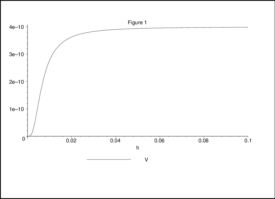
| (29) |
a smoothly increasing function of , precisely the behavior that we can expect to yield inflation. This is the supersymmetric analog of the model of Ref. [2]. We plot in Figure 1, for and .
On the other hand, if we choose Eq. (25) and small, then we find33 3 In principle, we cannot choose both and real. For our purposes, it is convenient to take real but possibly complex.
| (30) |
Writing we have
| (31) |
which in the limit gives
| (32) |
Thus for fixed , approaches a constant, but if then this constant is negative. If we choose in order to obtain then we see from Eq. (31) that as reduces, then increases, and we eventually encounter a pole in , when
| (33) |
Thus this case is not suitable for inflation.
5 Slow-roll analysis
Let us pursue the more promising case of Eq. (29) in more detail and calculate the slow-roll parameters. Evidently these relate to fluctuations and so we must consider the kinetic energies of the relevant fields. It is easy to show using Eq. (8) that in general the scalar kinetic energy takes the form
| (34) |
where is the vierbein and
| (35) |
Let us now briefly review the slow-roll paradigm (see for example Ref. [18]). Suppose the action that describes the inflaton takes the form
| (36) |
Then neglecting its spatial variation, the equation of motion for is
| (37) |
where
| (38) |
Then the slow-roll parameter is given by
| (39) |
where the latter approximation is valid if and can both be safely neglected in Eq. (37).
The number of -folds before inflation ends is given by
| (40) |
and the second slow-roll parameter is given by
| (41) |
In the slow-roll regime, and slow-roll ends when .
We now apply this formalism to the NMSSM doublet case. We first suppose that , that is we consider the -flat direction. From Eqs. (8), (15), (24), (34) we find that for large (as defined in Eq. (19)) the dominant contribution to the inflaton kinetic energy term is
| (42) |
Armed with this result we immediately obtain (given Eq. (19)) from Eqs. (39), (40) and (41) that
| (43) | |||||
| (44) | |||||
| (45) |
We see that the slow-roll conditions are satisfied given Eq. (19). Moreover it is easy to verify that the approximations made in neglecting and in Eq. (37) are well justified. The results are similar to those of Ref. [5]. For , and using as in Ref. [5], we obtain , in the neighborhood of the GUT scale.
Suppose that at large fixed . Might it be that the slow-roll conditions are satisfied with ? In fact it is easy to show that
| (46) |
from which one sees that as , . Thus we see that, unlike in the MSSM case, models with a sufficiently slow approach to the -flat direction might be entertained.
6 Conclusions
In conclusion, we have demonstrated that, in the presence of non-minimal gravitational interactions in the NMSSM, but not in the MSSM, there is contained in the Higgs sector a viable inflaton candidate, as in the SM. Although we have not yet completed an analysis of the running of the couplings in this model, we remarked earlier that the non-renormalization properties of SUSY and SUGRA models make the behavior of the non-minimal couplings different. In particular, unlike in the nonsupersymmetric case, the beta function for will therefore have a fixed point at It would be interesting to implement refinements taking into account renormalisation group evolution described (and debated) for the SM case in Refs. [2]-[11], and explore the consequences for the Higgs spectrum; in particular, perhaps in the MNMSSM [19] where the spectrum is more constrained.
Given that these calculations seem to be concerned with the dynamics in the region beyond the GUT scale, one question is whether the same sort of results can be obtain within supersymmetric GUTS [20]-[23] such as or Does inflation end somewhere below the (reduced) Planck scale but above the GUT scale ? Is the dynamics of inflation viable over such a relatively narrow range of energies as this?
The most important unanswered question is whether these calculations make sense from the point of view of effective quantum field theory. As we discussed, this is a point of controversy in the literature, and we hope to return to this issue in the future. It is partly a question of the range of scales over which perturbation theory can be used, and it is partly a question of just what is the expansion parameter. We certainly have assumed that it makes sense to use the nonpolynomial potential on energy scales in the Einstein frame associated with changes in the gravitational constant in the Jordan frame, where the action has the familiar polynomial form. Even if the arguments were correct that, in the SM, this model for inflation is unnatural, will the situation be improved as a result of supersymmetry? We leave this for future investigation.
Acknowledgements
DRTJ thanks KITP (Santa Barbara) for hospitality and financial support. This work was partially supported by the Royal Society through a collaboration grant, and by National Science Foundation under Grant No. PHY99-07949.
References
- [1] D. S. Salopek, J. R. Bond and J. M. Bardeen, Phys. Rev. D 40, 1753 (1989).
- [2] F. L. Bezrukov and M. Shaposhnikov, Phys. Lett. B 659 (2008) 703 [arXiv:0710.3755 [hep-th]].
- [3] A. O. Barvinsky, A. Y. Kamenshchik and A. A. Starobinsky, JCAP 0811, 021 (2008) [arXiv:0809.2104 [hep-ph]].
- [4] A. De Simone, M. P. Hertzberg and F. Wilczek, Phys. Lett. B 678, 1 (2009) [arXiv:0812.4946 [hep-ph]].
- [5] F. L. Bezrukov, A. Magnin and M. Shaposhnikov, Phys. Lett. B 675 (2009) 88 [arXiv:0812.4950 [hep-ph]].
- [6] C. P. Burgess, H. M. Lee and M. Trott, JHEP 0909, 103 (2009) [arXiv:0902.4465 [hep-ph]].
- [7] J. L. F. Barbon and J. R. Espinosa, Phys. Rev. D 79, 081302 (2009) [arXiv:0903.0355 [hep-ph]].
- [8] F. Bezrukov and M. Shaposhnikov, JHEP 0907, 089 (2009) [arXiv:0904.1537 [hep-ph]].
- [9] A. O. Barvinsky, A. Y. Kamenshchik, C. Kiefer, A. A. Starobinsky and C. Steinwachs, JCAP 0912, 003 (2009) [arXiv:0904.1698 [hep-ph]].
- [10] A. O. Barvinsky, A. Y. Kamenshchik, C. Kiefer, A. A. Starobinsky and C. F. Steinwachs, arXiv:0910.1041 [hep-ph].
- [11] N. Okada, M. U. Rehman and Q. Shafi, arXiv:0911.5073 [hep-ph].
- [12] I. Jack and H. Osborn, Nucl. Phys. B 249, 472 (1985).
- [13] See, for example, I. L. Buchbinder, S. D. Odintsov and I. L. Shapiro, “Effective action in quantum gravity,” Bristol, UK: IOP (1992) 413 p.
- [14] T. E. Clark, B. Liu, S. T. Love and T. ter Veldhuis, Phys. Rev. D 80, 075019 (2009) [arXiv:0906.5595 [hep-ph]].
- [15] R. N. Lerner and J. McDonald, arXiv:0909.0520 [hep-ph].
- [16] U. Ellwanger, C. Hugonie and A. M. Teixeira, arXiv:0910.1785 [hep-ph].
- [17] J. Wess and J. Bagger, Princeton, USA: Univ. Pr. (1992) 259 p
- [18] D. Baumann, arXiv:0907.5424 [hep-th].
- [19] C. Panagiotakopoulos and A. Pilaftsis, Phys. Rev. D 63 (2001) 055003 [arXiv:hep-ph/0008268].
- [20] S. Dimopoulos and H. Georgi, Nucl. Phys. B 193, 150 (1981).
- [21] L. E. Ibanez and G. G. Ross, Phys. Lett. B 105, 439 (1981).
- [22] M. B. Einhorn and D. R. T. Jones, Nucl. Phys. B 196, 475 (1982).
- [23] A. H. Chamseddine, R. L. Arnowitt and P. Nath, Phys. Rev. Lett. 49, 970 (1982).