Asymptotics of Lagged Fibonacci Sequences

Let $k>1$ be an integer and consider “lagged” Fibonacci type sequences

$$a_{k}(n)=a_{k}(n-1)+a_{k}\left(\left\lfloor\frac{n}{k}\right\rfloor\right)$$

(1)

with initial value

$$a_{k}(0)=1\,.$$

(2)

These “almost linear recurrence” has many interesting arithmetical properties [1]. The value $a_{k}(n)$ equals the number of $k$-ary partitions of $kn$, and the corresponding sequences are listed in the OEIS as A000123, A005704, A005705 and A005706 for $k=2,3,4,5$, respectively. In this contribution we will study the asymptotical behavior of the ratio

$$c_{k}(n)=\frac{a_{k}(kn)}{a_{k}(n)}\,\frac{\ln n}{n}\,.$$

(3)

The OEIS entry for A000123 quotes a conjecture due to Benoit Cloitre, claiming that

$$\lim_{n\to\infty}c_{k}(n)=\text{const.}=1.63\ldots\,.$$

(4)

The same conjecture (but with $\text{const.}=1.64\ldots$) appears for the related sequence A033485. We will prove that the essential part of the conjecture (existence of the limit) is true, but that its numerical part is incorrect. In particular, we will apply a classical result of de Bruijn [2] to prove that

$$\lim_{n\to\infty}c_{k}(n)=k\ln k\,.$$

(5)

Note that $2\ln 2=1.386\ldots$, which differs significantly from the value in (4).

In the second part we will discuss the rate of convergence of $c_{k}(n)$. It turns out that this rate is so slow that straightforward numerical measurements of $c_{k}(n)$ cannot be used for an accurate measurement of $c_{k}(\infty)$. This may explain the inaccurate numerical value in (4). It turns out that another classical result on the asymptotics of $a_{k}(n)$ due to K. Mahler [3] can be used as a device for an accurate numerical determination of $c_{k}(n)$ all the way to the asymptotic regime.

In the final part we will discuss the connection between the two asymptotic formulas of de Bruijn and Mahler.

Using an integral representation (Mellin transformation) of the generating function for $a_{k}(n)$ and a saddle point integration, de Bruijn [2] showed that

	$\displaystyle\ln a_{k}(n)=$	$\displaystyle\frac{1}{2\ln k}(\ln n-\ln\ln n)^{2}+\left(\frac{1}{2}+\frac{1}{\ln k}+\frac{\ln\ln k}{\ln k}\right)\ln n-\left(1+\frac{\ln\ln k}{\ln k}\right)\ln\ln n$		(6)
		$\displaystyle+\left(1+\frac{\ln\ln k}{2\ln k}\right)\ln\ln k-\frac{1}{2}\ln(2\pi)+\psi_{k}\left(\log_{k}\Big(\frac{n}{\log_{k}n}\Big)\right)+\mathcal{O}\left(\frac{\ln^{2}\ln n}{\ln n}\right)\,,$

where $\psi_{k}$ is a periodic function with period $1$,

$$\psi_{k}(x)=\sum_{j=-\infty}^{\infty}\alpha_{j}(k)\mathrm{e}^{2\pi ijx}\,.$$

(7)

The Fourier coefficients are

$$\alpha_{j}(k)=\frac{1}{\ln k}\,\Gamma\left(\frac{2\pi ij}{\ln k}\right)\,\zeta\left(1+\frac{2\pi ij}{\ln k}\right)\qquad(j\neq 0)$$

(8)

and

$$\alpha_{0}(k)=\frac{1}{\ln k}\left(-\gamma_{1}-\frac{1}{2}\gamma^{2}+\frac{1}{12}\pi^{2}+\frac{1}{12}\ln^{2}k\right)\,,$$

(9)

where $\gamma=0.5772156649\ldots$ is the Euler constant and $\gamma_{1}=-0.0728158454\ldots$ is the first Stieltjes constant.

The Fourier series for $\psi_{k}(x)$ converges absolutely and uniformely because the coefficients $\alpha_{j}(k)$ decay fast enough:

$$|\Gamma(it)|=\mathcal{O}(|t|^{-\frac{1}{2}}\mathrm{e}^{-\frac{1}{2}\pi|t|})$$

(10)

and

$$|\zeta(1+it)|=\mathcal{O}(\ln|t|)\,.$$

(11)

Plugging (6) into (3) provides us with

$$\ln c_{k}(n)=\ln(k\ln k)+\Delta\psi_{k}(n)+\mathcal{O}\left(\frac{(\ln\ln n)^{2}}{\ln n}\right)\,,$$

(12)

where

$$\Delta\psi_{k}(n)=\psi_{k}\left(\log_{k}\Big(\frac{n}{\log_{k}n}\Big)-\log_{k}\Big(1+\frac{1}{\log_{k}n}\Big)\right)-\psi_{k}\left(\log_{k}\Big(\frac{n}{\log_{k}n}\Big)\right)\,.$$

(13)

Intuitively, $\Delta\psi_{k}(n)$ should vanish for $n\to\infty$, but to be sure we need to investigate the Fourier series for $\psi_{k}$ in more detail. In particular, we have

	$\displaystyle|\Delta\psi_{k}(n)|$	$\displaystyle=\left|\sum_{j=-\infty}^{\infty}\alpha_{j}(k)\exp\left(2\pi ij\log_{k}\Big(\frac{n}{\log_{k}n}\Big)\right)\,\left(\exp\left(-2\pi ij\log_{k}\Big(1+\frac{1}{\log_{k}n}\Big)\right)-1\right)\right|$
		$\displaystyle\leq\sum_{j=-\infty}^{\infty}|\alpha_{j}(k)|\,\left|\exp\left(-2\pi ij\log_{k}\left(1+\frac{1}{\log_{k}n}\right)\right)-1\right|$
		$\displaystyle\leq 2\pi\sum_{j=-\infty}^{\infty}|j\,\alpha_{j}(k)|\,\left|\log_{k}\left(1+\frac{1}{\log_{k}n}\right)\right|\,.$

In the last line we have used the inequality

$$|\mathrm{e}^{ix}-1|\leq|x|\qquad(x\in\mathbb{R})\,.$$

(14)

Now because of (10) and (11) we know that $\sum_{j}|j\alpha_{j}(k)|<\infty$, and hence

$$\Delta\psi_{k}(n)=\mathcal{O}(1/\log_{k}n)\,.$$

(15)

This concludes our proof of (5).

The recurrence (1) appears in the analysis of the Karmarkar-Karp differencing algorithm for number partitioning [4]. In this context we learned that the convergence to the asymptotic regime can be extremely slow. We will see that this is also true when we try to probe the asymptotics of $c_{k}(n)$ numerically.

To calculate $c_{k}(n)$, we need $a(kn)$ and $a(n)$, but because of

$$a_{k}(kn)=a_{k}(n)+k\sum_{j=0}^{n-1}a_{k}(j)\,,$$

(16)

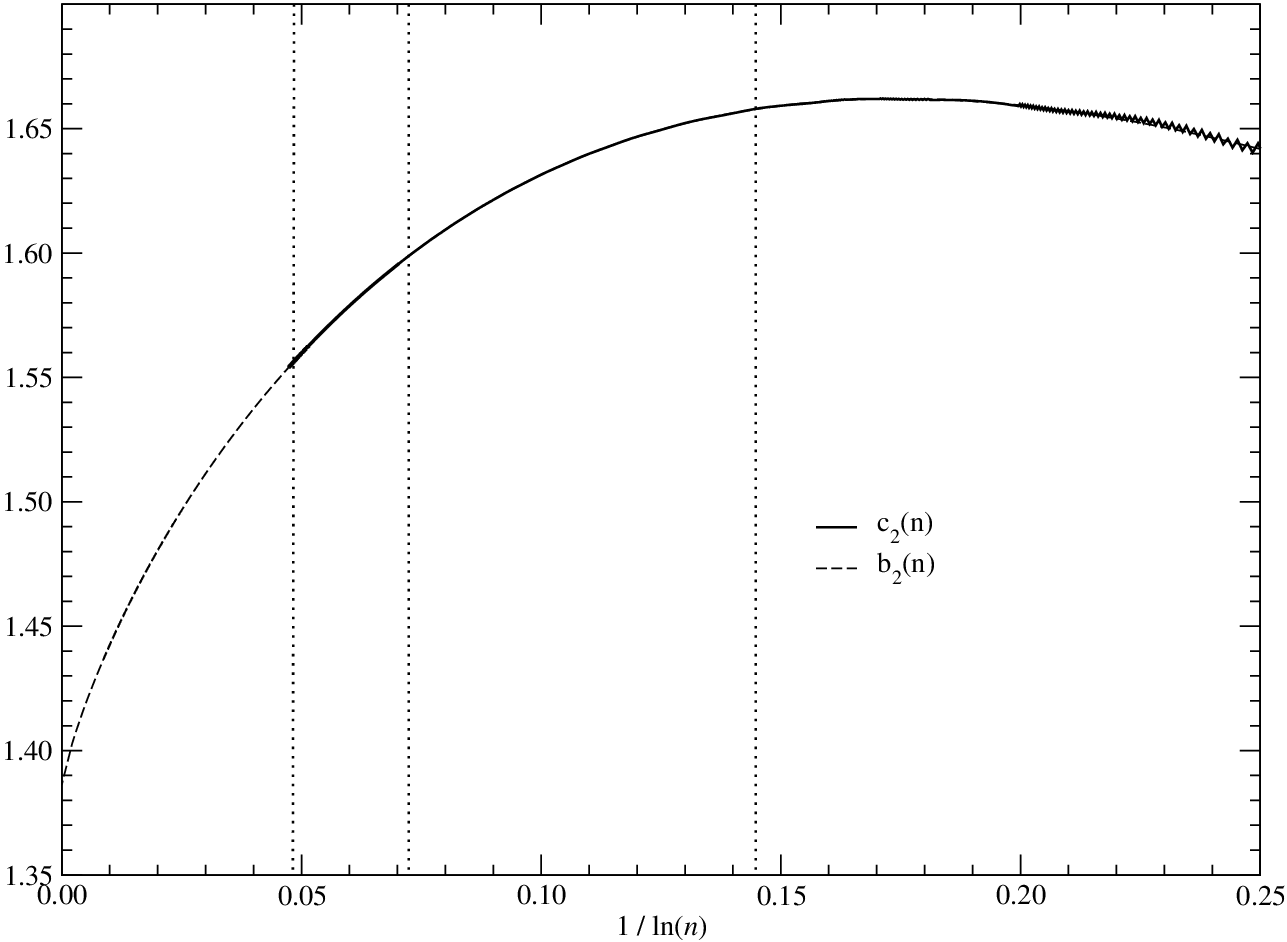
the value of $a_{k}(n)$ plus the sum of the preceeding terms is sufficient. The bottleneck for calculating $a_{k}(n)$ is memory, not CPU time, since $n(1-1/k)$ values must be stored to compute $a_{k}(n)$. We used the Chinese Remainder Theorem to keep the individual numbers small and managed to calculate $c_{2}(n)$ for $n$ up to $3\cdot 10^{9}$ on a PC with $4$ GByte of memory. As Fig. 1 shows, even these data are insufficient to extrapolate to the true asymptotic value. Numerical calculations that stop at even smaller values of $n$ may easily misguide an extrapolation to $c_{k}(\infty)$.

In order to evaluate $c_{k}(n)$ for much larger values of $n$, we resort to another asymptotic result. In 1940, Mahler [3] showed that

$$a_{k}(n)=\mathrm{e}^{\phi_{k}(n)}\sum_{j=0}^{\infty}\frac{n^{j}}{k^{\binom{j}{2}}j!}\equiv\mathrm{e}^{\phi_{k}(n)}\,S_{k}(n)$$

(17)

where $\phi_{k}(n)=O(1)$. The idea is to replace the numerical evaluation of $a_{k}(n)$ by the numerical evaluation of the sum $S_{k}(n)$. Note that $S_{k}(n)$ can be evaluated for very large values of $n$ using a computer algebra system. A discrepancy in this approach arises from the unknown function $\phi_{k}$. Albeit asymptotically bounded, it can introduce large errors for finite values of $n$.

It was already noticed by Fröberg [5], that $\phi_{k}$ oscillates with a small (and decaying) amplitude around a constant value. We used our extensive data for $a_{k}(n)$ to look more closely at

$$\phi_{k}(n)\equiv\ln a_{k}(n)-\ln\sum_{j=0}^{\infty}\frac{n^{j}}{k^{\binom{j}{2}}j!}\,.$$

(18)

As can be seen from Figure 2, the amplitude of $\phi_{2}$ is smaller than $10^{-4}$ for $n>10^{4}$, and it is slowly, but monotonically decaying. The constant around which $\phi_{k}$ oscillates will cancel in the ratio

$$\frac{a_{k}(kn)}{a_{k}(n)}=\mathrm{e}^{\phi_{k}(kn)-\phi_{k}(n)}\,\frac{S_{k}(kn)}{S_{k}(n)}$$

Hence the error is bounded by the small amplitude. This is confirmed by the numerical data, see Table 1. Even for $n=100$, the error in $c_{2}(n)$ is only in the fourth decimal.

This observation tells us that we can use

$$b_{k}(n)=\frac{S_{k}(kn)}{S_{k}(n)}\,\frac{\ln n}{n}$$

(19)

as an excellent approximation to $c_{k}(n)$. Since $b_{k}(n)$ can be evaluated for very large values of $n$, like $n=2^{1000}$ and beyond, we can use $b_{k}(n)$ to bridge the gap between the numerically accessible $c_{k}(n)$ and $c_{k}(\infty)$ (Figure 1).

The results of de Bruijn (6) and Mahler (17) have to match, i.e., we know that $\phi_{k}(n)+\ln S_{k}(n)$ equals the right hand side of (6). A saddle-point expansion of $S_{k}(n)$ (see (36) in the Appendix) reveals that the leading terms of $\ln S_{k}(n)$ equal the leading terms in (6). The remaining terms yield

$$\phi_{k}(n)=\Psi_{k}\left(\log_{k}\Big(\frac{n}{\log_{k}n}\Big)\right)+\left(1+\frac{\ln\ln k}{\ln k}\right)\ln k-\frac{1}{2}\ln(2\pi)+\frac{(\ln k+2\ln\ln k)^{2}}{8\ln k}+\mathcal{O}\left(\frac{\ln^{2}\ln n}{\ln n}\right)\,.$$

(20)

In particular, we see that asymptotically $\phi_{k}$ oscillates around a value

$$\left(1+\frac{\ln\ln k}{\ln k}\right)\ln k-\frac{1}{2}\ln(2\pi)-\frac{(\ln k+2\ln\ln k)^{2}}{8\ln k}+\alpha_{0}(k)\,,$$

(21)

with $\alpha_{0}(k)$ from (9). For $k=2$, this constant is $-0.079793025\ldots$ (see Figure 2), in perfect agreement with the numerical results of Fröberg [5].

The asymptotic amplitude of $\phi_{k}$ is very small, as can be seen by evaluating the coefficients (8), see Table 2. Hence we know that the oscillation in Figure 2 will eventually decay to an amplitude of size $10^{-6}$. We have calculated a few more minima and maxima of $\phi_{2}$ to check this decay. Figure 3 shows the result. The extrapolation of the numerical data gives very accurate result for the constant $-0.079793025\ldots$ as well as the right order of magnitude ($10^{-6}$) of the remanent amplitude.

We thank Sebastian Mingramm for providing us with the numerical values for $a_{2}(n)$ for $n>10^{7}$. SB thanks the Institut für Theoretische Physik at Otto-von-Guericke University in Magdeburg for its hospitality during the preparation of this manuscript and gratefully acknowledges support from a Fulbright-Kommision grant and from the U.S. National Science Foundation through grant number DMR-0812204.

Here, we evaluate the asymptotic behavior of the sum

$\displaystyle S_{k}(n)=\sum_{j=0}^{\infty}\frac{n^{j}}{j!\,k^{\frac{j(j-1)}{2}}}\qquad(n\to\infty)$

(22)

using a saddle-point expansion. Following Ref. [6] (pp. 304), we define $\Phi_{j}=\ln a_{j}$ for the summand $a_{j}$. The finite-difference condition $D\Phi_{j}=\Phi_{j}-\Phi_{j-1}=0$ determines the maxima, i. e. we need to find the $j_{0}$-term(s) of the sum with $a_{j_{0}}/a_{j_{0}-1}\sim 1$. Applied to Eq. (22), we obtain

$\displaystyle\eta\left[j_{0}+\Delta_{j}-1+\log_{k}\left(j_{0}+\Delta_{J}\right)\right]$

$\displaystyle\sim$

$\displaystyle 1$

(23)

where we use the abbreviations

$\displaystyle\eta=\frac{1}{\log_{k}n}$

$\displaystyle=$

$\displaystyle\frac{\ln k}{\ln n}$

(24)

and a non-integer offset $0\leq\Delta_{j}\leq 1$ on the integer location $j_{0}$ of the saddlepoint, which we will need to attain the continuum limit for this $n$-dependent (“moving”) saddle point [6]. For $n\to\infty$, $\eta\to 0$ and in that limit we find from Eq. (23) for the saddle-point location by peeling off layer-by-layer:

	$\displaystyle j_{0}$	$\displaystyle=$	$\displaystyle\frac{1}{\eta}+\log_{k}\eta+1-\Delta_{j}-\eta\frac{1+\log_{k}\eta}{\ln k}+\eta^{2}\frac{1+\log_{k}\eta}{2\ln k}\left[\frac{2}{\ln k}+1+\log_{k}\eta\right]$		(25)
			$\displaystyle\quad-\eta^{3}\frac{1+\log_{k}\eta}{6\ln k}\left[\frac{6}{\ln^{2}k}+\frac{9}{\ln k}+2+\frac{\ln\eta}{\ln k}\left(4+\frac{9}{\ln k}\right)+2\frac{\ln^{2}\eta}{\ln^{2}k}\right]+O\left(\eta^{4}\ln^{4}\eta\right).$

As $j_{0}\gg 1$ for $\eta\to 0$, we can expand $\Phi_{j}$ for large arguments:

	$\displaystyle\Phi_{j}$	$\displaystyle=$	$\displaystyle j\ln\left(n\right)-\ln\left(j!\right)-\frac{j\left(j-1\right)}{2}\ln\left(k\right),$		(26)
		$\displaystyle=$	$\displaystyle\frac{j}{\eta}\ln\left(k\right)-\frac{j\left(j-1\right)}{2}\ln\left(k\right)+\left(j+\frac{1}{2}\right)\ln\left(j\right)+j-\frac{1}{2}\ln\left(2\pi\right)+\frac{1}{12j}+O\left(\frac{1}{j^{3}}\right),$

where we have used the Stirling expansion for the factorial to the necessary order.

At the (unique) maximum of $\Phi_{j}$ we set $j\sim j_{0}+t$ and expand here only to quadratic (Gaussian) order in $t$:¹¹ 1 Higher orders in $t$ are irrelevant here for the order in $\eta$ considered.

	$\displaystyle\Phi_{j_{0}+t}$	$\displaystyle=$	$\displaystyle\frac{j_{0}}{\eta}\ln\left(k\right)-\frac{j_{0}\left(j_{0}-1\right)}{2}\ln\left(k\right)+\left(j_{0}+\frac{1}{2}\right)\ln\left(j_{0}\right)+j_{0}-\frac{1}{2}\ln\left(2\pi\right)+\frac{1}{12j_{0}}$		(27)
			$\displaystyle\quad+t\left[\left(\frac{1}{\eta}-j_{0}+\frac{1}{2}\right)\ln\left(k\right)-\frac{\ln\left(j_{0}\right)}{2}-\frac{1}{2j_{0}}+\frac{1}{12j_{0}^{2}}\right]-t^{2}\left[\frac{\ln\left(k\right)}{2}+\frac{1}{2j_{0}}-\frac{1}{4j_{0}^{2}}\right]+O\left(\frac{t^{3}}{j_{0}^{2}}\right).$

Note that the linear term in $t$ only vanishes (indicating a symmetric maximum) after we insert the moving saddle-point in Eq. (25) and $\Delta_{j}$ is fixed:

	$\displaystyle\Phi_{j_{0}+t}$	$\displaystyle=$	$\displaystyle\frac{\ln\left(k\right)}{2\eta^{2}}+\frac{2\ln\left(\eta\right)+\ln\left(k\right)+2}{2\eta}+\left[\frac{\ln^{2}\left(\eta\right)}{2\ln\left(k\right)}+\ln\left(\eta\right)-\frac{1}{2}\ln\left(2\pi\right)+\frac{\Delta_{j}-\Delta_{j}^{2}}{2}\ln\left(k\right)\right]$		(29)
			$\displaystyle\quad-\eta\left[\frac{\ln^{2}\left(\eta\right)}{2\ln^{2}\left(k\right)}+\frac{\ln\left(\eta\right)}{\ln\left(k\right)}+\frac{7}{12}-\frac{\Delta_{j}-\Delta_{j}^{2}}{2}\right]$
			$\displaystyle\quad+\frac{\eta^{2}}{12}\left[\left(1+\frac{\ln\eta}{\ln k}\right)\left(6\frac{1+\frac{\ln\eta}{\ln k}}{\ln k}+3+4\frac{\ln\eta}{\ln k}+2\frac{\ln^{2}\eta}{\ln^{2}k}\right)+\left(\Delta_{j}-\Delta_{j}^{2}\right)\left(2\Delta_{j}-7-6\frac{\ln\eta}{\ln k}\right)\right]$
			$\displaystyle\quad+O\left(\eta^{3}\ln^{4}\eta\right)$
			$\displaystyle\quad+\left[\frac{1}{2}\left(\ln\left(k\right)+\eta\right)\left(1-2\Delta_{j}\right)+\eta^{2}\left(\frac{7}{12}-\frac{3}{2}\Delta_{j}+\frac{1}{2}\Delta_{j}^{2}+\frac{1-2\Delta_{j}}{2}\,\frac{\ln\eta}{\ln k}\right)\right]t$		(31)
			$\displaystyle\quad-\frac{1}{2}\left[\left(\ln\left(k\right)+\eta\right)\left(1-2\Delta_{j}\right)+\eta^{2}\left(\Delta_{j}-\frac{3}{2}-\frac{\ln\eta}{\ln k}\right)\right]t^{2}+O\left(\eta^{2}t^{3}\right).$

Terms of orders such as $\eta^{2}t^{3}$ will not contribute at order $\eta^{2}$ as they are at leading order asymmetric in $t$ in the ensuing Gaussian integration. To that effect, we symmetrize the saddle point to order $\eta^{2}$ with the choice of

$\displaystyle\Delta_{j}$

$\displaystyle=$

$\displaystyle\frac{1}{2}+\frac{\eta^{2}}{24\ln k}+O\left(\eta^{3}\ln\eta\right),$

(32)

which also impacts constant or smaller terms in $\eta$ in Eq. (31). The Gaussian integration then yields

	$\displaystyle S_{k}\left(n\right)$	$\displaystyle\sim$	$\displaystyle\sum_{t=-\epsilon j_{0}}^{\epsilon j_{0}}e^{\Phi_{j_{0}+t}},\qquad\left(\eta\ll\epsilon\ll 1\right)$		(33)
		$\displaystyle=$	$\displaystyle e^{\Phi_{j_{0}}}\int_{-\infty}^{\infty}dt\,\exp\left\{-\frac{1}{2}\left[\ln\left(k\right)+\eta-\eta^{2}\left(1+\frac{\ln\eta}{\ln k}\right)\right]t^{2}+O\left(\eta^{2}t^{3}\right)\right\},$
		$\displaystyle=$	$\displaystyle e^{\Phi_{j_{0}}}\int_{-\infty}^{\infty}dt\,\left[1+O\left(\eta^{2}t^{3}\right)\right]\exp\left\{-\frac{1}{2}\left[\ln\left(k\right)+\eta-\eta^{2}\left(1+\frac{\ln\eta}{\ln k}\right)\right]t^{2}\right\},$		(34)
		$\displaystyle=$	$\displaystyle\exp\left\{\Phi_{j_{0}}+\frac{1}{2}\ln\left(2\pi\right)-\frac{1}{2}\ln\left[\ln\left(k\right)+\eta-\eta^{2}\left(1+\frac{\ln\eta}{\ln k}\right)\right]+O\left(\eta^{3}\ln^{2}\eta\right)\right\}.$

Note that the $\ln\left(2\pi\right)$-terms cancel. Hence, we finally obtain

	$\displaystyle\ln\left[S_{k}\left(n\right)\right]$	$\displaystyle=$	$\displaystyle\frac{\ln k}{2\eta^{2}}+\frac{2\ln\eta+\ln k+2}{2\eta}+\left[\frac{\ln^{2}\eta}{2\ln k}+\ln\eta-\frac{1}{2}\ln\ln k+\frac{1}{8}\ln k\right]$		(35)
			$\displaystyle\quad-\eta\left[\frac{\ln^{2}\eta}{2\ln^{2}k}+\frac{\ln\eta}{\ln k}+\frac{11}{24}+\frac{1}{2\ln k}\right]$
			$\displaystyle\quad+\eta^{2}\left[\frac{\ln^{3}\eta}{6\ln^{3}k}+\left(1+\frac{1}{\ln k}\right)\frac{\ln^{2}\eta}{2\ln^{2}k}+\left(\frac{11}{24}+\frac{3}{2\ln k}\right)\frac{\ln\eta}{\ln k}+\left(\frac{1}{8}+\frac{1}{\ln k}+\frac{1}{4\ln^{2}k}\right)\right]$
			$\displaystyle\quad+O\left(\eta^{3}\ln^{4}\eta\right),$

or in terms of powers of $\ln n$ directly:

	$\displaystyle\ln\left[S_{k}\left(n\right)\right]$	$\displaystyle=$	$\displaystyle\frac{\ln^{2}n}{2\ln k}+\ln n\left[-\frac{\ln\ln n}{\ln k}+\frac{\ln\ln k}{\ln k}+\frac{1}{2}+\frac{1}{\ln k}\right]+\frac{\ln^{2}\ln n}{2\ln k}-\ln\ln n\left[\frac{\ln\ln k}{\ln k}+1\right]+\frac{\left[\ln k+2\ln\ln k\right]^{2}}{8\ln k}$		(36)
			$\displaystyle\quad-\frac{\ln k}{\ln n}\left[\frac{\ln^{2}\ln n}{2\ln^{2}k}-\frac{\ln\ln n}{\ln k}\left(1+\frac{\ln\ln k}{\ln k}\right)+\frac{11}{24}+\frac{1}{2\ln k}+\frac{\ln\ln k}{\ln k}+\frac{\ln^{2}\ln k}{2\ln^{2}k}\right]$
			$\displaystyle\quad-\frac{\ln^{2}k}{\ln^{2}n}\left[\frac{\ln^{3}\ln n}{6\ln^{3}k}-\frac{\ln^{2}\ln n}{2\ln^{2}k}\left(1+\frac{1}{\ln k}+\frac{\ln\ln k}{\ln k}\right)\right.$
			$\displaystyle\qquad+\frac{\ln\ln n}{\ln k}\left(\frac{11}{24}+\frac{3}{2\ln k}+\frac{\ln\ln k}{\ln k}+\frac{\ln\ln k}{\ln^{2}k}+\frac{\ln^{2}\ln k}{2\ln^{2}k}\right)$
			$\displaystyle\qquad\left.-\frac{1}{8}-\frac{1}{\ln k}-\frac{1}{4\ln^{2}k}-\frac{11\ln\ln k}{24\ln k}-\frac{3\ln\ln k}{2\ln^{2}k}-\frac{\ln^{2}\ln k}{2\ln^{2}k}-\frac{\ln^{2}\ln k}{2\ln^{3}k}-\frac{\ln^{3}\ln k}{6\ln^{3}k}\right]$
			$\displaystyle\quad+O\left(\frac{\ln^{4}\ln n}{\ln^{3}n}\right).$

In Fig. 4 we plot a sequence of approximants to the numerically exact evaluation of the sum in Eq. (22), which prove to approximate with an error of the indicated order.