Scalar Casimir Energies for Separable Coordinate Systems: Application to Semi-transparent Planes in an Annulus
Abstract
We derive a simplified general expression for the two-body scalar Casimir energy in generalized separable coordinate systems. We apply this technique to the case of radial semi-transparent planes in the annular region between two concentric Dirichlet cylinders. This situation is explored both analytically and numerically.
1 Introduction
In 1948 Casimir[1] predicted that two parallel perfectly reflecting mirrors would attract each other with a pressure of . Since then much work has been done studying a variety of geometries and materials. Much of this work has been summarized and referenced in review articles by M. Bordag et al [2] and K. A. Milton[3], and more completely in two books by the same authors [4, 5].
This work only concerns itself with the Casimir effect for a massless scalar field. In order to proceed we will start with the multiple scattering expression for the Casimir energy
| (1) |
Here is the imaginary frequency, and is the Green’s function referring to a single potential . An equivalent expression was first used by Renne[6] in 1971, and more recently by many others [7, 8, 9]. A very good derivation is given by Kenneth and Klich[10].
2 Separation of Variables
Equation (1) is a fairly complicated formula to work with. We have to perform a 3-dimensional trace of the logarithm of the operator. We also have to solve a partial differential equation to find and . However, by working in a coordinate system in which the Helmholtz equation is separable we can greatly simplify this approach. The result will allow us to move the trace inside the logarithm, where it will become a simple integral, and we will only have to solve an ordinary differential equation to find a reduced Green’s function for a single coordinate.
In this section we will find a simplified expression based on a general separation of variables using the Stäckel determinant. We will follow the notation of Morse and Feshbach[11].
We write the Green’s function as a sum of eigenfunctions times a reduced Green’s function,
| (2) |
The is the minor of the Stäckel determinant, and the functions are functions of a single variable related to the scale factors of the generalized coordinate system as defined in Morse and Feshbach.[11] The and and and are the eigenfunctions and eigenvalues determined by the simultaneous set of equations,
| (3a) | |||
| (3b) | |||
The eigenfunctions are orthogonal with respect to some weighting function ,
| (4) |
Using (3), we find that the reduced Green’s function in (2) satisfies the differential equation in the single remaining coordinate,
| (5) |
Working with the Casimir energy written as (1), by expanding the log we can write
| (6) |
The simplification comes if the potentials are functions of only the single coordinate , with the form . The scale factor is exactly what is needed to apply the orthogonally condition (4) in performing the trace. Finally if the potential consists of two separate non-overlapping potentials, we can show
| (7) |
The interaction Casimir energy can now be written in general separable coordinates as
| (8) |
3 Casimir Energy for Planes in an Annular Cavity
As an application we will proceed for the case of two semitransparent radial planes in the region between two concentric cylinders, as shown in figure 2.


This geometry is similar to the wedge geometry first studied in 1978[12, 13], with a good review by Razmi and Modarresi[14]. However here we include circular boundaries in addition to the wedge boundaries. We will enforce Dirichlet boundary condition on the inner and outer cylinder. This is similar to situations studied by Nesterenko et al [15, 16] for global Casimir energies for the case of one circular boundary and by Saharian et al [17, 18] for the local properties of the stress energy tensor for the case of both one and two circular boundaries. The radial potentials will be semi-transparent delta-function potentials in the angular coordinates, and . This is most similar to the recent work by Brevik et al[19, 20], and Milton et al[21].
This problem can be solved using separation of variables, leaving as the azimuthal coordinate . This means we will write our reduced Green’s function in the azimuthal coordinate, which is different from the traditional way of writing the reduced Green’s function in terms of the radial coordinate. From equation (8) we can immediately write
| (9) |
The Green’s function is written in terms of exponential functions that, due to the periodicity requirement, give the expression
| (10) |
The s are the eigenvalues of the modified Bessel equation of purely imaginary order,
| (11) |
Using the argument principle we can take a complicated sum over eigenvalues and turn it into a contour integral around the real line as shown in figure 2. For this we need a secular function , which is analytic along the real line and has the value zero at the eigenvalues. In this case we define then the eigenvalue condition is given by . The eigenfunction can be written in terms of modified Bessel functions
| (12) |
where we define as the part of the modified Bessel function even in .
The energy per unit length can be written as
| (13) |
A quick check of this answer is to look at the limit of large inner and outer radius, as shown in figure 3. This should then give the answer for a rectangular piston.

For this limit we need the uniform asymptotic expansions of and , which are worked out by Dunster [22, 23]. We should also redefine our dimensionless variables in terms of the dimensionful quantities that will appear in the rectangular piston case, , , and . In this asymptotic region we recover the formula for a rectangular piston,
| (14) |
The contour integral over simply ensures that .
4 Numerical Results for Dirichlet Planes
The Casimir energy in equation (9) is a quickly converging function so it should be easy to evaluate. However it can be difficult to evaluate the eigenvalues, which become functions of the wavenumber and a natural number . We can get around this problem by using (13). We cannot integrate along the real line because of the poles introduced when we used the argument principle, and we cannot distort the contour to one running along the imaginary axis because the integral then becomes divergent. So a simple choice is then to let the integration run along the angles of and . Writing we have
| (15) |
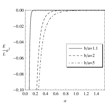
Here we have used the property that , and . The value of is obtained as the numerical solution of the differential equation. Using this technique we can obtain a numerical energy in about 1 cpu-second. The results of this calculation are found in figure 5.
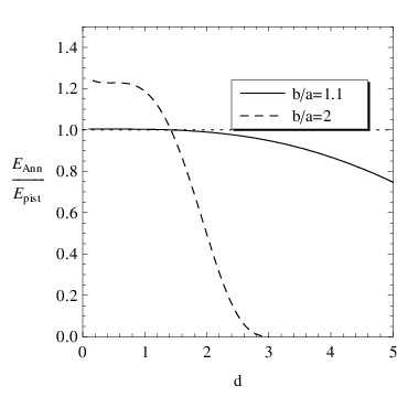
Again we would like to compare to known results, so figure 5 is a graph of the ratio of the energies of an annular piston, and a rectangular piston of similar dimension. The rectangular piston is constructed so it has the same finite width as the annular piston, and the separation distance is the mean distance between the annular plates,
| (16) |
The results make a certain amount of physical sense. The energy of the annular piston is greater than that of the rectangular piston for small separation because the inner edge of the annular piston is closer, and will contribute more to the energy. However as the annular piston gets further away, the other side of the piston will start to contribute and lower the overall energy. In addition we see that the energy for a small piston is much closer to that of the rectangular piston for small separations than for a larger piston, for vs. for . In both cases the value approached in the plateau in figure 5 is very close to the ratio of the energies of a flat plate to that of a tilted plate predicted by using the proximity force approximation.
Acknowledgments
This material is based upon work supported by the National Science Foundation under Grants Nos. PHY-0554926 (OU) and PHY-0757791 (BU) and by the US Department of Energy under Grants Nos. DE-FG02-04ER41305 and DE-FG02-04ER-46140 (both OU). We thank Simen Ellingsen, Iver Brevik, Prachi Parashar, Nima Pourtolami, and Elom Abalo for collaboration. Part of the work was done while KK enjoyed the hospitality and partial support of the Department of Physics and Astronomy of the University of Oklahoma. Thanks go in particular to Kimball Milton and his group who made this very pleasant and exciting visit possible.
References
- [1] H. B. G. Casimir, Proc. K. Ned. Akad. Wet. 60, 793 (1948).
- [2] M. Bordag, U. Mohideen and V. M. Mostepanenko, Phys. Rept. 353, 1 (2001).
- [3] K. A. Milton, J. Phys. A37, R209 (2004).
- [4] K. A. Milton, The Casimir effect: Physical manifestations of zero-point energy (World Scientific, River Edge, USA, 2001).
- [5] M. Bordag, G. L. Klimchitskaya, U. Mohideen and V. M. Mostepanenko, Advances in the Casimir Effect (Oxford University Press, New York, 2009).
- [6] M. J. Renne, Physica 56, 125 (1971).
- [7] T. Emig, Europhys. Lett. 62, 466 (2003).
- [8] A. Bulgac, P. Magierski and A. Wirzba, Phys. Rev. D73, 025007 (2006).
- [9] T. Emig, R. L. Jaffe, M. Kardar and A. Scardicchio, Phys. Rev. Lett. 96, 080403 (2006).
- [10] O. Kenneth and I. Klich, Phys. Rev. B 78, 014103 (2008).
- [11] P. M. Morse and H. Feshbach, Methods of Theoretical Physics: Part I (McGraw-Hill, 1953).
- [12] J. S. Dowker and G. Kennedy, J. Phys. A11, 895 (1978).
- [13] D. Deutsch and P. Candelas, Phys. Rev. D20, 3063 (1979).
- [14] H. Razmi and S. M. Modarresi, Int. J. Theor. Phys. 44, 229 (2005).
- [15] V. V. Nesterenko, G. Lambiase and G. Scarpetta, Annals Phys. 298, 403 (2002).
- [16] V. V. Nesterenko, I. G. Pirozhenko and J. Dittrich, Class. Quant. Grav. 20, 431 (2003).
- [17] A. A. Saharian and A. S. Tarloyan, J. Phys. A38, 8763 (2005).
- [18] A. A. Saharian and A. S. Tarloyan, Annals Phys. 323, 1588 (2008).
- [19] I. Brevik, S. A. Ellingsen and K. A. Milton, Phys. Rev. E 79, 041120 (2009).
- [20] S. A. Ellingsen, I. Brevik and K. A. Milton, Phys. Rev. E 80, 021125 (2009).
- [21] K. A. Milton, J. Wagner and K. Kirsten, Phys. Rev. D in press, arXiv:0911.2688.
- [22] T. M. Dunster, SIAM J. Math. Anal. 21, 995 (1990).
- [23] F. W. J. Olver, Asymptotics and Special Functions (Academic Press, New York, 1974).