The complete set of solutions of the geodesic equations in the space-time of a Schwarzschild black hole pierced by a cosmic string
Abstract
We study the geodesic equations in the space-time of a Schwarzschild black hole pierced by an infinitely thin cosmic string and give the complete set of analytical solutions of these equations for massive and massless particles, respectively. The solutions of the geodesic equations can be classified according to the particle’s energy and angular momentum, the ratio between the component of the angular momentum aligned with the axis of the string and the total angular momentum, the deficit angle of the space-time and as well the horizon radius (or mass) of the black hole. For bound orbits of massive test particles we calculate the perihelion shift, we discuss light deflection and comment on the Newtonian limit.
pacs
04.20.Jb, 02.30.HqI Introduction
The motion of test particles (both massive and massless) provides the only experimentally feasible way to study the gravitational fields of objects such as black holes. Predictions about observable effects (light deflection, gravitational time–delay, the perihelion shift and the Lense-Thirring effect) can be made and compared with observations. Geodesics in black hole space-times in 4 dimensional Schwarzschild space–time [1] and Kerr and Kerr–Newman space–time [2] have been discussed extensively. This has been extended to the cases of Schwarzschild–de–Sitter space-times [3] as well as to spherically symmetric higher dimensional space–times [4]. Recently also the general solution to the geodesic equation in 4 dimensional Kerr–de–Sitter [5] and even general Plebanski–Demianski space–times without acceleration has been found [6].
Cosmic strings have gained a lot of renewed interest over the past years due to their possible connection to string theory [7]. These are topological defects [8] that could have formed in one of the numerous phase transitions in the early universe due to the Kibble mechanism. Inflationary models resulting from string theory (e.g. brane inflation) predict the formation of cosmic string networks at the end of inflation [9].
Different space-times containing cosmic strings have been discussed in the past. This study has mainly been motivated by the pioneering work of Bach and Weyl [10] describing a pair of black holes held apart by an infinitely thin strut. This solution has later been reinterpreted in terms of cosmic strings describing a pair of black holes held apart by two cosmic strings extending to infinity in opposite direction. Consequently, a cosmic string piercing a Schwarzschild black hole has also been discussed, both in the thin string limit [11] – where an analytic solution can be given – as well as using the full U(1) Abelian-Higgs model [12, 13], where only numerical solutions are available. In the latter case, these solutions have been interpreted to represent black hole solutions with long range “hair” and are thus counterexamples to the No hair conjecture which states that black holes are uniquely characterized by their mass, charge and angular momentum. Interestingly, the solution found in [11] is a Schwarzschild solution which however differs from the standard spherically symmetric case by the replacement of the angular variable by , where the parameter is related to the deficit angle by . In this sense, the space-time is thus not uniquely determined by the mass, but is described by the mass and deficit angle parameter .
Schwarzschild black holes pierced by cosmic strings could have formed in phase transitions in the early universe. One possibility would be that the Coulomb field of a charged static, spherically symmetric black hole becomes confined within a flux tube during such a phase transition. Interestingly, this space–time has also been used to describe the exterior space–time of the sun taking into account departures from perfect spherical symmetry [14].
In order to understand details of gravitational fields of massive objects and to be able to predict observational consequences, it is important to understand how test particles move in these space-times.
Geodesics in the space–time of a Schwarzschild black hole pierced by a straight cosmic string have first been investigated in [15]. Spherical geodesics, i.e. geodesics in 3 spatial dimensions with constant radius as well as perturbations about spherical orbits in this space–time have been discussed in [16] and it has been observed that the angular momentum precesses around the symmetry axis of the cosmic string. The geodesics have also been discussed in [17] using the Hamilton-Jacobi formalism. However, neither [16] nor [17] provide a systematic study of all possible geodesics. The crucial point about the solutions of the geodesic equations is that elliptic integrals have to be solved which was neither attempted in [16] nor [17].
The aim of this paper is to determine the complete set of analytic solutions of the geodesic equations in the space–time of a Schwarzschild black hole pierced by a cosmic string and to derive analytical expressions for observable effects which can be used for astrophysical searches for such cosmic strings.
Our paper is organized as follows: in Section II, we give the geodesic equations and discuss the effective potential. In Section III, we classify the solutions and give examples for each class. In particularly we discuss the effect of the conical deficit on the geodesics. Section IV contains a short discussion about the Newtonian limit, while we conclude in Section V.
II The geodesic equations
We consider the geodesic equation
| (1) |
where denotes the Christoffel symbol given by
| (2) |
and is an affine parameter such that for time–like geodesics corresponds to proper time. The explicit form of the metric that we are studying in this paper is the metric of a Schwarzschild black hole pierced by a cosmic string [11] :
| (3) |
This metric describes a spherically symmetric static space-time with a conical deficit angle given by and an event horizon at the Schwarzschild radius . The deficit angle is directly proportional to the energy per unit length , which itself is equal to the tension of the string: . In addition we have , where is Newton’s constant. Note that is a parameter that is related to the physical mass of the black hole by [16] and can hence only be interpreted as the mass of the black hole if . is observable through the measurement of the event horizon radius by .
The Lagrangian for a point particle in the space–time (3) reads :
| (4) | |||||
where for massless particles and for massive particles, respectively.
The constants of motion are the energy and the component of the angular momentum of the particle that is aligned with the axis of the string (here the -axis) [16] :
| (5) | |||||
| (6) |
In addition
| (7) |
Here is the angular momentum vector, where
| (8) |
and
| (9) |
The modulus of the angular momentum is always conserved, however the direction of the angular momentum is only conserved for , i.e. in the “pure” Schwarzschild case.
Note that if we had used the Hamilton-Jacobi formalism here, the integration constant appearing in the separation of the equations –the so-called Carter constant– would have been equal to .
From variation of (4) and using the constants of motion, we obtain the geodesic equations :
| (10) | |||||
| (11) | |||||
| (12) | |||||
| (13) |
where here and in the following the dot denotes the derivative with respect to the affine parameter .
II.1 Effective potentials
II.2 and motion
In the following, we will be mainly interested in the radial motion, i.e. we will solve the geodesic equations for and . In order to do that we first have to eliminate the angular variable from (13). By dividing (12) by (13) we find [16]:
| (17) |
where =. This can be solved to give [16]:
| (18) |
Using (18), (11), (13) and (12) we find:
| (19) |
and
| (20) |
Orbits with are exactly the same as in the Schwarzschild case ), while for orbits with the presence of the deficit angle influences the shape of the orbits significantly. The orbits are in general non-planar (except for the case ) and lie in a plane that has as its normal. Since is not conserved, this plane precesses [16].
In [16], the simplest case of non-planar orbits, namely spherical orbits and perturbations around spherical orbits have been discussed. Here, we want to give the complete set of possible orbits in this space–time and discuss all related observables.
II.3 Classification of solutions
Using the new variable and introducing
| (21) |
we find from (19) and (20) using (18):
| (22) |
| (23) |
where the third order polynomial is given by
| (24) |
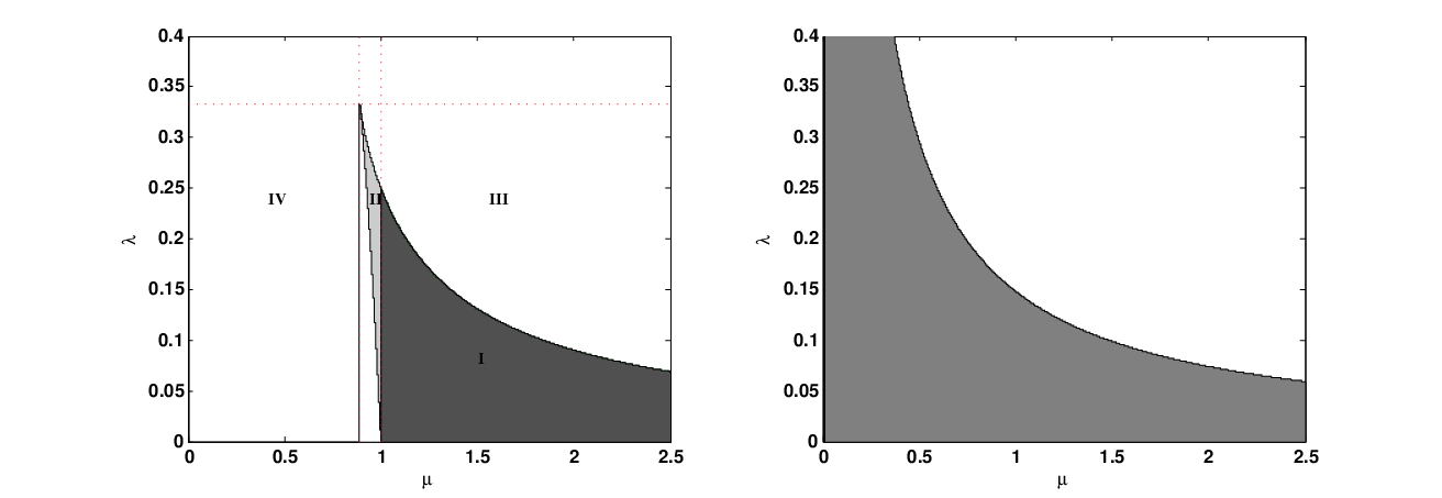
This is exactly the polynomial that appears in the case of the Schwarzschild solution and the classification of solutions is analogue. The main difference to the “pure” Schwarzschild case is that we have non-trivial integrals on the rhs of (22), (23). For a given and , the solutions can hence be classified according to the choice of and . Obviously, there are only solutions for . Hence, we can classify solutions according to the zeros of the characteristic polynomial and integrate (22), (23) for those for which . Note that in addition we can only integrate for such that . Depending on the sign of the discriminant of which is given by , the polynomial has either three real zeros , one real zero () or up to two real zeros for which we will denote by , and where in the following. This is illustrated in Fig.1 (left) for massive test particles (), where the shaded regions I and II correspond to positive , the boundary of the shaded region corresponds to and the unshaded regions III and IV correspond to negative . Note that only if and . We also give the corresponding plot for massless test particles () in Fig.1 (right). The shaded region corresponds to , the unshaded region to and the full boundary of the shaded region to . Note that () for () and that for or .
Comparing with (14), corresponds to the case for which , i.e. the total “energy” of the particle is smaller than the maximum and larger than the minimum of the effective potential . For then or , while for , or .
III Solutions of the geodesic equations
We can integrate (22)
| (25) |
and (23)
| (26) |
such that the general solutions for the radial motion in dependence on the angular variables read
| (27) |
where is the Weierstrass elliptic function and and are the functions appearing in (25) and (26), respectively. Our choice of depends on whether the orbit has finite maximal radius or whether it extends to infinity. For orbits with a finite maximal radius, we find it convenient to choose such that
| (28) |
while for orbits that extend to infinity we choose such that
| (29) |
In addition we choose for all cases such that from here on
| (30) |
The constant in (27) is given by . For we can always choose . For we choose for , for , for and for . Here
| (31) |
where denotes the complete elliptic integral of the first kind and is the modulus of the elliptic integral with
| (32) |
Moreover we have = . For , and there are various replacements of the Weierstrass function by real valued Jacobi elliptic functions [18].
In the following, we will discuss different type of orbits, which we denote as follows :
- 1.
Bound orbit : an orbit for which varies between two finite values.
- 2.
Spherical orbit : a special bound orbit for which is constant.
- 3.
Bound terminating orbit : a bound orbit that ends at the singularity .
- 4.
Unbound terminating orbit : an orbit for which varies between and infinity.
- 5.
Escape orbit : the orbit comes from infinity, approaches a finite and goes again to .
III.1 Geodesics for and
This case corresponds to the choice and (region I in the --plot). The effective potential and the corresponding characteristic polynomial are shown in Fig.2. The line intersects the effective potential twice. The polynomial has in fact three real zeros , , . However, for we have and in addition . We are hence allowed to integrate from to , which corresponds to integration from to and from to which corresponds to integration from to .
III.1.1 Escape orbit and light deflection
The range of allowed values for is indicated by the red horizontal line in Fig.2 and is .

The plots of escape orbits of a massive test particle and a massless test particle are given in Fig.3 and Fig.4, respectively. Obviously, for close to one, test particles get simply deflected. However, if is significantly smaller than one, particles will approach the minimal radius , then whirl the black hole and finally move off to infinity again. This is particularly important for the deflection of light.


In order to see the effect of on the deflection of light () we set (i.e. we choose ) and select the initial point at . The requirement imposes a bound on which reads:
| (33) |
Therefore the deflection angle is given by:
| (34) |
The term in the square bracket of (34) is the expression of for the “pure” Schwarzschild case, i.e. and the second term takes care of the fact that the space–time has a conical deficit.
Using the parametrized Post-Newtonian (PPN) formalism [20], which describes deviations from standard General Relativity, the angle of light deflection can be given by assuming that the parameter is equal to unity for General Relativity. denotes the General Relativity value assuming the exterior space-time of the massive body to be given by the Schwarzschild solution. Different experimental tests [21, 22, 23] have given a value of , hence . If we now assume that the deviations of from the Schwarzschild value are not due to a modification of General Relativity, but due to the presence of a cosmic string, we can approximate the energy per unit length of the cosmic string. Reinstalling factors of we then find which for the deficit angle gives . This transfers to a bound on the energy per unit length given by : .
III.1.2 Bound terminating orbit
The range of allowed values is indicated in Fig.2 and is . We don’t discuss this case in detail here, because it is qualitatively similar to the case with and (see discussion below).
III.2 Geodesics for and
This case corresponds to the choice and (region II in the --plot). The effective potential and the corresponding characteristic polynomial are shown in Fig. 5. The line intersects the effective potential three times at , and . These intersection points correspond to the zeros of the characteristic polynomial, which we denote by , and . Apparently, we are allowed to integrate between and , which corresponds to integration from to , and from to , which corresponds to integration from to .

III.2.1 Bound terminating orbit
The range of allowed values is indicated by the yellow line in Fig.5 and is .
A plot of a bound terminating orbit for a massive test particle is given in Fig. 6. We emphasize on the deformation of the orbits when changing the deficit parameter . While for , the orbit is still nearly planar, this changes with the decrease of , i.e. the increase of the deficit angle. While the orbit looks heart-shaped for , the increase of the deficit angle leads to a pretzel-like structure.


III.2.2 Bound orbit and perihelion shift
The range of allowed -values is indicated by the red line in Fig.5 and is .


A bound orbit of a massive test particle is given in Fig. 7 for different choices of . For close to one, the orbit corresponds to a standard closed orbit, while decreasing leads to the appearance of additional loops in the orbit (see the cases and ). This is important in order to understand the perihelion shift of test particles orbiting a massive body that is pierced by a cosmic string.
For bound orbits the perihelion shift depends on the deficit parameter . This effect has been calculated approximately in [14]. Here, we will give the exact analytic formula for the perihelion shift. We choose in order to study planar orbits with . We then have for the motion in the plane:
| (35) |
When the test particle moves from we find for the change in :
| (36) |
such that the perihelion shift reads
| (37) |
In Fig.8, we plot the value of in dependence on for , , and . Obviously, the perihelion shift can become quite large due to the conical nature of the space-time. Perihelion shifts in the solar system are quite small and the level of agreement of the measured value with that predicted by assuming the gravitational field of the sun to be described by the Schwarzschild solution can be used to give an upper bound on the energy density per unit length of a cosmic string present in the solar system. However, a large perihelion shift of per orbit has been observed in a massive binary black hole system [19]. Note that if we would do a similar approximation as that done in [14], we would find
| (38) |
where denotes the perihelion shift in the Schwarzschild case . Within the PPN formalism [20], the perihelion shift can be written as assuming that the parameters and are equal to unity for General Relativity and that the quadrupole moment of the sun vanishes. Different experimental tests [21, 22, 23] have given , hence .
If we now assume that the deviations of from the Schwarzschild value are not due to a modification of General Relativity, but due to the presence of a cosmic string, we can approximate the energy per unit length of the cosmic string. Again reinstalling factors of we find which for the deficit angle gives . This transfers to a bound on the energy per unit length which is given by : .

III.3 Geodesics for and
This case corresponds to the choice (region III in the --plot). The effective potential and the corresponding characteristic polynomial are shown in Fig. 9. The line does not intersect the effective potential . The polynomial has a single real zero at , however . We are allowed to integrate between and , which corresponds to integration from to .

III.3.1 Escape orbit
The range of allowed values is indicated by the red horizontal line in Fig.9 and corresponds to . The plot of an escape orbit in this case is shown in Fig.10. The particle comes in from infinity and – after a few loops – ends in .

III.4 Geodesics for and
This case corresponds to the choice (region IV in the --plot). The effective potential and the corresponding characteristic polynomial are shown in Fig. 11. The line intersects the effective potential only once at . This intersection point corresponds to the single real zero of the characteristic polynomial, which we denote by . Apparently, we are allowed to integrate between and , which corresponds to integration from to .
III.4.1 Bound terminating orbits

The range of allowed values is indicated by the red line in Fig.11 and is .

The example of a bound terminating orbit for a massive test particle for is given in Fig.12.
III.5 Geodesics for and
This case corresponds to the choice . The effective potential and the corresponding characteristic polynomial are shown in Fig. 13. The line intersects the effective potential only once at , i.e. at the maximum of the effective potential. This intersection point corresponds to a double zero of the characteristic polynomial, which we denote by . Apparently, we are allowed to integrate between and , which corresponds to integration from to and from to , which corresponds to integration from to .
Note that the spherical orbit with corresponds to the unstable spherical orbit discussed in [16].

III.5.1 Unbound terminating orbit
The range of allowed values is indicated by the yellow line in (13) and is .
An example of an unbound terminating orbit is given in Fig.14 for . The test particle comes from infinity and approaches an unstable spherical orbit with .
III.5.2 Bound terminating orbit
In this particular case the effective potential has its maximum at the maximal radius of the orbit. The range of allowed values is indicated by the red line in (13) and is .
An example of a bound terminating orbit is shown in Fig.15 for . The particle starts at and approaches the unstable spherical orbit at .


III.6 Geodesics for and
This case corresponds to the choice . The effective potential and the corresponding characteristic polynomial are shown in Fig. 16. The line intersects the effective potential at and at . These intersection points correspond to a double zero and a simple zero at . We are only allowed to integrate between and which corresponds to integration between and as well as between and which corresponds to integration between and .

III.6.1 Bound orbit
The range of allowed values is indicated in Fig.16 by the horizontal yellow line and is .
An example of a bound orbit is given in Fig.17 for . This is an example of a so-called homoclinic orbit. Homoclinic orbits are orbits that approach unstable circular orbits and have been discussed extensively in the context of gravitational wave production in binary system. There they play the role of a transition between the late inspiral and the final plunge [24].
III.6.2 Bound terminating orbit
In this particular case the effective potential has its maximum at the maximal radius of the orbit. An example of a bound terminating orbit is given in Fig.18.


III.7 Geodesics for and
This case corresponds to the choice . The effective potential and the corresponding characteristic polynomial are shown in Fig. 19. The line intersects the effective potential at . This corresponds to . We are allowed to integrate from to , which corresponds to integration from to .

III.7.1 Bound terminating orbit
III.7.2 Spherical orbit
For we have a spherical orbit. These spherical orbits have already been discussed in [16]. An example of a spherical orbit is given in Fig.21 for .


III.8 Geodesics for and
The effective potential and the corresponding characteristic polynomial are shown in Fig. 22. The line intersects the effective potential at and at the minimum of the effective potential at . These intersection points corresponds to a simple zero and a double zero at . We are only allowed to integrate between and , which corresponds to integration from to .

III.8.1 Bound terminating orbit
An example of a bound terminating orbit is shown in Fig.23.
III.8.2 Spherical orbit
Choosing we find a spherical orbit with radius . In this case, the spherical orbit is a stable spherical orbit. The qualitative plot is similar to the plot given in Fig.21.

IV Newtonian limit
Assuming the gravitational field to be weak and the test particles to move slowly, we can give the Newtonian limit of our equations. This reads [26]:
| (39) |
where we assume with very small and to be the Minkowski metric. Proceeding as in classical mechanics, we find the Virial theorem
| (40) |
where denotes the temporal average and is the kinetic energy. Hence, the Virial theorem doesn’t change for as compared to the Newtonian limit of the standard Schwarzschild case . However, note that the kinetic energy has a -dependence since
| (41) |
Since the average of the potential energy does not depend on and the Virial theorem holds for all this means that when the angular velocity increases. We have – in fact – seen this effect when studying the perihelion shift of planets. For the same interval of eigentime, the planet moves further in a space-time with as compared to in a space-time with .
In addition, it is easy to show that Kepler’s third law , where is the period of the orbit and the semimajor axis also doesn’t change. This is easiest to see when considering circular and planar orbits with , i.e. . For these, we let and substitute from into (see (11) and (12) ). After separation the two sides can be integrated to give the period of the orbit. The relation will contain a dependence on . However, note that the integration in is from to such that the cancels and and are independent of .
V Conclusions and Outlook
In this paper, we have constructed the complete set of geodesics in the space-time
of a Schwarzschild black hole pierced by a cosmic string.
We have classified the geodesics according to their energy, angular momentum aligned with the axis of the string , the ratio between total angular momentum and , the horizon
radius of the black hole and the deficit angle (or energy per unit length of the string).
We found that the change of the deficit angle doesn’t effect the motion, but that the motion changes significantly. Moreover, the motion
of the particles is in general not planar.
We found a bound of the energy per unit length of the string comparing our results
with experimental tests of General Relativity. From perihelion shift and light deflection
we found and , respectively.
The existence of cosmic strings may also influence the creation of gravitational waves since for inspirals and
flybys the deficit angle modifies the angular velocity and, thus, the temporal change of the effective quadrupole responsible for the emitted gravitational wave.
The results obtained in this paper can be generalized to rotating black holes, i.e.
to the space-time of a Kerr black hole pierced by a cosmic string. They can further be generalized to
a Schwarzschild–de Sitter black hole pierced by a cosmic string. For treating such orbits one has to
apply hyperelliptic integration developed in [3]. We expect the same enlarged variety
of orbits as we encountered in Schwarzschild–de Sitter space–time as compared to Schwarzschild space–time.
Acknowledgements
We thank the DFG and Jacobs University Bremen for financial support. We also thank A. Aliev for bringing
reference [15] to our attention.
References
- [1] Y. Hagihara, Theory of relativistic trajectories in a gravitational field of Schwarzschild, Japan. J. Astron. Geophys. 8, 67 (1931).
- [2] S.Chandrasekhar, The Mathematical Theory of black holes, Oxford University Press (1998).
- [3] E. Hackmann and C. Lämmerzahl, Phys. Rev. D 78 024035 (2008); Phys. Rev. Lett. 100, 171101 (2008).
- [4] E. Hackmann, V. Kagramanova, J. Kunz and C. Lämmerzahl, Phys. Rev. D 78 124018 (2008); [Erratum-ibid. 79 (2009) 029901]
- [5] E. Hackmann, V. Kagramanova, J. Kunz and C. Lämmerzahl, Analytic solutions of the geodesic equation in Kerr–(anti-)de Sitter space–times, Phys. Rev. D, to appear; E. Hackmann, C. Lämmerzahl, and A. Macias, Complete classification of geodesic motion in fast Kerr and Kerr–(anti-)de Sitter space–times, In:New trends in statistical physics: Festschrift in honour of Leopoldo Garcia-Colin’s 80th birthday (World Scientific, Singapore 2010), to appear.
- [6] E. Hackmann, V. Kagramanova, J. Kunz and C. Lämmerzahl, Europhys. Lett. 88, 30008 (2009).
- [7] see e.g. J. Polchinski, Introduction to cosmic F- and D-strings, hep-th/0412244 and reference therein.
- [8] A. Vilenkin and P. Shellard, Cosmic strings and other topological defects, Cambridge University Press (1994).
- [9] M. Majumdar and A. Davis, JHEP 03, 056 (2002); S. Sarangi and S. Tye, Phys. Lett.B 536, 185 (2002).
- [10] R. Bach and H. Weyl, Math. Zeit. 13, 134 (1922).
- [11] M. Aryal, L. Ford and A. Vilenkin, Phys. Rev. D 34, 2263 (1986)
- [12] F. Dowker, R. Gregory and J. Traschen, Phys. Rev. D 45, 2762 (1992).
- [13] A. Achucarro, R. Gregory and K. Kuijken, Phys. Rev. D 52, 5729 (1995).
- [14] W. Freire, V. Bezerra and J. Lima, Gen. Rel. Grav. 33 1407 (2001).
- [15] A. Aliev and D. Gal’tsov, Piz’ma Astron. Zh. 14, 116 (1988); translated in Sov. Astron. Lett. 14, 48 (1988).
- [16] D. Gal’tsov and E. Masar, Class. Quantum Grav. 6, 1313 (1989).
- [17] S. Chakraborty and L. Biswas, Class. Quantum Grav. 13, 2153 (1996).
- [18] M. Abramowitz, I. A. Stegun, 1972. Handbook of Mathematical Functions with Formulas, Graphs, and Mathematical Tables, 9th printing. New York: Dover, pp. 627-671.
- [19] M. J. Valtonen et. al, Nature 452, 851 (2008).
- [20] see e.g. C. Will, Theory and Experiment in Gravitational physics, Cambridge University Press (1993).
- [21] for a summary of recent results see e.g. S. Turyshev, Ann. Rev. Nucl. Part.Sci.58, 207 (2008)
- [22] J. Williams, S. Turyshev and D. Boggs, Phys. Rev. Lett. 93, 261101 (2004).
- [23] B. Bertotti, L. Iess and P. Tortora, Nature 425, 374 (2003).
- [24] J. Levin, R. O’Reilly and E. Copeland, (Sussex U.), Phys. Rev. D 62 024023 (2000).
- [25] M.G. Germano, V.B. Bezerra, E.R. Bezerra de Mello (1997), Class. Quantum Grav 13 2663 (1997)
- [26] see e.g. S. Carroll, Spacetime and Geometry: An Introduction to General Relativity, Benjamin Cummings (2003).