Consider a simple but typical experimental situation in which we have $n$ measurements $m_{i}$ of a single theoretical quantity $t$, with experimental uncertainties given by a covariance matrix $({\rm cov})_{ij}$: typically this takes the form

$$({\rm cov})_{ij}=\delta_{ij}\sigma_{i}^{2}+\sum_{k=1}^{n}\bar{\sigma}_{ik}\bar{\sigma}_{kj},$$

(1)

where the $\sigma_{i}$ are uncorrelated uncertainties (typically obtained as the sum in quadrature of statistical and uncorrelated systematic uncertainties) and $\bar{\sigma}_{ik}$ are correlated (typically systematic) uncertainties. All experimental uncertainties are generally assumed to be Gaussian. Then the least squares estimate for $t$ is given by minimizing the $\chi^{2}$ function

$$\chi^{2}(t)=\sum_{i,j=1}^{n}(t-m_{i})({\rm cov}^{-1})_{ij}(t-m_{j}),$$

(2)

and thus by

$$t={{\sum_{i,j=1}^{n}({\rm cov}^{-1})_{ij}m_{j}}\over{\sum_{i,j=1}^{n}({\rm cov}^{-1})_{ij}}}.$$

(3)

The variance of $t$, $V_{tt}$ is found through

$$V_{tt}=\Big(\hbox{${{{1}\over{2}}}$}{{\partial^{2}\chi^{2}}\over{\partial t^{2}}}\Big)^{-1}={{1}\over{\sum_{i,j=1}^{n}({\rm cov}^{-1})_{ij}}}.$$

(4)

Of course when there are several quantities $t$ to be determined, the variances are given by the diagonal elements $V_{tt}$ of the matrix determined by inversion of the Hessian matrix of second derivatives of $\chi^{2}$: hence the name of the method. Here the simplest case of only one quantity $t$ will be sufficient to illustrate the points we wish to make. The situation is yet more complicated when fitting parton distribution functions: then, $t$ is actually some nontrivial but calculable function (such as a cross section or structure function) of the (many) fitted parameters which describe the shape of the underlying parton distribution functions which is being determined. Again this complication is irrelevant to the issues to be discussed here, so we will ignore it.

In the very simplest case in which the measurements $m_{i}$ have completely uncorrelated (e.g. purely statistical) uncertainties $\sigma_{i}$,

$$({\rm cov})_{ij}=({\rm cov}_{0})_{ij}=\sigma_{i}^{2}\delta_{ij},$$

(5)

so

$$\chi^{2}(t)=\sum_{i=1}^{n}{{(t-m_{i})^{2}}\over{\sigma_{i}^{2}}},$$

(6)

whence at the minimum $t=w$ and $V_{tt}=\Sigma^{2}$, where

$$w\equiv\Sigma^{2}\sum_{i=1}^{n}{{m_{i}}\over{\sigma_{i}^{2}}},$$

(7)

and $\Sigma^{2}$ is given by

$${{1}\over{\Sigma^{2}}}=\sum_{i=1}^{n}{{1}\over{\sigma_{i}^{2}}}.$$

(8)

Thus the theoretical quantity $t$ is given by the average value of the measurements $m_{i}$ weighted by the inverses of the variances $\sigma_{i}^{2}$, and the inverse of the variance of $t$ is likewise the average of the inverses of the variances $\sigma_{i}^{2}$.

When all the variances are equal, $\sigma_{i}=\sigma$, and $w=\bar{m}$, where

$$\bar{m}={{1}\over{n}}\sum_{i=1}^{n}m_{i},$$

(9)

i.e. the unweighted average of the measurements. In this limiting case, the determination Eq. (3) of $t$ is manifestly seen to be unbiased (and in particular it tends to the true value in the limit of large number of measurements): no measurement is preferred, and $\Sigma^{2}=\sigma^{2}/n$, so the variance is reduced by a factor of $1/n$, due to there being $n$ independent measurements of the same quantity. In what follows we will use the words “biased” and “unbiased” to describe estimates of the mean which pass or fail this simple test.

In the opposite extreme, if one of the variances, say $\sigma_{i}^{2}$, becomes very large compared to the others, the contribution of the measurement $m_{i}$ to $w$ and $\Sigma^{2}$ becomes very small, so this measurement decouples from the rest as it must. In what follows we shall use freedom from bias (as defined above) and decoupling as two criteria to assess the usefulness of a particular method of determining $t$ and its variance.¹¹ 1 Note that the terms “bias” and “decoupling” as used here are not quite the same as the technical definitions of consistency and bias used by statisticians, which distinguish more carefully between results obtained with finite size samples and those when the sample size becomes infinite.

A different way of determining a theoretical quantity from a set of measurements is to construct a Monte Carlo representation of the data. First, the $n$ data points are associated to $n$ random variables $M_{i}$, normally distributed around the averages $m_{i}$ according to the covariance matrix $({\rm cov})_{ij}$. Then, an ensemble $\{M_{i}\}$ of replicas of the data is constructed: these by construction satisfy

$$\langle M_{i}\rangle=m_{i},\qquad\langle M_{i}M_{j}\rangle=m_{i}m_{j}+({\rm cov})_{ij},$$

(10)

where $\langle\rangle$ denotes averaging over the set of replicas. Finally an ensemble $\{T\}$ of replicas of the theoretical quantity $t$ is determined from the data replicas $\{M_{i}\}$, by minimizing a suitable error function $E_{\mathrm{MC}}(T)$. The mean value and variance of $t$ (and indeed any other function of $t$) may then be found simply by averaging over the replicas:

$${\rm E}[t]=\langle T\rangle,\quad{\rm Var}[t]=\langle T^{2}\rangle-\langle T\rangle^{2}.$$

(11)

This method becomes advantageous when the determination of some function of $t$ is called for: once the ensemble of replicas $\{T\}$ has been found, error propagation to any function of $t$, no matter how complicated, may be performed by simply averaging over replicas. This is especially useful in situations in which $t$ is multidimensional, or a nontrivial function of some underlying theoretical quantity (such as a PDF).

Clearly, the features of the result obtained with this method depend on the choice of error function $E_{\mathrm{MC}}(T)$ which determines the the ensemble of replicas $\{T\}$ from the data replicas $\{M_{i}\}$. In the simple situation discussed in the previous section we may choose $E_{\mathrm{MC}}(T)=\chi^{2}(T)$, where the $\chi^{2}$ function is given by Eq. (2). Then

$$T={{\sum_{i,j=1}^{n}({\rm cov}^{-1})_{ij}M_{j}}\over{\sum_{i,j=1}^{n}({\rm cov}^{-1})_{ij}}},$$

(12)

so that, using Eq. (11),

$${\rm E}[t]={{\sum_{i,j=1}^{n}({\rm cov}^{-1})_{ij}m_{j}}\over{\sum_{i,j=1}^{n}({\rm cov}^{-1})_{ij}}},$$

(13)

while

	$\displaystyle{\rm Var}[t]$	$\displaystyle=$	$\displaystyle{{\sum_{i,j,k,l=1}^{n}({\rm cov}^{-1})_{ij}({\rm cov}^{-1})_{kl}(\langle M_{j}M_{l}\rangle-\langle M_{j}\rangle\langle M_{l}\rangle)}\over{\left(\sum_{i,j=1}^{n}({\rm cov}^{-1})_{ij}\right)^{2}}}$		(14)
		$\displaystyle=$	$\displaystyle{{1}\over{\sum_{i,j=1}^{n}({\rm cov}^{-1})_{ij}}},$

in agreement with Eq. (3) and Eq. (4) found using the Hessian method.

The two methods discussed in the previous two sections cover most situations of uncorrelated and correlated errors found in combining experimental data. However problems arise when data sets have overall multiplicative uncertainties, such as normalization uncertainties: this is due to biases arising from the rescaling of errors [10, 11, 9]. The effect of these biases in the naive application of the Hessian method can be very severe, as will be discussed in the following section. Here we consider normalization uncertainties in the Monte Carlo method, which is possibly more straightforward.

First consider the situation in which all the data come from a single experiment, with a single overall normalization uncertainty $s$, assumed to be Gaussian. In the Monte Carlo method the normalization uncertainty is taken into account by multiplying the data by a random factor $N$, which is normally distributed around 1 with variance $s$. Assuming $N$ to be uncorrelated with $M_{i}$

$$\langle N\rangle=1,\qquad\langle N^{2}\rangle=1+s^{2},\qquad\langle f(N)g(M_{i})\rangle=\langle f(N)\rangle\langle g(M_{i})\rangle.$$

(15)

When fitting to the replicas, the error function will depend on $NM_{i}$, but the weights of the different measurements will be unchanged, since an overall rescaling of the data should not affect the relative weight of the measurements in the fit. Thus we now take

$$E_{\rm MC}(T)=\sum_{i,j=1}^{n}(T-NM_{i})({\rm cov}^{-1})_{ij}(T-NM_{j})$$

(16)

where $({\rm cov})_{ij}$ is the same covariance matrix used when there was no normalization uncertainty. The result of the minimization of Eq. (16) is the same as Eq. (12), but with an overall factor of $N$

$$T=N{{\sum_{i,j=1}^{n}({\rm cov}^{-1})_{ij}M_{j}}\over{\sum_{i,j=1}^{n}({\rm cov}^{-1})_{ij}}},$$

(17)

so ${\rm E}[t]$ is the same as in Eq. (13), while now

	$\displaystyle{\rm Var}[t]$	$\displaystyle=$	$\displaystyle{{\sum_{i,j,k,l=1}^{n}({\rm cov}^{-1})_{ij}({\rm cov}^{-1})_{kl}(\langle N^{2}\rangle\langle M_{j}M_{l}\rangle-\langle N\rangle^{2}\langle M_{j}\rangle\langle M_{l}\rangle)}\over{\left(\sum_{i,j=1}^{n}({\rm cov}^{-1})_{ij}\right)^{2}}}$		(18)
		$\displaystyle=$	$\displaystyle{{1+s^{2}}\over{\sum_{i,j=1}^{n}({\rm cov}^{-1})_{ij}}}+s^{2}{\rm E}[t]^{2}.$

The first term on the right–hand side of Eq. (18) is the same as was found previously in Eq. (14), but with an extra factor of $1+s^{2}$, while the second term is the contribution to the variance from the normalization uncertainty. This is as expected: indeed, the variance of a product of random variables is

$${\rm Var}[NM]={\rm E}[N]^{2}{\rm Var}[M]+{\rm E}[M]^{2}{\rm Var}[N]+{\rm Var}[N]{\rm Var}[M],$$

(19)

where the last term is usually neglected because, being a product of two variances, it corresponds to a higher order moment of the probability distribution for $NM$.

For the simple case of uncorrelated statistical measurement errors Eq. (5),

$$E_{\rm MC}(T)=\sum_{i=1}^{n}{{(T-NM_{i})^{2}}\over{\sigma_{i}^{2}}},$$

(20)

whence

$$T=N\Sigma^{2}\sum_{i=1}^{n}{{M_{i}}\over{\sigma_{i}^{2}}},$$

(21)

so ${\rm E}[t]=w$, Eq. (7), while

$${\rm Var}[t]=\Sigma^{2}+s^{2}w^{2}+s^{2}\Sigma^{2}.$$

(22)

Clearly then this method gives correct unbiased results for the case of a single experiment with normalization uncertainty.

Let us now consider a slightly more complex situation, where each of the measurements $m_{i}$ comes from a different experiment, and also has an independent normalization uncertainty $s_{i}$. Here and henceforth when discussing this situation we will neglect possible correlations between these measurements with independent uncertainties, which are usually absent if the measurements are obtained from independent experiments; however, the inclusion of such correlations is straightforward and it does not affect our subsequent results. Following the same line of reasoning as above, we want to derive the fitted value for $t$ and its variance in the Monte Carlo approach. We thus introduce independent normally distributed random variables $N_{i}$ to represent the normalization uncertainties, each with mean one, variance $s_{i}^{2}$, and uncorrelated to each other and to the $M_{i}$:

$$\langle N_{i}\rangle=1,\qquad\langle N_{i}N_{j}\rangle=1+s_{i}^{2}\delta_{ij},\qquad\langle f(N_{i})g(M_{j})\rangle=\langle f(N_{i})\rangle\langle g(M_{j})\rangle.$$

(23)

The difficulty now is to choose an appropriate error function. The simplest choice would be

$$E_{\rm MC}(T)=\sum_{i=1}^{n}{{(T-N_{i}M_{i})^{2}}\over{\sigma_{i}^{2}}},$$

(24)

Minimizing with respect to $T$ and averaging over the replicas then gives ${\rm E}[t]=w$ as before, but

	$\displaystyle{\rm Var}[t]$	$\displaystyle=$	$\displaystyle\Sigma^{4}\sum_{i,j=1}^{n}(\langle N_{i}N_{j}\rangle\langle M_{i}M_{j}\rangle-\langle N_{i}\rangle\langle N_{j}\rangle\langle M_{i}\rangle\langle M_{j}\rangle)/\sigma_{i}^{2}\sigma_{j}^{2},$		(25)
		$\displaystyle=$	$\displaystyle\Sigma^{2}+\Sigma^{4}\sum_{i=1}^{n}s_{i}^{2}(m_{i}^{2}+\sigma_{i}^{2})/\sigma_{i}^{4}.$

When all the experiments have the same normalization uncertainty, $s_{i}=s$, these results are not so unreasonable: ${\rm E}[t]=w$, while

$${\rm Var}[t]=(1+s^{2})\Sigma^{2}+s^{2}\Sigma^{4}\sum_{i=1}^{n}{{m_{i}^{2}}\over{\sigma_{i}^{4}}}\,.$$

(26)

However Eq. (24) is clearly incorrect in general because differences in the normalization uncertainties $s_{i}$ are not taken account of in the weighting of the different measurements. In particular if one of the experiments has a relatively large normalization uncertainty, it still contributes to the mean, but spoils the measurement by giving a very large contribution to the variance.

Therefore, results found using the Monte Carlo method with the error function Eq. (24) are unbiased when the normalization uncertainties are equal, but do not satisfy the criterion of decoupling. It follows that when we have more than one experiment, and in particular when we wish to include experiments with a large overall normalization uncertainty, we need to choose a better error function than Eq. (24), which incorporates differences in the normalization uncertainties $s_{i}$. We are thus led to consider error functions built using the full covariance matrix, including normalization uncertainties, and thus rather closer to the $\chi^{2}$-function.

Consider first a very simple model of a single experiment with only two data points. The covariance matrix Eq. (28) is then simply

$$({\rm cov}_{m})_{ij}=\left(\begin{array}[]{cc}\sigma_{1}^{2}+s^{2}m_{1}^{2}&s^{2}m_{1}m_{2}\cr s^{2}m_{1}m_{2}&\sigma_{2}^{2}+s^{2}m_{2}^{2}\cr\end{array}\right)$$

(30)

so the $\chi^{2}$ Eq. (27) is

$$\chi_{m}^{2}(t)={{(t-m_{1})^{2}(\sigma_{2}^{2}+m_{2}^{2}s^{2})+(t-m_{2})^{2}(\sigma_{1}^{2}+m_{1}^{2}s^{2})-2(t-m_{1})(t-m_{2})m_{1}m_{2}s^{2}}\over{\sigma_{1}^{2}\sigma_{2}^{2}+(m_{1}^{2}\sigma_{2}^{2}+m_{2}^{2}\sigma_{1}^{2})s^{2}}}\,.$$

(31)

Minimizing this $\chi^{2}$-function with respect to $t$ gives after a straightforward calculation the result

$$t={{m_{1}/\sigma_{1}^{2}+m_{2}/\sigma_{2}^{2}}\over{1/\sigma_{1}^{2}+1/\sigma_{2}^{2}+(m_{1}-m_{2})^{2}s^{2}/\sigma_{1}^{2}\sigma_{2}^{2}}}={{w}\over{1+(m_{1}-m_{2})^{2}s^{2}/\Sigma^{2}}},$$

(32)

where $w$ is the weighted mean Eq. (7) with $n=2$.

It follows that when $m_{1}\neq m_{2}$ and $s\neq 0$ the result for $t$ has a downward shift. That this shift is clearly a bias can be seen for instance by considering the simple case $\sigma_{1}=\sigma_{2}=\sigma$. Then Eq. (32) gives

$$t={{\bar{m}}\over{1+2r^{2}s^{2}\bar{m}^{2}/\sigma^{2}}}=\bar{m}(1-2r^{2}s^{2}\bar{m}^{2}/\sigma^{2}+O(r^{4})).$$

(33)

where we have defined

$$\bar{m}\equiv\hbox{${{{1}\over{2}}}$}(m_{1}+m_{2}),\qquad r\equiv{{m_{1}-m_{2}}\over{m_{1}+m_{2}}}.$$

(34)

Thus simply minimizing the $\chi^{2}$ derived from the correlated covariance matrix Eq. (28) leads to a central value which is shifted downwards: for a sufficiently large $s^{2}/\sigma^{2}$ one can get an average which is lower than either of the two values which are being averaged, so one must conclude that the result is biased.

This bias gets worse as the number of data points increases [11, 9, 12]. For $n$ data $m_{i}$, with statistical uncertainties $\sigma_{i}$, the covariance matrix given by Eq. (28) and Eq. (5) has inverse

$$({\rm cov}_{m}^{-1})_{ij}={{\delta_{ij}}\over{\sigma_{i}^{2}}}-{{m_{i}m_{j}}\over{\sigma_{i}^{2}\sigma_{j}^{2}}}{{s^{2}}\over{1+s^{2}m^{2}/\Sigma^{2}}}.$$

(35)

where

$$m^{2}\equiv\Sigma^{2}\sum_{i=1}^{n}{{m_{i}^{2}}\over{\sigma_{i}^{2}}}.$$

(36)

The $\chi^{2}$-function Eq. (27) is then minimized when

$$t={{\sum_{i,j=1}^{n}({\rm cov}_{m}^{-1})_{ij}m_{j}}\over{\sum_{i,j=1}^{n}({\rm cov}_{m}^{-1})_{ij}}}={{w}\over{1+r^{2}s^{2}w^{2}/\Sigma^{2}}}$$

(37)

where $w$ is defined in Eq. (7) while $r$ is defined through

$$m^{2}-w^{2}=\Sigma^{2}\sum_{i=1}^{n}{{(m_{i}-w)^{2}}\over{\sigma_{i}^{2}}}\equiv r^{2}w^{2}.$$

(38)

So again we have a downwards bias unless $s^{2}=0$ or all the measurements $m_{i}$ are equal. Note further that when the data are consistent and $n$ is large, $r^{2}$ is simply given by the variance $\Sigma^{2}$ of the measurements: $r^{2}w^{2}\simeq n\Sigma^{2}$. The bias is thus by a factor $1/(1+ns^{2})$, which will become arbitrarily large as the number of data points increases.

The origin of the bias is clear: smaller values of $m_{i}$ have a smaller normalization uncertainty $m_{i}s$, and are thus preferred in the fit. Several examples of situations where this leads to absurd results may be found in Ref. [9]. The variance of $t$ is afflicted by the same downward bias:

$$V_{tt}={{\Sigma^{2}+s^{2}w^{2}(1+r^{2})}\over{1+r^{2}s^{2}w^{2}/\Sigma^{2}}}.$$

(39)

We will henceforth refer to this as the “d’Agostini bias”, after Ref. [9, 11] where it was studied and explained.

In the second example with $n$ distinct experiments the d’Agostini bias is much milder. With the covariance matrix Eq. (29), the $\chi^{2}$-function is

$$\chi_{m}^{2}(t)=\sum_{i=1}^{n}{{(t-m_{i})^{2}}\over{\sigma_{i}^{2}+m_{i}^{2}s_{i}^{2}}}\,,$$

(40)

which is minimized when

$$t={{\sum_{i=1}^{n}{{m_{i}}\over{\sigma_{i}^{2}+s^{2}m_{i}^{2}}}}\over{\sum_{i=1}^{n}{{1}\over{\sigma_{i}^{2}+s^{2}m_{i}^{2}}}}}.$$

(41)

To exhibit the bias, consider again the case when all statistical uncertainties are equal, $\sigma_{i}=\sigma$: then on expanding in powers of

$$r^{2}\equiv{{1}\over{n}}\sum_{i=1}^{n}{{(m_{i}-\bar{m})^{2}}\over{\bar{m}^{2}}}={{1}\over{n}}\sum_{i=1}^{n}{{m_{i}^{2}-\bar{m}^{2}}\over{\bar{m}^{2}}},$$

(42)

with $\bar{m}$ given by Eq. (9) we find

$$t=\bar{m}\left(1-2r^{2}{{s^{2}\bar{m}^{2}}\over{\sigma^{2}+s^{2}\bar{m}^{2}}}+O(r^{4})\right).$$

(43)

The origin of the bias is the same as in Eqs. (33,37), and indeed for two data points the biases are approximately the same: however for $n$ independent experiments, the bias Eq. (43) is stable for large $n$. In this case the variance is given by (again expanding in $r$)

$$V_{tt}=\hbox{${{{1}\over{n}}}$}(\sigma^{2}+s^{2}\bar{m}^{2}(1+r^{2}))+O(r^{4}),$$

(44)

which is as expected, since $\bar{m}^{2}(1+r^{2})={{1}\over{n}}\sum_{i=1}^{n}m_{i}^{2}$.

We first consider a single experiment, with covariance matrix Eq. (5), but now with an overall normalization uncertainty with variance $s^{2}$. The value of $t$ is then obtained by minimizing the error function

$$E_{\rm Hess}(t,n)=\sum_{i=1}^{n}{{(t/n-m_{i})^{2}}\over{\sigma_{i}^{2}}}+{{(n-1)^{2}}\over{s^{2}}}\,.$$

(45)

where the last term is called the penalty term. The parameters $t$ and $n$ are then determined by minimizing this error function: minimizing with respect to $t$ gives $t=nw$, with $w$ as defined in Eq. (7), while minimization with respect to $n$ fixes $n=1$, so for the central values the result is the same as in the Monte Carlo approach.²² 2 Note that to obtain an unbiased result from this approach, the factor $n$ must rescale the theory, not the data: if instead of Eq. (45) we took $$E_{\rm Hess}=\sum_{i=1}^{n}{{(t-nm_{i})^{2}}\over{\sigma_{i}^{2}}}+{{(n-1)^{2}}\over{s^{2}}}\,.$$ we would get a result with a strong downward bias similar to that in Eq. (37) [11, 9].

In order to compute the error on the fitted quantity in this approach, we need to evaluate the Hessian matrix:

$$V^{-1}=\hbox{${{{1}\over{2}}}$}\begin{pmatrix}\hbox{${{{\partial^{2}\chi^{2}}\over{\partial t^{2}}}}$}&\hbox{${{{\partial^{2}\chi^{2}}\over{\partial t\partial n}}}$}\\ \hbox{${{{\partial^{2}\chi^{2}}\over{\partial n\partial t}}}$}&\hbox{${{{\partial^{2}\chi^{2}}\over{\partial n^{2}}}}$}\end{pmatrix}={{1}\over{\Sigma^{2}}}\begin{pmatrix}1&-t\\ -t&\Sigma^{2}/s^{2}+t^{2}\end{pmatrix}\,.$$

(46)

The covariance matrix is obtained by inverting $V^{-1}$. In this way one recovers

$$V_{tt}=\Sigma^{2}+s^{2}w^{2}\,.$$

(47)

This is the same result as Eq. (22) obtained with the Monte Carlo approach, apart from the cross-correlation term between the variances of the measurements and the variances of the normalization, akin to the last term in Eq. (19).

For the case of a single experiment, we have thus recovered within the Hessian approach the Monte Carlo result of Sect. 2.3: in this simple case the Hessian and Monte Carlo methods are (almost) equivalent. It is straightforward to generalize this equivalence to a general covariance matrix Eq. (1).

Let us now turn to the more complex situation where we have several data points from different experiments, and thus with independent normalizations, $n_{i}=1\pm s_{i}$. In this case, the Monte Carlo result Eq. (25) is unbiased (in the sense that it gives an unbiased average over the data when all uncertainties are equal), but it does not satisfy the requirement of decoupling. We will now show that the penalty trick leads to a result which does satisfy decoupling, but is biased when all uncertainties are equal.

Following the same line of reasoning as for the single experiment above, we set up the error function

$$E_{\rm Hess}(t,n_{i})=\sum_{i=1}^{n}{{(t/n_{i}-m_{i})^{2}}\over{\sigma_{i}^{2}}}+\sum_{i=1}^{n}{{(n_{i}-1)^{2}}\over{s_{i}^{2}}}\,,$$

(48)

where now we have a separate penalty term for each of the normalizations to be fitted. The minimum is obtained for

	$\displaystyle t$	$\displaystyle=$	$\displaystyle{{\sum_{i=1}^{n}{{m_{i}}\over{n_{i}\sigma_{i}^{2}}}}\over{\sum_{i=1}^{n}{{1}\over{n_{i}^{2}\sigma_{i}^{2}}}}},$		(49)
	$\displaystyle n_{i}$	$\displaystyle=$	$\displaystyle 1+{{s_{i}^{2}t}\over{n_{i}^{2}\sigma_{i}^{2}}}\left({{t}\over{n_{i}}}-m_{i}\right)\,.$		(50)

These $n+1$ equations are now complicated nonlinear relations which must be solved for $t$ and $n_{i}$. A general analytic solution is probably impossible, and it seems very likely that for a large number of experiments the number of solutions will grow rapidly, making it difficult to select the correct one. However it is possible to find solutions for certain special cases, which are sufficient to show that the approach is biased.

First we specialize to the case of only two experiments: to explore the bias we again assume that $\sigma_{1}=\sigma_{2}\equiv\sigma$ and $s_{1}=s_{2}=s$, as in Sect. 3.1. Adding and subtracting the two equations for $n_{1}$ and $n_{2}$, and substituting the equation for $t$, we find

$$n_{1}^{2}+n_{2}^{2}=n_{1}+n_{2}\,,\qquad n_{1}^{2}-n_{2}^{2}=-2\Delta n_{1}n_{2}\,,$$

(51)

where

$$\Delta={{s^{2}}\over{\sigma^{2}+m_{1}m_{2}s^{2}}}\hbox{${{{1}\over{2}}}$}(m_{1}^{2}-m_{2}^{2})\,.$$

(52)

Solving these for $n_{1}$ and $n_{2}$, and choosing the solution close to one (note that $\Delta$ will generally be rather small) gives

	$\displaystyle n_{i}$	$\displaystyle=$	$\displaystyle\hbox{${{{1}\over{2}}}$}\left(1+{{1\mp\Delta}\over{\sqrt{1+\Delta^{2}}}}\right),$		(53)
	$\displaystyle t$	$\displaystyle=$	$\displaystyle\bar{m}{{\hbox{${{{1}\over{2}}}$}(1+\sqrt{1+\Delta^{2}}+r\Delta)}\over{1+\Delta^{2}}},$		(54)

where $\bar{m}$ and $r$ are defined in Eq. (34).

The variance may now be computed as before by inversion of the three by three Hessian matrix. The result is not very enlightening, however it simplifies if we expand in powers of $r$: the Hessian method then gives

	$\displaystyle t$	$\displaystyle=$	$\displaystyle\bar{m}\Big(1+{{s^{2}\bar{m}^{2}(\sigma^{2}-2s^{2}\bar{m}^{2})}\over{(\sigma^{2}+s^{2}\bar{m}^{2})^{2}}}r^{2}+O(r^{4})\Big),$		(55)
	$\displaystyle V_{tt}$	$\displaystyle=$	$\displaystyle\hbox{${{{1}\over{2}}}$}\sigma^{2}+\hbox{${{{1}\over{2}}}$}s^{2}\bar{m}^{2}\Big(1+r^{2}-4{{(2\sigma^{2}+s^{2}\bar{m}^{2})^{2}}\over{(\sigma^{2}+s^{2}\bar{m}^{2})^{3}}}s^{2}\bar{m}^{2}r^{2}+O(r^{4})\Big)\,.$		(56)

Clearly, both the central value and variance Eqs. (55,56) are biased: the normalization uncertainties leads to data being weighed differently based on their central values, even when their normalization uncertainties are the same. It is not difficult to show from the structure of Eqs. (49,50) that the results Eqs. (55,56) remain true for any number of data points, i.e. for all $n\geq 2$, provided that $\bar{m}$ and $r$ are defined as in Eqs. (9,38), and an overall factor of $2/n$ is included in the variance.

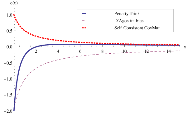
This bias is more subtle than the d’Agostini bias Eq. (43), in that it is caused by nonlinearities in the error function rather than by a consistent bias in the variances. It can thus have either sign, depending on the relative weight of statistical and normalization uncertainties: we can rewrite Eqs. (55-56) in the form

	$\displaystyle t$	$\displaystyle=$	$\displaystyle\bar{m}\big(1+c(\hbox{${{{\sigma^{2}}\over{s^{2}\bar{m}^{2}}}}$})r^{2}+O(r^{4})\big),$		(57)
	$\displaystyle V_{tt}$	$\displaystyle=$	$\displaystyle\hbox{${{{1}\over{n}}}$}\sigma^{2}+\hbox{${{{1}\over{n}}}$}s^{2}\bar{m}^{2}\big(1+r^{2}+v(\hbox{${{{\sigma^{2}}\over{s^{2}\bar{m}^{2}}}}$})r^{2}+O(r^{4})\big)\,,$		(58)

with the functions $c$ and $v$ given by

$$c(x)={{x-2}\over{(x+1)^{2}}},\qquad v(x)=-4{{(2x-1)^{2}}\over{(x+1)^{3}}}.$$

(59)

The unbiased results would correspond to $c=v=0$. The d’Agostini–biased results Eqs. (43-44) can also be cast in the form of Eq. (57-58), but now with $c(x)=-2/(x+1)$, $v(x)=0$ (since in this case the variance is unbiased at $O(r^{2})$).

The “bias” functions $c(x)$ and $v(x)$ for these two cases, as well as for a further biased case to be discussed below in Sect. 5, are compared in Fig. 1. Thanks to the penalty trick, the bias in the central value is generally less severe, but the variance is now also biased.

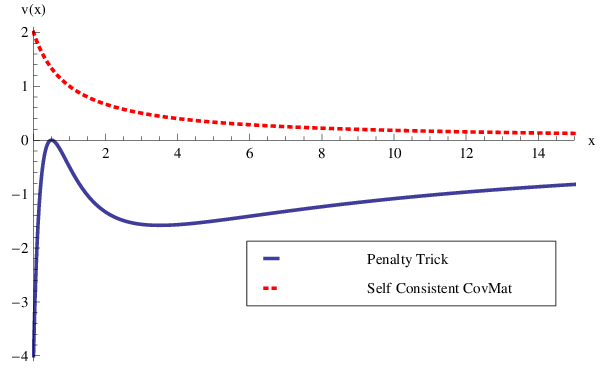
It is also interesting to explore decoupling in this approach. To do this we again consider two experiments, in the special case in which the normalization errors dominate, so $\sigma_{1}^{2},\sigma_{2}^{2}\ll s_{1}^{2}m_{1}^{2},s_{2}^{2}m_{2}^{2}$. Then Eqs.(49,50) can again be solved: $n_{i}=t/m_{i}$, with

$$t=m_{1}m_{2}{{m_{1}s_{1}^{2}+m_{2}s_{2}^{2}}\over{m_{1}^{2}s_{1}^{2}+m_{2}^{2}s_{2}^{2}}}.$$

(60)

The variance is now

$$V_{tt}=m_{1}^{2}m_{2}^{2}{{s_{1}^{2}s_{2}^{2}}\over{m_{1}^{2}s_{1}^{2}+m_{2}^{2}s_{2}^{2}}}.$$

(61)

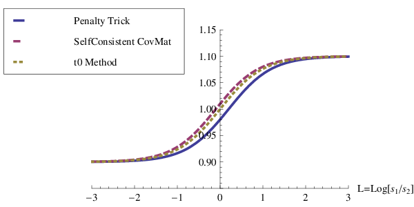
When $s_{1}\ll s_{2}$, we recover $t=m_{1}$ and $V_{tt}=m_{1}^{2}s_{1}^{2}$, as we should. However the result Eq. (60) looks rather strange: one would expect that in this limit the measurements $m_{1}$ and $m_{2}$ to be simply weighted by $1/s_{1}^{2}$ and $1/s_{2}^{2}$, in analogy to the weighting Eq. (7) in the single experiment case, and the variance to be a similar weighted average of $m_{1}^{2}$ and $m_{2}^{2}$ (see Eqs. (98–99) below). Instead the weighting is more complicated, reflecting the bias in this method for general $s_{1}\neq s_{2}$. Note for example that when $s_{1}=s_{2}$, $t=m_{1}m_{2}(m_{1}+m_{2})/(m_{1}^{2}+m_{2}^{2})\neq\hbox{${{{1}\over{2}}}$}(m_{1}+m_{2})$, and $V_{tt}=s^{2}m_{1}^{2}m_{2}^{2}/(m_{1}^{2}+m_{2}^{2})\neq\hbox{${{{1}\over{4}}}$}s^{2}(m_{1}^{2}+m_{2}^{2})$. The result Eq. (60) is shown in Fig. 2 for the special case $m_{1}=0.9$ and $m_{2}=1.1$. The bias is readily apparent in the asymmetry of the curve.

The generalization to $n$ independent experiments is straightforward in this limit: Eq. (60) becomes

$$t={{\sum_{i=1}^{n}{{1}\over{m_{i}s_{i}^{2}}}}\over{\sum_{i=1}^{n}{{1}\over{m_{i}^{2}s_{i}^{2}}}}},$$

(62)

so if $s_{i}=s$, when there should be no bias, we have instead $t=\sum_{i=1}^{n}m_{i}^{-1}/\sum_{i=1}^{n}m_{i}^{-2}\neq\bar{m}$ unless $m_{i}=m$.

With two measurements within a single experiment, we now have a covariance matrix

$$({\rm cov}_{t})_{ij}=\left(\begin{array}[]{cc}\sigma_{1}^{2}+s^{2}t^{2}&s^{2}t^{2}\cr s^{2}t^{2}&\sigma_{2}^{2}+s^{2}t^{2}\cr\end{array}\right)$$

(64)

so the $\chi^{2}$ is

$$\chi^{2}_{t}(t)={{(t-m_{1})^{2}(\sigma_{2}^{2}+t^{2}s^{2})+(t-m_{2})^{2}(\sigma_{1}^{2}+s^{2}t^{2})-2(t-m_{1})(t-m_{2})s^{2}t^{2}}\over{\sigma_{1}^{2}\sigma_{2}^{2}+(\sigma_{1}^{2}+\sigma_{2}^{2})s^{2}t^{2}}}\,.$$

(65)

It is easy to check that minimizing this $\chi^{2}$ with respect to $t$ gives again $t=w$, where $w$ is the weighted average Eq. (7). The variance $V_{tt}$ is now simply the inverse of the second derivative of the $\chi^{2}$ Eq. (31) at the minimum: a straightforward but tedious calculation then leads back to Eq. (47).

It is not difficult to show that everything works out for a general covariance matrix Eq. (63) for a single experiment with $n$ data:

	$\displaystyle\hbox{${{{1}\over{2}}}$}{{\partial\chi^{2}_{t}}\over{\partial t}}$	$\displaystyle=$	$\displaystyle\sum_{i,j=1}^{n}({\rm cov}_{t}^{-1})_{ij}(t-m_{j})+\hbox{${{{1}\over{2}}}$}\sum_{i,j=1}^{n}(t-m_{i})\left({{\partial{\rm cov}_{t}^{-1}}\over{\partial t}}\right)_{ij}(t-m_{j})$		(66)
		$\displaystyle=$	$\displaystyle\sum_{i,j=1}^{n}({\rm cov}_{t}^{-1})_{ij}(t-m_{j})-\hbox{${{{1}\over{2}}}$}\sum_{i,j,k,l=1}^{n}(t-m_{i})({\rm cov}_{t}^{-1})_{ik}\left({{\partial{\rm cov}_{t}}\over{\partial t}}\right)_{kl}({\rm cov}_{t}^{-1})_{lj}(t-m_{j})$
		$\displaystyle=$	$\displaystyle\sum_{i,j=1}^{n}({\rm cov}_{t}^{-1})_{ij}(t-m_{j})\Big[1-s^{2}t\sum_{k,l=1}^{n}({\rm cov}_{t}^{-1})_{lk}(t-m_{k})\Big],$

which vanishes when

$$t={{\sum_{i,j=1}^{n}({\rm cov}_{t}^{-1})_{ij}m_{j}}\over{\sum_{i,j=1}^{n}({\rm cov}_{t}^{-1})_{ij}}}\,.$$

(67)

The variance of $t$ is given by evaluating ${{\partial^{2}\chi_{t}^{2}}\over{\partial t^{2}}}$ at the minimum: this yields

$$V_{tt}={{1}\over{\sum_{i,j=1}^{n}({\rm cov}_{t}^{-1})_{ij}}}\,.$$

(68)

When

$$({\rm cov}_{t})_{ij}=\delta_{ij}\sigma^{2}_{i}+s^{2}t^{2}\ ,$$

(69)

the inverse is

$$({\rm cov}_{t}^{-1})_{ij}={{\delta_{ij}}\over{\sigma^{2}_{i}}}-{{s^{2}t^{2}}\over{\sigma_{i}^{2}\sigma_{j}^{2}}}{{\Sigma^{2}}\over{\Sigma^{2}+s^{2}t^{2}}}\ ,$$

(70)

where $\Sigma$ is as defined in Eq. (8). Thus Eq. (67) and Eq. (68) simplify to the familiar results $t=w$ Eq. (7) and $V_{tt}=\Sigma^{2}+s^{2}w^{2}$ Eq. (47).

Note however that since $\chi_{t}^{2}$ Eq. (31) is no longer quadratic in $t$, there is also a spurious solution: the term in square brackets in Eq. (66) vanishes when $t=\Sigma^{2}/ws^{2}$ which might be troublesome since it may lie close to the correct solution $t=w$ whenever $s^{2}w^{2}\sim\Sigma^{2}$.

Consider now the case of $n$ independent experiments. The covariance matrix is then

$$({\rm cov}_{t})_{ij}=(\sigma_{i}^{2}+s_{i}^{2}t^{2})\delta_{ij},$$

(71)

so the $\chi^{2}$ is

$$\chi^{2}_{t}(t)=\sum_{i=1}^{n}{{(t-m_{i})^{2}}\over{\sigma_{i}^{2}+s_{i}^{2}t^{2}}}\,.$$

(72)

The minimum of $\chi_{t}^{2}$ is found by solving the system of nonlinear equations

$$\sum_{i=1}^{n}{{(t-m_{i})(tm_{i}s_{i}^{2}+\sigma_{i}^{2})}\over{(t^{2}s_{i}^{2}+\sigma_{i}^{2})^{2}}}=0\,.$$

(73)

In general these equations will have $4n-2$ solutions, so for a large number of experiments finding the correct solution might be difficult.

References

- [1] M. Dittmar et al., arXiv:hep-ph/0511119. M. Dittmar et al., arXiv:0901.2504 [hep-ph].
- [2] S. Forte, L. Garrido, J. I. Latorre and A. Piccione, JHEP 0205 (2002) 062 [arXiv:hep-ph/0204232].
- [3] L. Del Debbio, S. Forte, J. I. Latorre, A. Piccione and J. Rojo [NNPDF Collaboration], JHEP 0503 (2005) 080 [arXiv:hep-ph/0501067].
- [4] L. Del Debbio, S. Forte, J. I. Latorre, A. Piccione and J. Rojo [NNPDF Collaboration], JHEP 0703 (2007) 039 [arXiv:hep-ph/0701127].
- [5] R. D. Ball et al. [NNPDF Collaboration], Nucl. Phys. B 809 (2009) 1 [Erratum-ibid. B 816 (2009) 293] [arXiv:0808.1231 [hep-ph]].
- [6] J. Rojo et al. [NNPDF Collaboration], arXiv:0811.2288 [hep-ph].
- [7] R. D. Ball et al. [The NNPDF Collaboration], Nucl. Phys. B 823, 195 (2009) [arXiv:0906.1958 [hep-ph]].
- [8] W. T. Giele, S. A. Keller and D. A. Kosower, arXiv:hep-ph/0104052.
- [9] G. D’Agostini, ”Bayesian reasoning in data analysis: A critical introduction”, World Scientific, 2003.
- [10] H.J. Behrend et al [CELLO Collaboration], Phys. Lett. B183 (1987) 400.
- [11] G. D’Agostini, Nucl. Instrum. Meth. A346 (1994) 306.
- [12] T. Takeuchi, Prog. Theor. Phys. Suppl. 123 (1996) 247.
- [13] F.D. Aaron et al, Eur. Phys. J. C63 (2009) 625; JHEP 1001 (2010) 109 [arXiv:0911.0884 [hep-ex]].
- [14] W.T. Eadie, D. Dryard, F.E. James, M. Roos and B. Sadoulet, “Statistical Methods in Experimental Physics”, North Holland (1971).
- [15] R. D. Ball et al. [The NNPDF Collaboration], [arXiv:1002.4407 [hep-ph]].
- [16] A. D. Martin, W. J. Stirling, R. S. Thorne and G. Watt, Eur. Phys. J. C 63, 189 (2009) [arXiv:0901.0002 [hep-ph]].
- [17] P. M. Nadolsky et al., Phys. Rev. D 78 (2008) 013004 [arXiv:0802.0007 [hep-ph]].
- [18] P. M. Nadolsky, private communication
- [19] L. Lyons, A.J. Martin and D.H. Saxon, Phys. Rev. D41 (1990) 982.