Transverse radiation force in a tailored optical fiber

Recent years have seen an increased interest in radiation forces in optics. Optical tweezers, atom traps, optical manipulation of soft materials such as interfaces between liquids - especially near the critical point where surface tension is small - are typical examples. This trend will in all probability continue in the time to come.

Our objective in the present Communication is to point towards the possibility - to our knowledge not so far contemplated in the literature - to create a tailored transverse optical force in a fiber transmitted by a laser beam. The beam may be pulsed, or it may be continuous. The clue of the principle is to introduce an accurate mechanical imbalance in the fiber, implying a slight asymmetry in the refractive index $n$. (In practice, such a deviation from axisymmetry may easily result inadvertently, during the mechanical drawing of the fiber.) If one side of the fiber is harder than the other, there may be a slight refractive index difference $\Delta n$ between the two sides, resulting in a transverse optical force. As fibers of micron scale cross sections are very light and bend easily, a sideways motion may easily occur. The effect, besides being of basic interest, may be of practical utility. We will describe the effect, making use of simple models for the fiber, and thereafter compare with a recent experiment which in our opinion has most likely already observed this effect.

The problem is to some extent related to the one-hundred years old Abraham-Minkowski debate on the correct electromagnetic energy-momentum tensor in dielectric media. From a physical point of view the key issue is that one is dealing with a nonclosed system, matter and field. Macroscopic of phenomenological electromagnetic theory implying the use of a permittivity $\varepsilon$ and permeability $\mu$ means that one is dealing with a complicated interaction system involving external fields, internal fields, and constituent molecules, by using only simple material parameters. The solution to the problem lies in extracting the energy-momentum form that leads to a theoretical description of observable effects in a clean and simple manner. For an overview of the Abraham-Minkowski debate, cf. e.g. [1]. There exist at present a great number of papers discussing the Abraham-Minkowski problem, for instance the recent Ref. [2] and the review [3].

Assume now for definiteness that the fiber is vertically hanging, and that a laser pulse is transmitted through it. The general expression for the electromagnetic force density in the medium, assumed hereafter nonmagnetic, is derived from a given stress tensor $\sigma_{ik}$ as $f_{i}=\partial_{k}\sigma_{ik}$. For the Abraham and Minkowski tensors this implies (c.f. Refs. [1, 4] for details)

Here ${\bf f}^{\mathrm{AM}}=-(\varepsilon_{0}/2)\tilde{E}^{2}{\bf\nabla}n^{2}$ is nonvanishing in any region where $n$ varies, especially in the surface regions. We use notation $\tilde{\mathbf{E}}(\mathbf{r},t)=\mathrm{Re}\{\mathbf{E}(x)e^{i(\omega t-\beta z)}\}$ and skip the exponential factor in the following (c.f. [5] Ch. 1.3, for notational details). As this force is common for the Abraham and Minkowski tensors, it may appropriately be denoted as ${\bf f}^{\mathrm{AM}}$. The Abraham momentum density ${\bf g}^{A}=(1/c^{2}){\bf\tilde{E}\times\tilde{H}}$ occurs in the second term. We will henceforth ignore it, due to the following two reasons: (i) for a stationary beam the term fluctuates out when averaged over an optical period; (ii) under perfectly axisymmetric conditions the force exerted on the fiber during the transient entrance and exit periods has necessarily to be vertical, thus being unable to initiate any sideways motion.

In the following we investigate the effect of the force ${\bf f}^{AM}$ when the refractive index contrast $\Delta n$ is assumed known from the mechanical production process. Two simple planar models will be considered, in order of increasing complexity. Finally we compare the theory with a recent experiment by She et al. [6] and demonstrate how the deflection observed could very plausibly be a demonstration of the effect mentioned.

We will henceforth limit ourselves to planar geometries for the fiber. This is mathematically simplifying, but the model is nevertheless expected to incorporate the essentials of the imbalance effect. Probably the simplest arrangement is to consider a uniform slab, infinite in the horizontal $y$ direction, having a finite width $2a$ in the other horizontal $x$ direction.

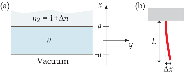
The setup is sketched in Fig. 1a; it is essentially the same as Fig. 2.1 in Ref. [5]. The beam is propagating into the plane, in the $z$ direction. On the lower side of the slab ($x<-a$) we assume vacuum (or air), with refractive index $n_{0}=1$. On the upper side ($x>a$), we assume that there is a dilute medium, extending to $x=\infty$, with refractive index $n_{2}=1+\Delta n$, $\Delta n\ll 1$. When light propagates through the fiber, there will thus be an imbalance in the surface force densities on the lower and upper surfaces. Let use choose a TE mode (following the notation in Ref. [5]). It means that the electric field has only an $y$ component different from zero, ${\bf E}=(0,E_{y},0)$. In the dielectric boundary layers located around $x=-a$ and $x=a$, the transverse force component is $f_{x}^{\mathrm{AM}}=-(\varepsilon_{0}/2)E_{y}^{2}\,d(n^{2})/dx$, yielding the respective surface force densities to be

We have here taken into account that the longitudinal component $E_{y}$ is continuous across the surfaces, and that $\langle{\tilde{E}^{2}_{y}}\rangle=\frac{1}{2}E^{2}_{y}$ where $\langle~\rangle$ is average over oscillations in time and the $z$ direction.

The net transverse surface force density is $\sigma_{x}=\sigma_{x}(-a)+\sigma_{x}(a)$. As $\Delta n$ is small, we can make use of the expression for $E_{y}^{2}$ corresponding to a symmetric fiber, thus with the assumption $n_{2}=1$. We get accordingly to first order in $\Delta n$

where now $E_{y}^{2}(a)$ refers to the symmetric situation. We see that for positive $\Delta n$, the surface force is directed downwards in Fig. 1a, i.e., in the negative $x$ direction. This is as it should be, as surface forces are always directed towards the optically thinner region at a dielectric surface.

The presence of $\sigma_{x}$ makes it possible to regard the fiber as an elastic rod exposed to a constant transverse load. Let us first, however, relate $\sigma_{x}$ to the total power $P$ in the fiber. For the TE mode we have, using the same notation as in Ref. [5],

Here $\kappa=\sqrt{n^{2}\omega^{2}/c^{2}-\beta^{2}}$ and $\xi=\sqrt{\beta^{2}-\omega^{2}/c^{2}}$, where $\beta$ lying in the interval $\omega/c\leq\beta\leq n\omega/c$ is the wave number component in the $z$ direction. The corresponding nondimensional transverse wave vectors are $u=\kappa a$, $w=\xi a$.

The electromagnetic boundary conditions, requiring that $dE_{y}/dx$ be continuous, yield the following equations:

with $m=0,1,2...$, while $u$ and $w$ are related via

From the above equations $\beta$ and $w$ can be calculated, and we can find the relationship between $P$ and the constant $A$ in Eq. (5) using formula (2.34) in Ref. [5]:

Recall that $P$ refers to the total power transmitted by the fiber. In the planar model, we have let $b$ denote the fiber width in the $y$ direction. The cross sectional area of the model fiber is thus $2ab$, and the power per unit length in the $y$ direction is $P/b$. Edge effects because of the finite value of $b$ are ignored. The transverse surface force density can now be expressed as

where we have defined

and used that the continuity of $dE_{y}/dx$ across the interface at $x=a$ implies that

For practical purposes it may be convenient to express $\Delta n$ in Eq. (9) in terms of the corresponding increase $\Delta\rho$ in material density. We can make use of the Clausius-Mossotti relation, which is a good approximation at least for nonpolar materials. We then get

Consider next the fiber as an elastic rod of rectangular cross section, clamped at one end ($z=0$) and free at the other end ($z=L$). For convenience we let the $z$ axis be horizontal. We choose $b=2a$, implying a square cross section of the fiber. The transverse load per unit length in the longitudinal direction is $\sigma_{x}b$ acting downwards in the negative $x$ direction. The governing equation for the elastic deflection is (we ignore gravity) $x^{\prime\prime\prime\prime}(z)=\sigma_{x}b/(EI)$, where $E$ is Young’s modulus and $I=b^{4}/12$ the moment of inertia of the cross-sectional area about its centroidal axis [7]. The solution of the governing equation is

The deflection at the tip, called simply $\Delta x$, is thus

We can now calculate the perturbation $\Delta n$ required to produce a relative deflection $\Delta x/L$ at the tip:

In order to obtain an order of magnitude estimate for the required difference in $n$ in order to yield a prescribed value for $\Delta x$ we insert numerical values that are appropriate for a low-intensity laser beam in a fiber (the numbers are typical, and the same as used in Ref. [6]): $\lambda=650$nm, $P=6.4$mW, $L=1.5$mm, $b=2a=450$nm.

For the eigenvalues of the transverse wave number $\beta$ (or, equivalently, $n_{e}$), corresponding to the guiding modes of the planar fiber, we use again the solutions for the symmetrical situations, since corrections to this only enter beyond leading order in $\Delta n$. Following [5], the eigenvalue of index $m=0,1,2,...$ solves

where $v={\textstyle\frac{\omega a}{c}}\sqrt{n^{2}-1}$ and $b=(n_{e}^{2}-1)/(n^{2}-1)$. With the current numbers there are only two modes, $n_{e,0}=1.3635$ and $n_{e,1}=1.1072$.

As an example, assume now we desire a lateral displacement $\Delta x=15~\upmu$m. With the above numbers we find that the required $\Delta n$ is only $5.5\cdot 10^{-4}$ for $m=0$ and $1.6\cdot 10^{-4}$ for $m=1$. Minor mechanical defects from production could easily give rise to changes in the reflective index of this magnitude. While the planar model is likely to underestimate the required $\Delta n$ slightly compared to a circular fiber, as an order of magnitude estimate it demonstrates the feasibility of the scheme.

Regard now a slightly more realistic model where the slab has a layer of slightly higher refractive index on one side. The geometry is as considered in Fig. 2 where the slab, still of width $2a$ and refractive index $n$, has refractive index raised by $\Delta n$ in a layer of thickness $\Delta a$. Again we consider the TE mode, whose solution for the electric field component $E_{y}$ is written [in layers (3) to (0) from top to bottom]

where $\Delta u=\kappa\Delta a,\Delta v=\kappa^{\prime}\Delta a$, $\phi$ and $\psi$ are unknown phase angles and $\kappa^{\prime 2}=(n+\Delta n)^{2}k^{2}-\beta^{2}\approx\kappa^{2}+2nk^{2}\Delta n$. The net surface force per unit area is now given by $\sigma_{x}=-(\varepsilon_{0}/2)\left.E_{y}^{2}(x)\right|_{x=-a}^{x=a}$.

To leading order in $\Delta n$ we may again use the relation (8) for $A$, and $\cos^{2}(u+\phi)$ is again given by equation (11).

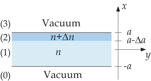
From continuity of $dE_{y}/dx$ at $x=a$ it follows that $\cos^{2}(\Delta v-\psi)=\kappa^{\prime 2}/(\xi^{2}+\kappa^{\prime 2})$, that is,

Similarly, from the condition of continuity of $dE_{y}/dx$ at $x=a-\Delta a$ we derive that, to linear order in $\Delta n$ we have

Thus we find with some calculation that the surface force per unit area may be written as

We may express $\cos^{2}\psi$ by means of the parameter $\Delta u$ by using the equation of continuity of $dE_{y}/dx$ at $x=a$, which may be written $\psi=-\arctan(\xi/\kappa)+\Delta v-m\pi$, $m=0,1,...$, to derive the relation, valid to leading order in $\Delta n$:

When $\Delta n$ is small we may use the same eigenvalues of $n_{e}$ as before.

Assuming once again that a displacement of $\Delta x=15\upmu$m is sought, figure 3a shows how the required $\Delta n$ changes with varying values of $\Delta a/a$. For the $m=0$ mode somewhat higher values of $\Delta n$ when $\Delta a/a$ is small. This is because $\sigma_{x}\propto\Delta n\Delta a$ as $\Delta a\to 0$. The required $\Delta n$ remains small, however, as long as the layer of slightly increased $n$ is non-vanishing. For $\Delta n>1\%$ for example, $\Delta a/a$ must be smaller than about $0.035$ to achieve the observed deflection.

The surface force density $\sigma_{x}/\Delta n$ to leading order is plotted as a function of $\Delta a/a$ in Fig. 3b. As in the simplest model of Fig. 1 the force is directed downward when $\Delta a/a$ is smaller than approximately unity. In the present example it is reasonable to assume that it is a small number compared to $1$. We have performed the calculation also using different laser wavelengths, in which case the graph of Fig. 3b looks qualitatively similar, but the abscissa is rescaled. Since the point where the force density changes sign (about $\Delta a/a=0.75$ in Fig. 3b) then moves along the abscissa, it is possible to change the sign of the force by changing the optical frequency, provided $\Delta a/a$ is chosen carefully.

The recent experiment of She et al. [6] appears to be a natural example of application for the present theory. This experiment tested precisely the sideways motion of a vertical fiber when transmitted by a laser beam. Whereas the authors actually related their observations to the Abraham-Minkowski problem mentioned above, we do no think that such a conclusion is right, and one of us has discussed this issue in more detail elsewhere [8]. In the experiment [6] one side of the fiber was slightly harder than the other from fabrication [9], and it is natural to suggest that this could have given rise to an appreciable $\Delta n$.

Noting how even very small $\Delta n$ can cause deflections of the magnitude observed, and how the surface force depends on the geometry of the hardened layer in a nontrivial way, it is much more likely in our opinion that all the observed transverse deviations reported in [6] were due to the force ${\bf f}^{\mathrm{AM}}$. As such the experiment is a striking demonstration of the theory presented herein. To ease comparison, our numerical examples above used data taken from the experiment [6], including a deflection in the order of $15\upmu$m. A change in the refractive index on one side of the fiber in the order of less than $1\%$ is shown to be sufficient to produce deflections of such magnitude.

In conclusion, only a minute change in the refractive index, around $10^{-3}$, in a layer on on one side of an optical fiber of centimetre length and micron scale cross-section is sufficient to produce an appreciable transverse deflection of the fibre. A tailored fiber of this kind, where $\Delta n$ is prescribed accurately, should provide the possibility to bend fibers in a controlled and predictable way. Because the lateral force acting on the fiber depends on the laser frequency in a non-trivial way, it would moreover be possible to design a fiber which bends one way at one frequency, and changes direction of movement when a different frequency is used. The force can be used to carry a small load and one can envisage uses within micro- and nano robotics.

Acknowledgment. I. B. thanks Weilong She for correspondence.

References

- [1] I. Brevik, Physics Reports 52, 133 (1979); cf. also the related article I. Brevik, Phys. Rev. B 33, 1058 (1986).
- [2] E. A. Hinds and S. M. Barnett, Phys. Rev. Lett. 102, 050403 (2009).
- [3] R. N. C. Pfeifer et al., Rev. Mod. Phys. 79, 1197 (2007).
- [4] C. Møller, The Theory of Relativity, 2nd ed. (Clarendon Press, Oxford, 1972), Ch. 7.
- [5] K. Okamoto, Fundamentals of Optical Waveguides (Academic Press, London, 2000).
- [6] W. She, J. Yu, and R. Feng, Phys. Rev. Lett. 101, 243601 (2008). See also Physical Review Focus, 10 December 2008.
- [7] L. D. Landau and E. M. Lifshitz, Theory of Elasticity (Pergamon Press, Oxford, 1970).
- [8] I. Brevik, Phys. Rev. Lett. 103, 219301 (2009); Reply: ibid. 103, 219302 (2009).
- [9] W. She, personal communication.