Matrix Graph Grammars: Transformation of Restrictions

Graph transformation [7, 24] is becoming increasingly popular in order to describe system behavior due to its graphical, declarative and formal nature. For example, it has been used to describe the operational semantics of Domain Specific Visual Languages (DSVLs, [14]), taking the advantage that it is possible to use the concrete syntax of the DSVL in the rules which then become more intuitive to the designer.

The main formalization of graph transformation is the so-called algebraic approach [7], which uses category theory in order to express the rewriting step. Prominent examples of this approach are the double [3, 7] and single [5] pushout (DPO and SPO) which have developed interesting analysis techniques, for example to check sequential and parallel independence between pairs of rules [7, 24] or the calculation of critical pairs [10, 13].

Frequently, graph transformation rules are equipped with application conditions (ACs) [6, 7, 11], stating extra (in addition to the left hand side) positive and negative conditions that the host graph should satisfy for the rule to be applicable. The algebraic approach has proposed a kind of ACs with predefined diagrams (i.e. graphs and morphisms making the condition) and quantifiers regarding the existence or not of matchings of the different graphs of the constraint in the host graph [6, 7]. Most analysis techniques for plain rules (without ACs) have to be adapted then for rules with ACs (see e.g. [13] for critical pairs with negative ACs). Moreover, different adaptations may be needed for different kinds of ACs. Thus, a uniform approach to analyze rules with arbitrary ACs would be very useful.

In previous works [15, 16, 17, 19] we developed a framework (Matrix Graph Grammars, MGGs) for the transformation of simple digraphs. Simple digraphs and their transformation rules can be represented using Boolean matrices and vectors. Thus, the rewriting can be expressed using Boolean operators only. One important point is that, as a difference from other approaches, we explicitly represent the rule dynamics (addition and deletion of elements) instead of only the static parts (rule pre and postconditions). This point of view enables new analysis techniques, such as for example checking independence of a sequence of arbitrary length and a permutation of it, or to obtain the smallest graph able to fire a sequence. On the theoretical side, our formalization of graph transformation introduces concepts from many branches of mathematics like Boolean algebra, group theory, functional analysis, tensor algebra and logics [19, 20, 21]. This wealth of available mathematical results opens the door to new analysis methods not developed so far, like sequential independence and explicit parallelism not limited to pairs of sequences, applicability, graph congruence and reachability. On the practical side, the implementations of our analysis techniques, being based on Boolean algebra manipulations, are expected to have a good performance.

In MGGs we do not only consider the elements that must be present in order to apply a production (left hand side, LHS, also known as certainty part) but also those elements that potentially prevent its application (also known as nihil or nihilation part). Refer to [22] in which, besides this, application conditions and graph constraints are studied for the MGG approach. The present contribution is a continuation of [22] where a comparison with related work can also be found. We shall tackle pre and postconditions, their transformation, the sequential version of these results and multidigraph rewriting.

We work with simple digraphs which we represent as $G=(M,V)$, where $M$ is a Boolean matrix for edges (the graph adjacency matrix) and $V$ a Boolean vector for vertices or nodes.¹¹ 1 The vector for nodes is necessary because in MGG nodes can be added and deleted, and thus we mark the existing nodes with a $1$ in the corresponding position of the vector. The left of Fig. 1 shows a graph representing a production system made up of a machine (controlled by an operator) which consumes and produces pieces through conveyors. Self loops in operators and machines indicate that they are busy.

Well-formedness of graphs (i.e. absence of dangling edges) can be checked by verifying the identity $\left\|\left(M\vee M^{t}\right)\odot\overline{V}\right\|_{1}=0$, where $\odot$ is the Boolean matrix product,²² 2 The Boolean matrix product is like the regular matrix product, but with and and or instead of multiplication and addition. $M^{t}$ is the transpose of the matrix $M$, $\overline{V}$ is the negation of the nodes vector $V$, and $\|\cdot\|_{1}$ is an operation (a norm, actually) that results in the or of all the components of the vector. We call this property compatibility (refer to [15]). Note that $M\odot\overline{V}$ results in a vector that contains a 1 in position $i$ when there is an outgoing edge from node $i$ to a non-existing node. A similar expression with the transpose of $M$ is used to check for incoming edges.

A type is assigned to each node in $G=(M,V)$ by a function from the set of nodes $|V|$ to a set of types $T$, $\lambda\colon|V|\rightarrow T$. Sets will be represented by $|\cdot|$. In Fig. 1 types are represented as an extra column in the matrices, where the numbers before the colon distinguish elements of the same type. It is just a visual aid. For edges we use the types of their source and target nodes. A typed simple digraph is $G_{T}=(G,\lambda)$. From now on we shall assume typed graphs and shall drop the $T$ subindex.

A production or grammar rule $p:L\rightarrow R$ is a morphism of typed simple digraphs, which is defined as a mapping that transforms $L$ in $R$ with the restriction that the type of the image must be equal to the type of the source element.³³ 3 We shall come back to this topic in Sec. 6. More explicitly, $f=(f_{V},f_{E})\colon G_{1}\rightarrow G_{2}$ being $f_{V}$ and $f_{E}$ partial injective mappings $f_{V}\colon|V_{1}|\rightarrow|V_{2}|$, $f_{E}\colon|M_{1}|\rightarrow|M_{2}|$ such that $\forall v\in Dom(f_{V}),\>\lambda_{1}(v)=\lambda_{2}(f_{V}(v))$ and $\forall e=(n,m)\in Dom(f_{E}),\>f_{E}(e)=f_{E}(n,m)=(f_{V}(n),f_{V}(m))$, where $Dom$ stands for domain, $E$ for edges and $V$ for vertices.

A production $p:L\rightarrow R$ is statically represented as $p=(L,R)=\left(\left(L^{E},L^{V},\lambda^{L}\right),\left(R^{E},R^{V},\lambda^{R}\right)\right)$. The matrices and vectors of these graphs are arranged so that the elements identified by morphism $p$ match (this is called completion, see below). Alternatively, a production adds and deletes nodes and edges, therefore they can be dynamically represented by encoding the rule’s LHS together with matrices and vectors representing the addition and deletion of edges and nodes:⁴⁴ 4 We call such matrices and vectors $e$ for “erase” and $r$ for “restock”. $p=(L,e,r)=\left(\left(L^{E},L^{V},\lambda^{L}\right),e^{E},r^{E},e^{V},r^{V},\lambda^{r}\right)$, where $\lambda^{r}$ contains the types of the new nodes, $e^{E}$ and $e^{V}$ are the deletion Boolean matrix and vector, $r^{E}$ and $r^{V}$ are the addition Boolean matrix and vector. They have a 1 in the position where the element is to be deleted or added, respectively. The output of rule $p$ is calculated by the Boolean formula $R=p(L)=r\vee\overline{e}\,L$, which applies both to nodes and edges.⁵⁵ 5 The and symbol $\wedge$ is usually omitted in formulae, so $R=p(L)=r\vee\overline{e}\wedge L$ with precedence of $\wedge$ over $\vee$.

In order to operate with the matrix representation of graphs of different sizes, an operation called completion adds extra rows and columns with zeros to matrices and vectors, and rearranges rows and columns so that the identified edges and nodes of the two graphs match. For example, in Fig. 2, if we need to operate $L^{E}$ and $R^{E}$, completion adds a fourth $0$-row and fourth $0$-column to $R^{E}$. No further modification is needed because the rest of the elements have the right types and are placed properly.⁶⁶ 6 In the present contribution we shall assume that completion is being performed somehow. This is closely related to non-determinism. The reader is referred to [21] for further details.

With the purpose of considering the elements in the host graph that disable a rule application, we extend the notation for rules with a new simple digraph $K$, which specifies the two kinds of forbidden edges: Those incident to nodes which are going to be erased and any edge added by the rule (which cannot be added twice, since we are dealing with simple digraphs). $K$ has non-zero elements in positions corresponding to newly added edges, and to non-deleted edges incident to deleted nodes. Matrices are derived in the following order: $\left(L,R\right)\mapsto\left(e,r\right)\mapsto K$. Thus, a rule is statically determined by its LHS and RHS $p=\left(L,R\right)$, from which it is possible to give a dynamic definition $p=\left(L,e,r\right)$, with $e=L\overline{R}$ and $r=R\overline{L}$, to end up with a full specification including its environmental behavior $p=\left(L,K,e,r\right)$. No extra effort is needed from the grammar designer because $K$ can be automatically calculated: $K=p(\overline{D})$, with $D=\overline{e^{V}}\otimes\overline{e^{V}}^{\,t}$.⁷⁷ 7 Symbol $\otimes$ denotes the tensor or Kronecker product, which sums up the covariant and contravariant parts and multiplies every element of the first vector by the whole second vector. The evolution of the nihilation matrix (what elements can not appear in the RHS) – call it $Q$ – is given by the inverse of the production: $(R,Q)=\left(p(L),p^{-1}(K)\right)=\left(r\vee\overline{e}L,e\vee\overline{r}K\right)$. See [22] for more details.

Inspired by the Dirac or bra-ket notation [2] we split the static part (initial state, $L$) from the dynamics (element addition and deletion, $p$): $R=p(L)=\left\langle L,p\right\rangle$. The ket operators (those to the right side of the bra-ket) can be moved to the bra (left hand side) by using their adjoints.

Matching is the operation of identifying the LHS of a rule inside a host graph. Given a rule $p:L\rightarrow R$ and a simple digraph $G$, any total injective⁸⁸ 8 MGG considers only injective matches. morphism $m:L\rightarrow G$ is a match for $p$ in $G$, thus it is one of the ways of completing $L$ in $G$. Besides, we shall consider the elements that must not be present.

Given the grammar rule $p:L\rightarrow R$ and the graph $G=(G^{E},G^{V})$, $d=\left(p,m\right)$ is called a direct derivation with $m=\left(m_{L},m_{K}\right)$ and result $H=p^{*}\left(G\right)$ if the following conditions are satisfied:

1. 1.

   There exist total injective morphisms $m_{L}:L\rightarrow G$ and $m_{K}:K\rightarrow\overline{G}$ with $m_{L}(n)=m_{K}(n)$, $\forall n\in L^{V}$.

2. 2.

   The match $m_{L}$ induces a completion of $L$ in $G$. Matrices $e$ and $r$ are then completed in the same way to yield $e^{*}$ and $r^{*}$. The output graph is calculated as $H=p^{*}(G)=r^{*}\vee\overline{e^{*}}G$.

The negation when applied to graphs alone (not specifying the nodes) – e.g. $\overline{G}$ in the first condition above – will be carried out just on edges. Notice that in particular the first condition above guarantees that $L$ and $K$ will be applied to the same nodes in the host graph $G$.

In direct derivations dangling edges can occur because the nihilation matrix only considers edges incident to nodes appearing in the rule’s LHS and not in the whole host graph. In MGG an operator $T_{\varepsilon}$ takes care of dangling edges which are deleted by adding a preproduction (known as $\varepsilon-$production) before the original rule. Refer to [15, 16]. Thus, rule $p$ is transformed into the sequence $p;p_{\varepsilon}$, where $p_{\varepsilon}$ deletes the dangling edges and $p$ remains unaltered.

There are occasions in which two or more productions should be matched to the same nodes. This is achieved with the marking operator $T_{\mu}$ introduced in Chap. 6 in [19]. A grammar rule and its associated $\varepsilon$-production is one example and we shall find more in future sections.

In [15, 16, 17, 19] some analysis techniques for MGGs have been developed which we shall skim through. One important feature of MGG is that sequences of rules can be analyzed independently to some extent of any host graph. A rule sequence is represented by $s_{n}=p_{n};\ldots;p_{1}$ where application is from right to left, i.e. $p_{1}$ is applied first. For its analysis, the sequence is completed by identifying the nodes across rules which are assumed to be mapped to the same node in the host graph.

Once the sequence is completed, sequence coherence [15, 19, 20] allows us to know if, for the given identification, the sequence is potentially applicable, i.e. if no rule disturbs the application of those following it. The formula for coherence results in a matrix and a vector (which can be interpreted as a graph) with the problematic elements. If the sequence is coherent, both should be zero; if not, they contain the problematic elements. A coherent sequence is compatible if its application produces a simple digraph. That is, no dangling edges are produced in intermediate steps.

Given a completed sequence, the minimal initial digraph (MID) is the smallest graph that permits the application of such sequence. Conversely, the negative initial digraph (NID) contains all elements that should not be present in the host graph for the sequence to be applicable. In this way, the NID is a graph that should be found in $\overline{G}$ for the sequence to be applicable (i.e. none of its edges can be found in $G$). See Sec. 6 in [20] or Chaps. 5 and 6 in [19].

Other concepts we developed aim at checking sequential independence (same result) between a sequence and a permutation of it. G-Congruence detects if two sequences, one permutation of the other, have the same MID and NID. It returns two matrices and two vectors, representing two graphs which are the differences between the MIDs and NIDs of each sequence, respectively. Thus if zero, the sequences have the same MID and NID. Two coherent and compatible completed sequences that are G-congruent are sequentially independent. See Sec. 7 in [20] or Chap. 7 in [19].

In this section we shall brush up on application conditions (ACs) as introduced for MGG in [22] with non-fixed diagrams and quantifiers. For the quantification, a full-fledged monadic second order logic⁹⁹ 9 MSOL, see e.g. [4]. formula is used. One of the contributions in [22] is that a rule with an AC can be transformed into (sequences of) plain rules by adding the positive information to the left hand side of the production and the negative to the nihilation matrix.

A diagram $\mathfrak{d}$ is a set of simple digraphs $\{A^{i}\}_{i\in I}$ and a set of partial injective morphisms $\{d_{k}\}_{k\in K}$ with $d_{k}:A^{i}\rightarrow A^{j}$. The diagram $\mathfrak{d}$ is well defined if every cycle of morphisms commute. $GC=\big(\mathfrak{d}=(\{A^{i}\}_{i\in I},\{d_{j}\}_{j\in J}),\mathfrak{f}\big)$ is a graph constraint where $\mathfrak{d}$ is a well defined diagram and $\mathfrak{f}$ a sentence with variables in $\{A^{i}\}_{i\in I}$ and predicates $P$ and $Q$. See eqs. (1) and (2). Formulae are restricted to have no free variables except for the default second argument of predicates $P$ and $Q$, which is the host graph $G$ in which we evaluate the GC. GC formulae are made up of expressions about graph inclusions. The predicates $P$ and $Q$ are given by:

where predicate $F(m,X)$ states that element $m$ (a node or an edge) is in graph $X$. Predicate $P(X^{1},X^{2})$ means that graph $X^{1}$ is included in $X^{2}$. Predicate $Q(X^{1},X^{2})$ asserts that there is a partial morphism between $X^{1}$ and $X^{2}$, which is defined on at least one edge ($e$ ranges over all edges). The notation (syntax) will be simplified by making the host graph $G$ the default second argument for predicates $P$ and $Q$. Besides, it will be assumed that by default total morphisms are demanded: Unless otherwise stated predicate $P$ is assumed. We take the convention that negations in abbreviations apply to the predicate (e.g. $\exists A[\overline{A}]\equiv\exists A[\overline{P}(A,G)]$) and not the negation of the graph’s adjacency matrix.

Given the rule $p:L\rightarrow R$ with nihilation matrix $K$, an application condition AC (over the free variable $G$) is a GC satisfying:

1. 1.

   $\exists!i,j$ such that $A^{i}=L$ and $A^{j}=K$.

2. 2.

   $\exists!k$ such that $A^{k}=G$ is the only free variable.

3. 3.

   $\mathfrak{f}$ must demand the existence of $L$ in $G$ and the existence of $K$ in $\overline{G}$.

For simplicity, we usually do not explicitly show the condition 3 in the formulae of ACs, nor the nihilation matrix $K$ in the diagram which are existentially quantified before any other graph of the AC. Notice that the rule’s LHS and its nihilation matrix can be interpreted as the minimal AC a rule can have. For technical reasons addressed in Sec. 5 (related to converting pre into postconditions) we assume that morphisms $d_{i}$ in the diagram do not have codomain $L$ or $K$. This is easily solved as we may always use their inverses due to $d_{i}$’s injectiveness.

It is possible to embed arbitrary ACs into rules by including the positive and negative conditions in $L$ and $K$, respectively. Intuitively: “MGG + AC = MGG” and “MGG + GC = MGG”. In [22] two basic operations are introduced: closure – $\widecheck{T}$ – that transforms universal into existential quantifiers, and decomposition – $\widehat{T}$ – that transforms partial morphisms into total morphisms. Notice that a match is an existentially quantified total morphism. It is proved in [22] that any AC can be embedded into its corresponding direct derivation. This is achieved by transforming the AC into some sequences of productions. There are four basic types of ACs/GCs. Let $GC=\left(\mathfrak{d},\mathfrak{f}\right)$ be a graph constraint with diagram $\mathfrak{d}=\{A\}$ and consider the associated production $p:L\to R$. The case $\mathfrak{f}=\exists A[A]$ is just the matching of $A$ in the host graph $G$. It is equivalent to the sequence $p;id_{A}$, where $id_{A}$ has $A$ as LHS and RHS, so it simply demands its existence in $G$. We introduce the operator $T_{A}$ that replaces $p$ by $p;id_{A}$ and leaves the diagram and the formula unaltered. If the formula $\mathfrak{f}=\forall A[A]$ is considered, we can reduce it to a sequence of matchings via the closure operator $\widecheck{T}_{A}$ whose result is:

with $A^{i}\cong A$, $d_{ij}\not\in iso(A^{i},A^{j})$,¹⁰¹⁰ 10 $iso(A,G)=\{f\colon A\rightarrow G\;|\;f$ is an isomorphism$\}$. $\widecheck{T}_{A}\left(AC\right)=AC^{\prime}=\left(\mathfrak{d}^{\prime},\mathfrak{f}^{\prime}\right)$ and $n=|par^{max}(A,G)|$.¹¹¹¹ 11 $par^{max}(A,G)=\{f\colon A\rightarrow G\;|\;f$ is a maximal non-empty partial morphism with $Dom(f)^{V}=A^{V}\}$. This is equivalent to the sequence $p;id_{A^{n}};\ldots;id_{A^{1}}$. If the application condition has formula $\mathfrak{f}=\exists A[Q(A)]$, we can proceed by defining the composition operator $\widehat{T}_{A}$ with action:

where $A^{i}$ contains a single edge of $A$ and $n$ is the number of edges of $A$. This is equivalent to the set of sequences $\left\{p;id_{A^{i}}\right\},i\in\{1,\ldots,n\}$.

Less evident are formulas of the form $\mathfrak{f}=\nexists A[A]=\forall A[\overline{A}]$. Fortunately, operators $\widecheck{T}$ and $\widehat{T}$ commute when composed so we can get along with the operator $\widetilde{T}_{A}=\widehat{T}_{A}\circ\widecheck{T}_{A}=\widecheck{T}_{A}\circ\widehat{T}_{A}$. The image of $\widetilde{T}$ on such ACs are given by:

An AC is said to be coherent if it is not a contradiction (false in all scenarios), compatible if, together with the rule’s actions, produces a simple digraph, and consistent if $\exists G$ host graph such that $G\models AC$¹²¹² 12 We shall say that the host graph $G$ satisfies $\exists A[A]$, written $G\models\exists A[A]$, if and only if $\exists f\in par^{max}(A,G)\>[f\in tot(A,G)]$, being $tot(A,G)=\{f:A\to G\;|\;f$ is a total morphism$\}\subseteq par^{max}(A,G)$. Also, $G$ satisfies $\forall A[A]$, writteni $G\models\forall A[A]$, if and only if $\forall f\in par^{max}(A,G)\>[f\in tot(A,G)]$. Usually we shall abuse of the notation and write $G\models GC$ instead. For more details, please refer to [22]. to which the production is applicable. As ACs can be transformed into equivalent (sets of) sequences, it is proved in [22] that coherence and compatibility of an AC is equivalent to coherence and compatibility of the associated (set of) sequence(s), respectively. Also, an AC is consistent if and only if its equivalent (set of) sequence(s) is applicable. Besides, all results and analysis techniques developed for MGG can be applied to sequences with ACs. Some examples follow:

• •

  As a sequence is applicable if and only if it is coherent and compatible (see Sec 6.4 in [19]) then an AC is consistent if and only if it is coherent and compatible.

• •

  Sequential independence allows us to delay or advance the constraints inside a sequence. As long as the productions do not modify the elements of the constraints, this is transformation of preconditions into postconditions. More on Sec. 5.

• •

  Initial digraph calculation solves the problem of finding a host graph that satisfies a given AC/GC. There are some limitations, though. For example it is necessary to limit the maximum number of nodes when dealing with universal quantifiers. This has no impact in some cases, for example when non-uniform MGG submodels are considered (see nodeless MGG in [21]).

• •

  Graph congruence characterizes sequences with the same initial digraph. Therefore it can be used to study when two GCs/ACs are equivalent for all morphisms or for some of them.

Summarizing, there are two basic results in [22]. First, it is always possible to embed an application condition into the LHS of the production or derivation. The left hand side $L$ of a production receives elements that must be found – $P(A,G)$ – and $K$ those whose presence is forbidden – $\overline{P}(A,G)$ –. Second, it is always possible to find a sequence or a set of sequences of plain productions whose behavior is equivalent to that of the production plus the application condition.

In this section we shall introduce postconditions and state some basic facts about them analogous to those for preconditions. We shall enlarge the notation by appending a left arrow on top of the conditions to indicate that they are preconditions and an upper right arrow for postconditions. Examples are $\stackrel{{\scriptstyle\leftarrow}}{{A}}$ for a precondition and $\stackrel{{\scriptstyle\rightarrow}}{{A}}$ for a postcondition. If it is clear from the context, arrows will be omitted.

Operators $T_{\stackrel{{\scriptstyle\rightarrow}}{{A}}},\widehat{T}_{\stackrel{{\scriptstyle\rightarrow}}{{A}}},\widecheck{T}_{\stackrel{{\scriptstyle\rightarrow}}{{A}}}$ and $\widetilde{T}_{\stackrel{{\scriptstyle\rightarrow}}{{A}}}$ are defined similarly for postconditions. The following proposition establishes an equivalence between the basic formulae (match, decomposition, closure and negative application condition) and certain sequences of productions.

The second case (closure) is very similar. We have to verify all potential appearances of $A$ in the image of the host graph because $\nexists A[\overline{A}]=\forall A[A]$. We proceed as in the first case but this time with a finite number of compositions: $\left(id_{A^{1}}\circ\ldots\circ id_{A^{m}}\circ p\right)(L)$.

For decomposition, $A$ is not found in the host graph if for some matching there is at least one missing edge. It is thus similar to matching but for a single edge. The way to proceed is to consider the set of sequences that appear in eq. (8). Negative application conditions (NACs) are the composition of eqs. (7) and (8). $\blacksquare$

One of the main points of the techniques available for preconditions is to analyze rules with ACs by translating them into sequences of flat rules, and then analyzing the sequences of flat rules instead.

A diagram $\mathfrak{d}$ is a graph where nodes are digraphs $A^{i}$ and edges are morphisms $d_{ij}$. There are $16$ possibilities for depth $1$ in a AC made up of a single element $A$, summarized in Table 1.

Elements in the same row for each pair of columns are related using equalities $\nexists A[A]=\forall A[\overline{A}]$ and $/\penalty\!\!\forall A[A]=\exists A[\overline{A}]$, so it is possible to reduce the study to cases (1*) – (4*) and (9*) – (12*). Identities $\overline{Q}(A)=P(A,\overline{G})$ and $Q(A)=\overline{P}(A,\overline{G})$ reduce (9*) – (12*) to formulae (1*) – (4*):

Proposition 4.2 considers the four basic cases which correspond to (1*) – (4*) in Table 1, showing that in fact they can all be reduced to matchings in the image of the host graph, i.e. to (1*) in Table 1, verifying the theorem.

Now we move on to the induction step which considers combinations of quantifiers. Well-definedness guarantees independence with respect to the order in which elements $A^{i}$ in the postcondition are selected. When there is a universal quantifier $\forall A$, according to eq. (7), elements of $A$ are replicated as many times as potential instances of $A$ can be found in the host graph. In order to continue the procedure we have to clone the rest of the diagram for each replica of $A$, except those graphs which are existentially quantified before $A$ in the formula. That is, if we have a formula $\exists B\forall A\exists C$ when performing the closure of $A$, we have to replicate $C$ as many times as $A$, but not $B$. Moreover $B$ has to be connected to each replica of $A$, preserving the identifications of the morphism $B\rightarrow A$. More in detail: When closure is applied to $A$, we iterate on all graphs $B_{j}$ in the diagram. There are three possibilities:

• •

  If $B_{j}$ is existentially quantified after $A$ – $\forall A...\exists B_{j}$ – then it is replicated as many times as $A$. Appropriate morphisms are created between each $A^{i}$ and $B^{i}_{j}$ if a morphism $d\colon A\rightarrow B$ existed. The new morphisms identify elements in $A^{i}$ and $B^{i}_{j}$ according to $d$. This permits finding different matches of $B_{j}$ for each $A^{i}$, some of which can be equal.¹³¹³ 13 If for example there are three instances of $A$ in the image of the host graph but only one of $B_{j}$, then the three replicas of $B$ are matched to the same part of $p(G)$.

• •

  If $B_{j}$ is existentially quantified before $A$ – $\exists B_{j}...\forall A$ – then it is not replicated, but just connected to each replica of $A$ if necessary. This ensures that a unique $B_{j}$ has to be found for each $A^{i}$. Moreover, the replication of $A$ has to preserve the shape of the original diagram. That is, if there is a morphism $d\colon B\rightarrow A$ then each $d_{i}\colon B\rightarrow A^{i}$ has to preserve the identifications of $d$ (this means that we take only those $A^{i}$ which preserve the structure of the diagram).

• •

  If $B_{j}$ is universally quantified (no matter if it is quantified before or after $A$), again it is replicated as many times as $A$. Afterwards, $B_{j}$ will itself need to be replicated due to its universality. The order in which these replications are performed is not relevant as $\forall A\forall B_{j}=\forall B_{j}\forall A$. $\blacksquare$

Previous theorem and the corollaries that follow heavily depend on the host graph and its image (through matching) so analysis techniques developed so far in MGG which are independent of the host graphs can not be applied. The “problem” is the universal quantifier. We can consider the initial digraph and dispose to some extent of the host graph and its image. This is related to the fact (Sec. 5) that it is possible to transform postconditions into equivalent preconditions.

Two applications of Th. 4.3 are the following corollaries that characterize coherence, compatibility and consistency of postconditions.

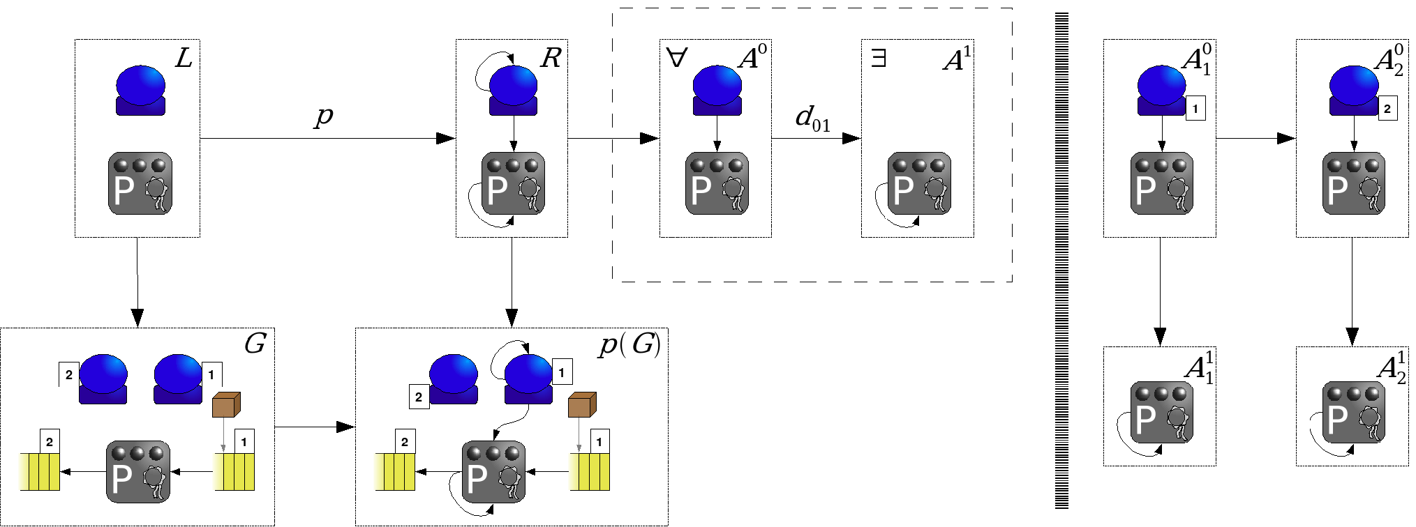
Once the formula has existentials only, we manipulate it to get rid of implications. Thus, we have $\exists A^{0}_{1}A^{0}_{2}A^{1}_{1}A^{1}_{2}[(\overline{A^{0}_{1}}\vee A^{1}_{1})\wedge(\overline{A^{0}_{2}}\vee A^{1}_{2})]=\exists A^{0}_{1}A^{0}_{2}A^{1}_{1}A^{1}_{2}[(\overline{A^{0}_{1}}\wedge\overline{A^{1}_{2}})\vee(\overline{A^{0}_{1}}\wedge A^{1}_{2})\vee(A^{1}_{1}\wedge\overline{A^{0}_{2}})\vee(A^{1}_{1}\wedge A^{1}_{2})]$. This leads to a set of four sequences: $\{(\overline{id}_{A^{0}_{1}};\overline{id}_{A^{0}_{2}}),(\overline{id}_{A^{0}_{1}};id_{A^{1}_{2}}),(id_{A^{1}_{1}};\overline{id}_{A^{0}_{2}}),(id_{A^{1}_{1}};id_{A^{1}_{2}})\}$. Thus, the graph $p(G)$ and the production satisfy the postcondition if and only if some sequence in the set is applicable to $p(G)$. $\blacksquare$

Something left undefined is the order of productions $id_{A^{i}}$ and $\overline{id}_{A^{i}}$ in the sequences. Consistency does not depend on the ordering of productions – as long as the first to be applied is production $p$ – because productions $id$ (and their negation) are sequentially independent (they do not add nor delete any edge or node). If they are not sequentially independent then there exists at least one inconsistency. This inconsistency can be detected using previous corollaries independently of the order of the productions.

In this section we give two different proofs that it is possible to transform preconditions into equivalent postconditions and back again. The first proof (sketched) makes use of category theory while the second relies on the characterizations of coherence, G-congruence and compatibility. To ease exposition we shall focus on the certainty part only as the nihilation part would follow using the inverse of the production.

We shall start with a case that can be addressed using equations (6) – (9), Th. 4.3 and Cor. 4.4: When the transformed postcondition for a given precondition does not change.¹⁴¹⁴ 14 This is not so unrealistic. For example, if the production preserves all elements appearing in the precondition. The question of whether it is always possible to transform a precondition into a postcondition – and back again – in this restricted case would be equivalent to asking for sequential independence of the production $p$ and the identities $id$ or $\overline{id}$:

where the sequence to the left of the equality corresponds to a precondition and the sequence to the right corresponds to its equivalent postcondition.

In general the production may act on elements that appear in the diagram of the precondition, spoiling sequential independence. Left and center of Fig. 5 -- in which the first basic AC (match) is considered -- suggest that the pre-to-post transformation is a categorical pushout¹⁵¹⁵ 15 The square $\left\{L,R,\stackrel{{\scriptstyle\leftarrow}}{{A}},\stackrel{{\scriptstyle\rightarrow}}{{A}}\right\}$ is a pushout where $p$, $L$, $d_{L}$, $R$ and $\stackrel{{\scriptstyle\leftarrow}}{{A}}$ are known and $\stackrel{{\scriptstyle\rightarrow}}{{A}}$, $p_{A}$ and $d_{L}$ need to be calculated. in the category of simple digraphs and partial morphisms.

Theorem 4.3 proves that any postcondition can be reduced to the match case. Besides, we can trivially consider total morphisms (instead of partial ones) by restricting the domain and the codomain of $p$ to the nodes in $\stackrel{{\scriptstyle\leftarrow}}{{A}}$. For the post-to-pre transformation we can either use pullbacks or pushouts plus the inverse of the production involved.

To see that precondition satisfaction is equivalent to postcondition satisfaction using category theory, we should check that the different pushouts can be constructed ($p^{*},p_{A},p^{*}_{A}$, etcetera) and that $d_{L}=m_{\stackrel{{\scriptstyle\leftarrow}}{{A}}}\circ m_{L}$ and $d^{*}_{L}=m_{\stackrel{{\scriptstyle\rightarrow}}{{A}}}\circ m^{*}_{L}$ (refer to Fig. 5). Although some topics remain untouched such as dangling edges, we shall not carry on with category theory.

Recall that $G$-congruence guarantees sameness of the initial digraph, which is what the sequence demands on the host graph. Therefore, all we have to do is to use $G$-congruence to check the differences in the two sequences:

However, before that we need to guarantee coherence and compatibility of both sequences (see the hypothesis of Th. 4 in [20]). Coherence gives rise to the following equation:

where $e$ and $r$ correspond to $p$, $e_{\stackrel{{\scriptstyle\leftarrow}}{{A}}}$ to $id_{\stackrel{{\scriptstyle\leftarrow}}{{A}}}$ and $r_{\stackrel{{\scriptstyle\rightarrow}}{{A}}}$ to $id_{\stackrel{{\scriptstyle\rightarrow}}{{A}}}$. Fortunately, $id$ is a production that does nothing, so from the dynamical point of view any conflict should come from $p$, i.e. $e_{\stackrel{{\scriptstyle\leftarrow}}{{A}}}=r_{\stackrel{{\scriptstyle\rightarrow}}{{A}}}=\mathbf{0}$ which has been used in the implication of eq. (12).

By consistency we have that $r\!\!\stackrel{{\scriptstyle\leftarrow}}{{A}}=\mathbf{0}$ so eq. (12) will be fulfilled if the postcondition is the precondition but erasing the elements that the production deletes. A similar reasoning for the nihil part tells us that we should add to the postcondition all those elements added by the production.

Compatibility can only be ruined by dangling edges. In Sec. 6.1 in [19] dangling edges are deleted transforming the production via the opeartor $T_{\varepsilon}$. This is proved to be equivalent to defining a sequence by appending a so-called $\varepsilon$-production. In essence the $\varepsilon$-production just deletes any dangling edge, thus keeping compatibility. This very same procedure can be applied now:

According to Prop. 5 and Th. 4 in [20], two compatible and coherent sequences are $G$-congruent if the following equation (adapted to our case) is fulfilled:

We have that $e_{\stackrel{{\scriptstyle\leftarrow}}{{A}}}=r_{\stackrel{{\scriptstyle\leftarrow}}{{A}}}=\mathbf{0}$. Also, $K_{\stackrel{{\scriptstyle\leftarrow}}{{A}}}=\mathbf{0}$ because $id_{\stackrel{{\scriptstyle\leftarrow}}{{A}}}$ acts on the certainty part and $\overline{e}r=r$ (see e.g. Prop. 4.1.4 in [24]). We are left with

which is guaranteed by compatibility: once $id_{\stackrel{{\scriptstyle\leftarrow}}{{A}}}$ is transformed into $id^{\phantom{i}\varepsilon}_{\stackrel{{\scriptstyle\leftarrow}}{{A}}}$ in eq. (13) there can not be any potential dangling edge, except those to be deleted by $p$ in the last step. $\blacksquare$

It is worth stressing the fact that the transformation between pre and postconditions preserve consistency of the application condition. We have seen in this section that $p$ not only acts on $L$ but on the whole precondition. We can therefore extend the notation:

Pre-to-post and post-to-pre transformations can affect the diagram and the formula. See the example below. There are two clear cases:

• •

  The application condition requires the graph to appear and the production deletes all its elements.

• •

  The application condition requires the graph not to appear and the production adds all its elements.

For a given application condition AC it is not necessarily true that $A=p^{-1};p(A)$ because some new elements may be added and some obsolete elements discarded. What we will get is an equivalent condition adapted to $p$ that holds whenever $A$ holds and fails to be true whenever $A$ is false.

Suppose we had a (redundant) graph $B$ made up of a single node $1$ with a self loop in the precondition and with formula $\stackrel{{\scriptstyle\leftarrow}}{{\mathfrak{f}}}=\exists AB[AB]$. The formula in the postcondition would still be $\stackrel{{\scriptstyle\rightarrow}}{{\mathfrak{f}}}=\exists A[A]$.

The opposite transformation, from postcondition into precondition, can be obtained by reverting the arrow, i.e. through $p^{-1}(A)$. More general schemes can be studied applying the same principles.

Let $\mathcal{A}=p^{-1}\circ p\left(\stackrel{{\scriptstyle\leftarrow}}{{A}}\right)$. If a pre-post-pre transformation is carried out, we will have $\stackrel{{\scriptstyle\leftarrow}}{{A}}\,\neq\mathcal{A}$ because edge (2,1) would be added to $\stackrel{{\scriptstyle\leftarrow}}{{A}}$. However, it is true that $\mathcal{A}=p^{-1}\circ p\left(\mathcal{A}\right)$.

Note that in fact $id_{\stackrel{{\scriptstyle\leftarrow}}{{A}}}$ and $p$ are sequentially independent if we limit ourselves to edges, so it would be possible to simply move the precondition to a postcondition as it is. Nonetheless, we have to consider nodes 1 and 2 as the common parts between $L$ and $\stackrel{{\scriptstyle\leftarrow}}{{A}}$. This is the same kind of restriction as the one illustrated in Fig. 6. $\blacksquare$

If the pre-post-pre transformation is thought of as an operator $T_{p}$ acting on application conditions, then it fulfills

where $id$ is the identity. The same would also be true for a post-pre-post transformation.

A possible interpretation of eq. (17) is that the definition of the application condition can vary from the natural one, according to the production under consideration. Pre-post-pre or post-pre-post transformations adjust application conditions to the corresponding production.

When defining diagrams some “practical problems” may turn up. For example, if the diagram $\mathfrak{d}=\left(L\stackrel{{\scriptstyle d_{L0}}}{{\rightarrow}}A^{0}\stackrel{{\scriptstyle d_{10}}}{{\leftarrow}}A^{1}\right)$ is considered then there are two potential problems:

1. 1.

   The direction in the arrow $A^{0}\leftarrow A^{1}$ is not the natural one. Nevertheless, injectiveness allows us to safely revert the arrow, $d_{01}=d^{-1}_{10}$.

2. 2.

   Even though we only formally state $d_{L0}$ and $d_{10}$, other morphisms naturally appear and need to be checked out, e.g. $d_{L1}:R\rightarrow A^{1}$. New morphisms should be considered if they relate at least one element.¹⁶¹⁶ 16 Otherwise stated: Any condition made up of $n$ graphs $A^{i}$ can be identified as the complete graph $K_{n}$, in which nodes are graphs $A^{i}$ and morphisms are $d_{ij}$. Whether this is a directed graph or not is a matter of taste (morphisms are injective).

In this section we touch on delocalization of graph constraints and application conditions as well as their equivalence. Also, we shall pave the way to multidigraph rewriting to be studied in detail in Sec. 7.

Let $s=p_{n};\ldots;p_{1}$ be a sequence of productions with their corresponding ACs. We have seen in Th. 4.3 that preconditions and postconditions are equivalent and in Th. 5.1 that they can be transformed into sequences of productions. As a precondition in $p_{i+1}$ is the same as a postcondition in $p_{i}$, we see that ACs can be moved arbitrarily inside a sequence.

Similarly, constraints set on the intermediate states of a derivation can be moved among them. A graph constraint GC set in the initial state $G$ to which a production $p$ is going to be applied is equivalent to the precondition

If the GC is set on the final state $H=p(G)$ to which the production $p$ has been applied, there is an equivalent postcondition:

In both cases the diagrams are given by the LHS or the RHS plus the diagram of the graph constraint. We call this property of application conditions and graph constraints delocalization.

We shall now address variable nodes which will be used to enhance MGG functionality to deal with multidigraphs. Graph transformation with variables is studied in [12]. We shall summarize the proposal in [12] and propound an alternative way to close the section.

If instead of nodes of fixed type variable, types are allowed we get a so called graph pattern. A rule scheme is just a production in which graphs are graph patterns. A substitution function $\iota$ specifies how variable names taking place in a production are substituted. A rule scheme $p$ is instantiated via substitution functions producing a particular production. For example, for substitution function $\iota$ we get $p^{\,\iota}$. The set of production instances for $p$ is defined as the set $\mathcal{I}(p)=\left\{p^{\,\iota}\;|\right.$ $\iota$ is a substitution$\left.\right\}$. The kernel of a graph $G$, $ker(G)$, is defined as the graph resulting when all variable nodes are removed. It might be the case that $ker(G)=\emptyset$.

The basic idea is to reduce any rule scheme to a set of rule instances. Note that it is not possible in general to generate $\mathcal{I}(p)$ because this set can be infinite. The way to proceed is not difficult:

1. 1.

   Find a match for the kernel of $L$.

2. 2.

   Induce a substitution $\iota$ such that the match for the kernel becomes a full match $m:L^{\iota}\rightarrow G$.

3. 3.

   Construct the instance $R^{\,\iota}$ and apply $p^{\,\iota}$ to get the direct derivation $G\stackrel{{\scriptstyle p^{\,\iota}}}{{\Longrightarrow}}H$.

As an alternative, we may extend the concept of type assignment. Recall from Sec. 2 that types are assigned by a function from the set of nodes $|V|$ of a simple digraph $G$ to some fixed set $T$ of types, $\lambda:|V|\to T$. Instead, we shall define

where $\mathcal{P}(T)$ is the power set¹⁷¹⁷ 17 The set of all subsets. of $T$ except for the empty set because we do not permit nodes without types.

When two matrices are operated, the types of a fixed node will be the intersection of the nodes operated. For example, suppose that we and two matrices $C=AB$ and that the (set of) nodes associated to the elements $a$ and $b$ are $\lambda(a)$ and $\lambda(b)$, respectively. Then, $\lambda(c)=\lambda(a)\cap\lambda(b)$. The operation would not be allowed in case $\lambda(c)=\lambda(a)\cap\lambda(b)=\emptyset$.

Let’s consider the graph constraint $GC_{0}=\left(\mathfrak{d}_{0},\mathfrak{f}_{0}\right)$, with $\mathfrak{d}_{0}$ the diagram depicted in Fig. 8 made up of the graphs $A^{0}$ and $A^{1}$, along with the formula $\mathfrak{f}_{0}=\forall A^{0}A^{1}[\overline{Q}(A^{0})\overline{Q}(A^{1})]$. This graph constraint is “edges must connect nodes and multinodes alternatively but no edge is allowed to be incident to two multinodes or to two simple nodes, including self-loops”.

In the graph $A^{0}$ of Fig. 8, $x$ and $y$ represent variable nodes while $a$ and $b$ in $A^{1}$ have a fixed type. We may think of $a$ and $b$ as variable nodes whose set of types has a single element. $\blacksquare$

In this section we show how MGG can deal with multidigraphs (directed graphs allowing multiple parallel edges) just by considering variable nodes. At first sight this might seem a hard task as MGG heavily depends on adjacency matrices. Adjacency matrices are well suited for simple digraphs but can not cope with parallel edges. This section can be thought of as a theoretical application of graph constraints and application conditions to Matrix Graph Grammars.

The idea is not difficult: A special kind of node (call it multinode in contrast to simple node) associated to every edge in the graph is introduced, i.e. edges in the multidigraph are substituted by multinodes in a simple digraph representation of the multidigraph. Graphically, multinodes will be represented by a filled square while normal nodes will appear as colored circles. See the example by the end of Sec. 6

Operations previously specified on edges now act on multinodes: Adding an edge is transformed into a multinode addition and edge deletion becomes multinode deletion. There are edges that link multinodes to their source and target simple nodes.

Some restrictions (application conditions) to be imposed on the actions that can be performed on multinodes exist, as well as on the shape or topology of permitted graphs (graph constraints). Not every possible graph with multinodes represents a multidigraph.

References

- [1] AGG, The Attributed Graph Grammar system. http://tfs.cs.tu-berlin.de/agg/.
- [2] Bra-ket notation intro: http://en.wikipedia.org/wiki/Bra-ket_notation
- [3] Corradini, A., Montanari, U., Rossi, F., Ehrig, H., Heckel, R., Löwe, M. 1999. Algebraic Approaches to Graph Transformation - Part I: Basic Concepts and Double Pushout Approach. In [24], pp.: 163-246
- [4] Courcelle, B. 1997. The expression of graph properties and graph transformations in monadic second-order logic. In [24], pp.: 313-400.
- [5] Ehrig, H., Heckel, R., Korff, M., Löwe, M., Ribeiro, L., Wagner, A., Corradini, A. 1999. Algebraic Approaches to Graph Transformation - Part II: Single Pushout Approach and Comparison with Double Pushout Approach. In [24], pp.: 247-312.
- [6] Ehrig, H., Ehrig, K., Habel, A., Pennemann, K.-H. Constraints and Application Conditions: From Graphs to High-Level Structures. Proc. ICGT’04. LNCS 3256, pp.: 287-303. Springer.
- [7] Ehrig, H., Ehrig, K., Prange, U., Taentzer, G. 2006. Fundamentals of Algebraic Graph Transformation. Springer.
- [8] Habel, A., Pennemann, K.-H. 2005. Nested Constraints and Application Conditions for High-Level Structures. In Formal Methods in Software and Systems Modeling, LNCS 3393, pp. 293-308. Springer.
- [9] Habel, A., Penneman, K.-H. 2009. Correctness of High-Level Transformation Systems Relative to Nested Conditions. Math. Struct. Comp. Science 19(2), pp.: 245–296.
- [10] Heckel, R., Küster, J.-M-., Taentzer, G. 2002. Confluence of typed attributed graph transformation systems. Proc. ICGT’02, LNCS 2505, pp. 161–176. Springer.
- [11] Heckel, R., Wagner, A. 1995. Ensuring consistency of conditional graph rewriting - a constructive approach., Electr. Notes Theor. Comput. Sci. (2).
- [12] Hoffman, B. 2005. Graph Transformation with Variables. In Graph Transformation, Vol. 3393/2005 of LNCS, pp. 101-115. Springer.
- [13] Lambers, L., Ehrig, H., Orejas, F. 2006. Conflict Detection for Graph Transformation with Negative Application Conditions. Proc ICGT’06, LNCS 4178, pp.: 61-76. Springer.
- [14] de Lara, J., Vangheluwe, H. 2004. Defining Visual Notations and Their Manipulation Through Meta-Modelling and Graph Transformation. Journal of Visual Languages and Computing. Special section on “Domain-Specific Modeling with Visual Languages”, Vol 15(3-4), pp.: 309-330. Elsevier Science.
- [15] Pérez Velasco, P. P., de Lara, J. 2006. Towards a New Algebraic Approach to Graph Transformation: Long Version. Tech. Rep. of the School of Comp. Sci., Univ. Autónoma Madrid. http://www.ii.uam.es/jlara/investigacion/techrep_03_06.pdf.
- [16] Pérez Velasco, P. P., de Lara, J. 2006. Matrix Approach to Graph Transformation: Matching and Sequences. Proc ICGT’06, LNCS 4178, pp.:122-137. Springer.
- [17] Pérez Velasco, P. P., de Lara, J. 2007. Using Matrix Graph Grammars for the Analysis of Behavioural Specifications: Sequential and Parallel Independence Proc. PROLE’07, pp.: 11-26. Electr. Notes Theor. Comput. Sci. (206). pp.:133–152. Elsevier.
- [18] Pérez Velasco, P. P., de Lara, J. 2007. Analysing Rules with Application Conditions using Matrix Graph Grammars. Graph Transformation for Verification and Concurrency (GTVC) workshop.
- [19] Pérez Velasco, P. P. 2009. Matrix Graph Grammars: An Algebraic Approach to Graph Dynamics. ISBN 978-3639212556. VDM Verlag. Also available as e-book at: http://www.mat2gra.info/ and arXiv:0801.1245v1.
- [20] Pérez Velasco, P. P., de Lara, J. 2009. A Reformulation of Matrix Graph Grammars with Boolean Complexes. The Electronic Journal of Combinatorics. Vol 16(1). R73. Available at: http://www.combinatorics.org/.
- [21] Pérez Velasco, P. P. 2009. Matrix Graph Grammars as a Model of Computation. Preliminary version available at arXiv:0905.1202v2.
- [22] Pérez Velasco, P. P., de Lara, J. 2010. Matrix Graph Grammars with Application Conditions. To appear in Fundamenta Informaticae. Also available at arXiv:0902.1809v2.
- [23] Rensink, A. 2004. Representing First-Order Logic Using Graphs. Proc. ICGT’04, LNCS 3256, pp.: 319-335. Springer.
- [24] Rozenberg, G. 1997. Handbook of Graph Grammars and Computing by Graph Transformation. Vol 1. World Scientific.