Training and Feedback Optimization for Multiuser MIMO Downlink
Abstract
We consider a MIMO fading broadcast channel where the fading channel coefficients are constant over time-frequency blocks that span a coherent time a coherence bandwidth. In closed-loop systems, channel state information at transmitter (CSIT) is acquired by the downlink training sent by the base station and an explicit feedback from each user terminal. In open-loop systems, CSIT is obtained by exploiting uplink training and channel reciprocity. We use a tight closed-form lower bound on the ergodic achievable rate in the presence of CSIT errors in order to optimize the overall system throughput, by taking explicitly into account the overhead due to channel estimation and channel state feedback. Based on three time-frequency block models inspired by actual systems, we provide some useful guidelines for the overall system optimization. In particular, digital (quantized) feedback is found to offer a substantial advantage over analog (unquantized) feedback.
1 SUPELEC, Gif-sur-Yvette, 91192, France
2 University of Minnesota, Minneapolis MN, 55455 USA
3 University of Southern California, Los Angeles CA, 90089 USA
Keywords: MIMO broadcast channel, Multiuser MIMO Downlink, Channel State Information Feedback, Channel Estimation.
I Introduction
The downlink of a wireless system with one Base Station (BS) with antennas and User Terminals (UTs) with a single antenna each is modeled by a MIMO Gaussian broadcast channel [1], defined by
| (1) |
for , where is the channel output at UT , is the corresponding Additive White Gaussian Noise (AWGN) process, is the vector of channel coefficients from the BS antenna array to the -th UT antenna and is the vector of channel input symbols transmitted by the BS, subject to the average power constraint (enforced for each channel use ). We denote the downlink signal-to-noise ratio (SNR) at each UT by . We assume a block fading model where the channel vectors remain constant over a coherence block of channel uses. The block length is related to two physical channel parameters, the coherence time and the coherence bandwidth by . For example, taking as typical values kHz and ms (from [2]), we obtain channel uses.
Albeit suboptimal, zero-forcing (ZF) beamforming with users captures the fundamental trend in terms of degrees of freedom (or “multiplexing gain”) [2]. Therefore, we focus on this case for its analytical tractability. In order to perform ZF beamforming (or any other multiuser MIMO precoding), the BS must have an accurate estimate of the downlink channel. Such information, referred to as the Channel State Information at the Transmitter (CSIT) is acquired by using downlink training and channel state feedback. On the one hand, in TDD systems with self-calibrating devices, owing to the fact that uplink and downlink take place in the same channel coherence bandwidth, CSIT can be acquired directly from the uplink pilot symbols. On the other hand, the uplink-downlink channel reciprocity does not hold in Frequency-Division Duplexing (FDD) systems where uplink and downlink take places in different widely separated frequency bands. This is also the case in Time-Division Duplexing (TDD) systems where uplink and downlink may time-share the same band but the non-linear devices are not self-calibrated and therefore induce non-reciprocal effects. In the latter case, an explicit CSIT feedback must be used. In any case, the rates achievable with ZF beamforming depend critically on the quality of the CSIT, however, high quality CSIT can be achieved by dedicating a significant amount of time resource to downlink training and (for FDD) to channel state feedback. It follows that there is a non-trivial tradeoff between the benefits of improving the CSIT and the overhead in channel estimation and feedback.
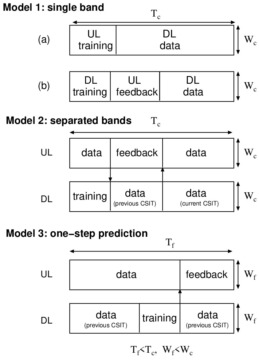
In this work, we determine the optimum fraction of resources that should be dedicated to training/feedback in several cases of interest. In particular, we consider three time-frequency block models depicted in Fig. 1. These models can be viewed as an idealization of the actual systems such as LTE [3] and aim at capturing the essential features. In Section III, we consider the optimization of the net spectral efficiency based on model 1 where both training and feedback consume “downlink” channel uses. This analysis applies naturally to TDD with or without reciprocity and FDD where downlink training and (uplink) feedback are performed in the same fading coherence block, via some hand-shaking protocol. In Section IV, we consider a different viewpoint based on models 2 and 3, in which the CSIT feedback consumes “uplink” channel uses. These models are more relevant to FDD systems. The question that we address is “how much uplink resource should one pay in order to achieve a certain downlink spectral efficiency?”. By solving the corresponding optimization problem, we characterize the uplink/downlink spectral efficiency region. At which point of this tradeoff region the system should operate is a function of the specific system requirements such as uplink/downlink traffic demands. For a fixed demand, the optimal operation point can be found adaptively. Further, we study the effect of temporally correlated fading channels and feedback delay where CSIT is obtained through a one-step prediction model (model 3). This corresponds to the case when the downlink block bandwidth and the block length are significantly shorter than the coherence bandwidth and the coherence interval , respectively. Finally, Section V presents some considerations for the case of users with some downlink scheduling and user selection [4]. This case is very relevant in practice, but its analysis has escaped so far a full closed-form characterization. Therefore, we provide results by combining Monte Carlo simulation and closed-form analysis.
The optimization of training has been studied in the context of point-to-point MIMO channels in the literature, e.g., [5, 6, 7, 8, 9]. In [5], the point-to-point MIMO communication is considered and only downlink training is addressed for the case of no CSIT and imperfect Channel State Information at the Receiver (CSIR). On the other hand, in [7], perfect CSIR is assumed and the resources to be used for channel feedback are investigated. In [8, 9] the model of [5] is extended to also incorporate quantized channel feedback and transmitter beamforming. Although the setup is quite similar to ours, the emphasis of [8, 9] on the asymptotic regime, where the number of antennas and are simultaneously taken to infinity, leads to rather different conclusions as compared to the present work. In [6], a MIMO broadcast with downlink training and perfect channel feedback (i.e., the BS is also able to view the received training symbols) is considered. It is shown that the sum rate achievable with a dirty paper coding-based strategy has a very similar form to the achievable rate expressions in [5], and thus many of the conclusions from [5] directly carry over. On the other hand, we consider the more practical case where there is imperfect feedback from each UT to the BS and also study achievable rates with ZF beamforming, which has lower complexity than dirty-paper coding. The present work is an extension of [10, 11], where the same optimization was investigated assuming that both downlink training and uplink feedback are performed within the same block (model 1). In this paper, we provide more complete guidelines on the overall system optimization for the various scenarios of interest.
II Channel State Estimation and Feedback
When the multiuser MIMO downlink is operated in a closed-loop mode, the CSIT is obtained through the following phases:
1) Common downlink training: shared pilot symbols (i.e.,
pilots per BS antenna) are transmitted on each channel coherence block
to allow all UTs to estimate their downlink channel vectors based on the observation
| (2) |
Using linear MMSE estimation, the per-coefficient estimation error variance is given by
| (3) |
2) Channel feedback: Each UT feeds back its channel estimation immediately after the training phase. We focus on the scenario where the feedback channel is modeled as an AWGN channel with the SNR , identical to the nominal downlink SNR. Because UT’s are assumed to access the feedback channel orthogonally, a total of channel symbols translates into feedback channel uses per UT. Different feedback strategies are described in Section III.
The BS obtains the channel state matrix based on the training/feedback information. Errors in the CSIT available to the BS stems from two sources: the channel estimation error during the common training phase, and the distortion incurred during the feedback phase. Then, the BS computes the ZF beamforming vector to be a unit-norm vector orthogonal to the subspace for all . In this case, the ergodic rate achievable by UT with equal-power allocation across UT’s and Gaussian random coding is given by:
| (4) |
assuming each UT is aware of its received signal-to-interference plus noise ratio (SINR).11 1 Such knowledge can be acquired through an additional dedicated training round as discussed in [12]. This training round does not significantly affect the present work, and thus is ignored for the sake of simplicity. The residual interference due to non-zero “leakage” coefficients decreases the achievable rate. In [12], it is shown that the rate in (4) is tightly lower-bounded by
| (5) |
where is the rate achievable with perfect CSIT and denotes the rate gap, given in closed form by
| (6) |
Assuming that the channel statistics are symmetric over users and space, , and do not depend on , therefore the subscript will be omitted in the following. The rate gap depends on , and the training/feedback strategy and will be generally denoted by the function . Explicit expressions are found in [12] for the cases addressed in this paper.
III Joint Optimization of Training and Feedback
In this section, we focus on model 1 of Fig. 1 where training and CSIT feedback consume downlink channel uses. Model 1 (a) refers to the TDD system exploiting the channel reciprocity, while model 1 (b) refers to either the TDD without reciprocity or the FDD system in which the downlink training and the feedback are performed in the same fading coherence block. In both cases, the maximization of the net downlink spectral efficiency is formulated as
| (7) |
It is convenient to consider the maximization in two steps, by writing:
| (8) |
Furthermore, the rate gap can be put in the general form (see [12])
| (9) |
where the function depends on the feedback strategy and shall be specified later. Because the first multiplicative term is constant when , the inner maximization corresponds to minimization of the function , subject to the constraint . Letting denote the solution of the inner maximization in (8), we can solve the outer maximization by searching for the optimal value .
III-A TDD with channel reciprocity
When channel reciprocity holds, open-loop CSIT estimation can be obtained from the uplink pilot symbols. In this case, the amount of uplink training can be optimized as a special case of (8) where no CSIT feedback is used.22 2 Note that a similar optimization is considered in [13], although in that work analysis of this optimization is not performed. In [12, Remark 4.2], the rate gap for a TDD system that uses uplink training symbols is given by:
| (10) |
which corresponds to with . Plugging this into (7), we maximize the net spectral efficiency given by
| (11) |
Because is concave in , the optimal can be found by numerically solving for where
| (12) |
Although a closed-form solution for cannot be found, we can study the scaling of the optimal with the system parameters. It is not difficult to see that the derivative in (12) is upperbounded by , where
| (13) |
The concavity of implies that the solution of the equation is an upper bound to the optimal value . Solving for , we find
| (14) |
Furthermore, when the rate gap is small such that (which becomes accurate for large ), the upperbound also becomes a very good approximation.
Two interesting behaviors are obtained from (21): 1) for a fixed SNR (i.e., constant ) increases as as ; 2) for a fixed block length , decreases as for large SNR, or equivalently, it decreases as since for large SNR.
Next, we examine the impact of on the net achievable rate. By the definition of we have:
| (15) |
The rate gap with respect to can therefore be upper bounded as:
| (16) | ||||
| (17) | ||||
| (18) |
where the final inequality is reached by dropping the last term in (17) and using . Thus, the gap to a perfect CSIT system decreases roughly as as increases.
For a future reference, it is worthwhile to notice that model 1 (a) corresponds to model 1 (b) with perfect feedback such that the BS knows the UT channel estimates. As a result, the net rate achievable with TDD, channel reciprocity and open-loop CSIT estimation serves as an upper bound to the rate achievable with any form of CSIT feedback considered in the following.
III-B Analog Feedback
An option for the CSIT feedback scheme consists of sending the channel coefficients as QAM unquantized modulation symbols. This is usually referred to as “analog feedback” in the literature, since the scheme is indeed akin to analog amplitude/phase modulation. Because each UT is allowed feedback channel uses, this scheme transmits each channel coefficient over feedback channel uses (if , each coefficient is effectively repeated times on the feedback channel). At the BS receiver, MMSE estimation is used. The resulting rate gap is described as [12, Section IV] and results in the function
| (19) |
For the sake of generality, we consider a generalized form of (19) as , for two non-negative weights and . Comparing (19) with (10), we notice that the previous TDD open-loop case corresponds to letting , consistently with the fact that in this case no CSIT feedback is used.
It is immediate to check that the minimization of subject to , and to is a convex problem. The corresponding Lagrangian [14] is given by
where is the Lagrangian multiplier for the equality constraint. The KKT conditions [14] yield the solution and . Imposing the equality constraint and eliminating , we obtain:
| (20) |
where we let , and the resulting objective value is given by .
The outer optimization (step 2) is now characterized in terms of a single variable and reduces to the maximization of (11) where we replace and by and , respectively. As a result, we find the optimal scaling for as
| (21) |
Hence, the same analysis holds for the total length of training and feedback. In addition, the following upper bound on can be obtained by combining (21) with (20)
| (22) |
According to this upperbound, the optimal downlink training is independent of , and thus of the efficiency of the feedback channel.
Similarly, we obtain the effective rate gap with respect to as
| (23) |
Comparing this and the corresponding expression (18) for the open-loop TDD, we see that the analog feedback incurs a rate gap increase by a factor .
III-C Error-Free Digital Feedback
We now analyze a digital feedback technique where each UT quantizes its estimated channel vector into a -bits message and then maps these bits into transmit symbols. For the quantization step we consider an ensemble of random vector quantizers (RVQ) with directional quantization as described in [15]. Assuming the feedback messages are received error-free, in [12, Section V] it is shown that the rate gap is given by
| (24) |
For the time being, we assume unrealistically that error-free communication is possible over the feedback channel at a rate equal to its capacity of bits per channel use. Letting , we obtain
| (25) |
Following the two-step approach, we minimize the above function subject to . Since is convex in , we form the Lagrangian and readily obtain
| (26) |
where is chosen so that the equality constraint is fulfilled. Note that grows as , much slower than the linear increase (in ) for .
Contrary to the earlier analog feedback case, we cannot express in a simple closed form. However, using (26) we can eliminate and express as a function of :
| (27) |
and thus the net spectral efficiency can be written as:
Because increases logarithmically in , and decreases with the SNR , its effect on the maximization is rather negligible. As a result, the maximization of is very similar to the case of TDD with channel reciprocity. In other words, the error-free digital feedback performs almost as good as the TDD open-loop upper bound.
III-D Digital Feedback with Errors
We consider a practical digital feedback scheme with a very low complexity. In particular, we assume that the feedback bits are transmitted on the uplink by using uncoded QAM. Each UT makes use of feedback channel uses for its CSIT feedback. Assuming that quantization bits are arbitrarily mapped to the QAM constellation symbols, the error of any symbol renders the feedback from a particular UT effectively useless and thus leads to a zero rate.33 3 This point can be made rigorous, but we limit ourselves to the present intuitive argument for the sake of space limitation. Under this assumption, the achievable net spectral efficiency is given as a solution to
| (28) |
where is defined in (24) and where is the feedback message error probability. The size of the QAM constellation is given by and yields a symbol error probability [16]
| (29) |
and a corresponding feedback message error probability
| (30) |
Following the two-step optimization approach, we rewrite the outer optimization as
| (31) |
where the effective rate-loss , incorporating the loss due to erroneous feedback, is given by
| (32) |
If the QAM constellation size is suitably optimized, the probability of feedback error can be made sufficiently small when the number of feedback bits per user is large. For example, for at dB with bits and 4-QAM, we have . As a result, the minimization in (32) is very similar to the minimization of for error-free feedback in (25).
We conclude this section by providing some numerical examples to compare the performance of different feedback strategies. In Fig. 2 the optimal values of and are plotted versus block length for analog feedback, error-free digital feedback, and QAM-based digital feedback along with the uplink training length for the TDD system. Most striking is the fact that the optimal values of are essentially identical for the three feedback techniques as well as for TDD. Furthermore, although not shown here, the optimal values of are very well approximated by as in (22). The number of feedback symbols, however, depends critically on the feedback method. Because analog feedback is so inefficient, a large number of feedback symbols are used so that the rate gap due to feedback is minimized. On the other hand, digital feedback is very efficient and a relatively small number of feedback symbols is required.
In Fig. 3, the sum spectral efficiency is plotted versus block length . Although not shown here, the rate approximations based upon (18) are seen to become increasingly accurate as increases for analog and TDD. Analog feedback is outperformed by digital feedback with or without errors, for any . This is because digital feedback offers a significantly smaller distortion as compared to analog whenever is larger than (approximately) (i.e., one symbol per channel coefficient) [12, Section VI], and for reasonable block lengths it is optimal to use considerably larger than (see Fig. 2).
IV Separate Uplink and Downlink Bandwidths
In FDD systems, the uplink and downlink bandwidths are generally separated and the amount of channel uses per block length dedicated to the CSIT feedback impacts the uplink spectral efficiency as an overhead, rather than the downlink as in the previous section. In this section we focus on models 2 and 3 of Fig. 1 assuming that the downlink and uplink bandwidths are a priori fixed. The challenge here consists of determining the tradeoff region of downlink spectral efficiency versus uplink CSIT feedback overhead.
For this purpose, we consider the net downlink spectral efficiency, accounting for the training overhead, as a function of . For each value of , the optimal number of downlink training symbols is found, and the corresponding net downlink spectral efficiency is given by:
| (33) |
where denotes the loss term due to CSIT feedback. By solving for the maximization with respect to , we obtain a tight lower bound on the optimal downlink spectral efficiency achievable with ZF beamforming as a function of the parameter , that quantifies the number of channel uses per block spent for the CSIT feedback over the uplink.
In the following, we first characterize such a tradeoff for the cases of the AWGN feedback channel based on model 2. Then, we address the case of a temporally correlated channel with feedback delay and channel prediction by considering model 3.
IV-A AWGN feedback link
For the orthogonal access over the AWGN feedback channel, we have for analog feedback, or for error-free digital feedback (see (19) and (25)). As seen previously, the effect of feedback errors can be made sufficiently small even by very simple schemes based on uncoded QAM modulation. Hence, due to the space limitation, we provide only the analysis for the case of error-free digital feedback operating at the uplink AWGN capacity, which captures the essential behavior of digital feedback while allowing for much simpler analytical expressions. Nevertheless, in the numerical results we provide also the results for a 4QAM-based digital feedback for the sake of comparison.
By simple manipulation, the objective function can be rewritten as:
| (34) |
Hence, the optimization has the same form as in Section III-A, with replaced by and replaced by . It follows that we can immediately write the bound on the optimal training length as
| (35) |
Although does depend on , this dependency is very weak whenever is not too small. Thus, very little is lost by simply choosing .
Using the same arguments as in Section III-A, the downlink spectral efficiency can be lower bounded by
| (36) | ||||
| (37) |
Using the expressions for we have:
| (38) | ||||
| (39) |
Notice that the spectral efficiency penalties due to training and feedback are separable in these lower bounds. Based upon these expressions, we expect that the downlink spectral efficiency with digital feedback converges very quickly to the rate accounting for the optimized training overhead, which is approximately , whereas convergence is much slower with analog feedback.
The above definitions of and characterize the net downlink spectral efficiency as a function of the number of uplink symbols per block length used for CSIT feedback. In terms of system design, it is more meaningful to characterize the downlink rate as a function of the uplink bandwidth used for channel feedback. Under the block-fading model adopted in this paper, the channel is constant for seconds over the bandwidth of . Since uplink symbols are used for channel feedback for every block, the uplink bandwidth used for channel feedback is given by Hz, and the downlink rate is given by in bit/sec (bps).
We can take advantage of the above analysis to understand the fundamental tradeoff between downlink and uplink rate. To this end, we employ a simplistic model of the uplink in which we assume the uplink bandwidth of Hz and the uplink spectral efficiency of bps/Hz. Since feedback consumes Hz of uplink bandwidth, the remaining bandwidth of Hz is available for uplink data transmission. Thus the uplink data rate is
| (40) |
while the downlink rate is
| (41) |
As increases, the downlink rate increases at the expense of decreasing uplink rate . In order to determine the operating point on the Pareto-optimal boundary, a common method consists of maximizing the weighted sum of rates:
| (42) |
where and . This optimization is equivalent to
| (43) |
After multiplying both sides by and taking the derivative with respect to , we see that the optimal solution satisfies:
| (44) |
More precisely, we obtain the optimal as a function of as
| (45) | |||||
| (46) |
where we let . Clearly the feedback length is non-negative and upper bounded by . Compared to analog feedback, the feedback length with digital feedback is almost insensitive to except the corner points (). By plugging the above expressions into (38), (39), the achievable rate can be parameterized by such that
| (47) | ||||
| (48) |
The third term, representing the rate loss due to the imperfect feedback, is rather marginal both for analog and digital feedback schemes for a large in the range . From these expressions, it can be expected that the tradeoff curve with digital feedback is sharper and dominates the curve with analog feedback.
To make this discussion more concrete, consider a single resource block in LTE, with bandwidth kHz and duration ms, corresponding to in our model. We assume bps/Hz (per user) and an uplink bandwidth also equal to kHz, for the sake of symmetry. The uplink-downlink sum rate boundary (expressed in kbps) and the corresponding feedback lengths are shown in Figs. 4 and 5. A well-designed system will typically operate near the sharp “knee” of the curves of Fig. 4, where the downlink rate is very close to its maximum value. Fortunately, because of the relatively low cost of channel feedback, the uplink rate is also reasonably close to its maximum. From Fig. 5 we remark also that analog feedback requires a longer for a larger weight while the feedback length with digital feedback is almost constant. The training length was found to be 24 symbols for any scheme except for . Note that the choice is quite conservative. As argued in Section I, typical physical channel parameters yield a significantly larger for low mobility users.
The takeaway message of section is that, unless uplink data rate is very strongly preferred over downlink data rate, it is efficient to operate the system at a point where the downlink spectral efficiency is very close to the perfect-feedback case.
IV-B Delayed feedback channel
In this section we study the uplink/downlink tradeoff by taking into account the effect of the feedback delay and the temporally correlated channel based on model 3. This model is motivated by the following scenario. In practice, the downlink resource allocation blocks, i.e. the block bandwidth and block length , might be defined a priori independently of and , while these coherence parameters depend on the propagation environment as well as the users mobility and may even vary from user to user. For the case of a fixed block length much shorter than , the channel coefficients in subsequent blocks are correlated.
In order to model such situation, we assume that the channel fading coefficients are constant within each block of symbols and changes from block to block according to a stationary Gaussian random process with power spectral density (Doppler spectrum) , strictly band-limited in , where is the maximum normalized Doppler frequency shift, given by , where is the mobile terminal speed (m/s), is the carrier frequency (Hz), is the light speed (m/s). Furthermore, such a “Doppler process” satisfies . This condition holds for most (if not all) channel models usually adopted in the wireless mobile communication literature (see [17] and references therein), where the Doppler spectrum has no spectral nulls within the support . Because of symmetry and spatial independence, we can neglect the antenna index and consider scalar rather than vector processes.
Contrary to the block-by-block estimation previously considered, each UT estimates based on the observation available at UT up to block where denotes the feedback delay in blocks of length and is the received signal at UT at block . We focus on the case of (filtering) and (prediction) in the following. The equivalent model for both cases is given by
| (49) |
where denotes the estimated channel, independent of the estimation error . The one-step prediction MMSE is given by [18, 12]
| (50) |
where we assume a unit-power process, , observed in background white noise with per-component variance . The filtering MMSE () is related to through the well-known maximal ratio combining formula
| (51) |
Since and are independent, we have for any .
In [12, Section VI. B], it is shown that the rate gap is upper bounded by
| (52) |
For simplicity, we focus on the case of a uniform Doppler spectrum for . This yields
| (53) |
where the last inequality can be easily shown. Using (51) and (53) we obtain
| (54) |
Plugging these expressions into (52), we obtain the rate gap upper bounds as
| (55) | |||||
| (56) |
We observe that that for the case of filtering (), the rate gap upper bound reduces to that of the AWGN feedback link for sufficiently large . In what follows, we consider the more interesting case of one-step prediction.
We can again maximize the net downlink achievable spectral efficiency for the one-step prediction case by solving
| (57) |
where we defined the constant . By letting the RHS of (57) denote , we remark that the objective function is concave in . The the optimal in (57) satisfies
| (58) |
Following the same arguments as before, it follows that the solution to the equation is an upper bound to the optimal , where
| (59) |
Explicitly, we find
| (60) |
As increases, the training length scales as depending on the Doppler frequency shift . For a fixed , the training length is increasing in . When the fading is quasi-static (i.e., very low mobility users with ) such that the channel becomes perfectly predictable, the training length coincides with the expression (35) for the block-by-block estimation. Since the term is negligible for a sufficiently large , we can choose with little loss of optimality
| (61) |
Following in the footsteps of what has been done before, we can obtain the lower bound of the downlink spectral efficiency as
where we can replace by (61). Solving the weighted sum rate maximization, we obtain the optimal in the same form of (45) and (46), for analog feedback and error-free digital feedback, respectively, where the term is now replaced by .
In order to quantify the impact of the delay on the uplink-downlink tradeoff, Fig. 6 shows the uplink-downlink sum rate Pareto boundary for different mobile speeds km/h yielding the Doppler shift of , respectively, with the same parameters as Fig. 4. The corresponding feedback length as a function of is shown in Fig. 7, where we only plotted for km/h for the sake of clarity. We recall that corresponds to the corner point while corresponds to the other corner point . As expected from (61), the training length increases for a higher mobile speed and is found to be symbols for km/h, respectively. On the contrary, the feedback length is rather indifferent to the mobile speed , although it tends to decrease for a larger . On the uplink-downlink tradeoff curve, the higher mobile speed decreases significantly the downlink rate since the larger training length incurs a significant rate loss.
Fig. 8 shows the achievable downlink sum rate in kbps versus the mobile speed km/h when the uplink feedback length is set to over a block length of symbols. We compare analog feedback, error-free digital feedback as well as 4QAM-based digital feedback. It is observed that by dedicating 15 of the uplink resource to the feedback, the uncoded 4QAM outperforms the analog feedback.
V Allowing for Many Users
We conclude this paper by providing a discussion on the relevant case of . Until now we have assumed that the number of users is fixed equal to the number of BS antennas . In a real system there are often more than users (with data awaiting at the BS). If more users feedback their channel information, the BS can utilize user selection and generally obtain a non-negligible increase in downlink spectral efficiency. Of course, allowing additional users to feed back will incur a larger uplink bandwidth cost. Indeed, a well designed system should optimize not only the total number of feedback symbols used on the uplink, but also the number of users who feed back their channel state. When the number of users enters into the picture, we see that the uplink-downlink tradeoff, which appeared rather trivial for a fixed number of users, becomes indeed interesting and non-trivial.
Although the lower bound of [12] does not hold when user selection is performed, it can be numerically verified that it is nonetheless a reasonable approximation of the rate with user selection and imperfect CSIT. For the sake of the space limitation, we focus on the separate uplink/downlink bands (model 2) although the other models can be adapted to the case of in a same manner. The corresponding downlink spectral efficiency is the solution to
| (63) |
where now denotes the perfect CSIT rate with ZF beamforming and user selection [19, 20] and users. This is computed via Monte Carlo simulation due to the lack of an analytical expression. Since the feedback symbols are now split between users, we now have for the case of error-free digital feedback.
In Fig. 9, the downlink sum spectral efficiency is plotted versus for . The spectral efficiency is maximized by letting users feedback for , , , , , respectively. Thus, the sum spectral efficiency is maximized by having approximately users feedback; this is very consistent with the findings of [21]. If the number of users is fixed to there is virtually no benefit in increasing beyond or because at that point the feedback channel is essentially perfect. However, a larger enables more users to feed back and yields a non-negligible gain in the achievable rate. For , it turns out that no more than users are needed. In Fig. 10 the same plot is given for , for ideal digital and QAM feedback. As increases the marginal benefit of feedback (i.e., the slope) decreases, but adding users does provide a reasonable benefit even up to the -st user.
We can also consider the tradeoff between uplink and downlink rate as done before. Plotted in Fig. 11 are the uplink and downlink sum rates, using precisely the same parameters as Fig. 4 (i.e., msec and kHz). We now see a non-trivial tradeoff for downlink rates larger than kbps (as before, it does not make sense to choose a smaller downlink rate than this unless uplink data rate is much more strongly preferred than downlink data rate). If uplink and downlink data rates are equally weighted, the optimal operating point corresponds to (approximately) Kbps and Kbps, which is achieved with and symbols. Note that the substantial benefit of allowing more users to feed back means that roughly 30 of the uplink bandwidth is used for channel feedback.
References
- [1] G. Caire and S. Shamai, “On the achievable throughput of a multiantenna Gaussian broadcast channel,” IEEE Trans. on Inform. Theory, vol. 49, no. 7, pp. 1691–1706, 2003.
- [2] D. Tse and P. Viswanath, Fundamentals of Wireless Communication. Cambridge University Press, 2005.
- [3] S. Sesia, M. Baker, and I. Toufik, LTE, The UMTS Long Term Evolution: From Theory to Practice. Wiley-Blackwell, 2009.
- [4] T. Yoo and A. Goldsmith, “On the optimality of multiantenna broadcast scheduling using zero-forcing beamforming,” IEEE Journal on Selected Areas in Communications, vol. 24, no. 3, pp. 528–541, 2006.
- [5] B. Hassibi and B. Hochwald, “How much training is needed in multiple-antenna wireless links?” IEEE Trans. on Inform. Theory, vol. 49, no. 4, pp. 951–963, 2003.
- [6] A. Dana, M. Sharif, and B. Hassibi, “On the capacity region of multi-antenna Gaussian broadcast channels with estimation error,” in IEEE Int. Symp. on Inform. Theory, July 2006.
- [7] D. Love, “Duplex distortion models for limited feedback MIMO communication,” IEEE Trans. on Sig. Proc., vol. 54, pp. 766–774, Feb 2006.
- [8] W. Santipach and M. Honig, “Capacity of beamforming with limited training and feedback,” in IEEE Int. Symp. on Inform. theory, Seattle, Washington, 2006.
- [9] ——, “Optimization of training and feedback for beamforming over a MIMO channel,” in IEEE Wireless Comm. and Networking Conf., 2007.
- [10] M. Kobayashi, G. Caire, and N. Jindal, “How much training and feedback are needed in MIMO broadcast channels?” in IEEE International Symposium on Information Theory, 2008. ISIT 2008, 2008, pp. 2663–2667.
- [11] ——, “Optimized training and feedback for MIMO dwnlink channels,” in Proc. IEEE Information Theory Workshop, Greece, 2008.
- [12] G. Caire, N. Jindal, M. Kobayashi, and N. Ravindran, “Multiuser MIMO Downlink Made Practical : Achievable Rates with Simple Channel State Estimation and Feedback Schemes,” Arxiv preprint cs.IT/0710.2642.
- [13] J. Jose, A. Ashikhmin, P. Whiting, and S. Vishwanath, “Scheduling and pre-conditioning in multi-user MIMO TDD systems,” Arxiv preprint cs.IT/0709.4513, 2007.
- [14] S. Boyd and L. Vandenberghe, Convex Optimization. Cambridge University Press, 2004.
- [15] N. Jindal, “MIMO broadcast channels with finite rate feedback,” IEEE Trans. on Inform. Theory, vol. 52, no. 11, pp. 5045–5059, November 2006.
- [16] A. Goldsmith, Wireless Communications. Cambridge University Press, 2005.
- [17] E. Biglieri, J. Proakis, S. Shamai, and D. di Elettronica, “Fading channels: information-theoretic and communications aspects,” IEEE Trans. on Inform. Theory, vol. 44, no. 6, pp. 2619–2692, 1998.
- [18] A. Lapidoth, “On the asymptotic capacity of stationary Gaussian fading channels,” IEEE Trans. on Inform. Theory, vol. 51, no. 2, p. 437, 2005.
- [19] T. Yoo and A. Goldsmith, “On the optimality of multiantenna broadcast scheduling using zero-forcing beamforming,” IEEE J. Select. Areas Commun., vol. 24, no. 3, pp. 528–541, 2006.
- [20] G. Dimic and N. Sidiropoulos, “On downlink beamforming with greedy user selection: performance analysis and simple new algorithm,” IEEE Trans. on Sig. Proc., vol. 53, no. 10, pp. 3857–3868, October 2005.
- [21] N. Ravindran and N. Jindal, “Multi-user diversity vs. accurate channel feedback for MIMO broadcast channels,” Arxiv preprint cs.IT/0710.1336, 2007.