205
Green’s function method for strength function
in three-body continuum
Abstract
Practical methods to compute dipole strengths for a three-body system by using a discretized continuum are analyzed. New techniques involving Green’s function are developed, either by correcting the tail of the approximate wave function in a direct calculation of the strength function or by using a solution of a driven Schrödinger equation in a summed expression of the strength. They are compared with the complex scaling method and the Lorentz integral transform, also making use of a discretized continuum. Numerical tests are performed with a hyperscalar three-body potential in the hyperspherical-harmonics formalism. They show that the Lorentz integral transform method is less practical than the other methods because of a difficult inverse transform. These other methods provide in general comparable accuracies.
1 Introduction
Ab initio calculations of the strength function of a quantum system for a perturbation play a very important role to understand its resonances and continuum states. It is meant by ab initio that the calculation requires only a Hamiltonian and a physical condition of the system but is not based on specific model assumptions like a mean field model. This approach has attracted increasing interest with the advent of halo nuclei which are typical examples of a weakly bound system. These nuclei have only one or few bound states and most phenomena involving them are properly understood by paying due attention to the role of the continuum and the resonances.
Three-body continuum states are needed to calculate the energy spectra of the particles in the breakup of two-neutron halo nuclei [1, 2] as well as the three-body partial decay widths of nuclei [3]. Though the construction of the three-body continuum states is elegantly formulated in hyperspherical harmonics (HH) methods [1], numerical computation generally involves heavy tasks and suffers from the problem of slow convergence [4, 5].
Several methods have been proposed to resolve this problem within the HH formalism [6, 7]. Another class of powerful approaches is to avoid a direct construction of the continuum but to utilize continuum-discretized states (CDS) as in the complex scaling method (CSM) [8] and the Lorentz integral transform (LIT) [9] method. Some of these methods are in fact applied to studying the breakup cross section and the electric dipole strength of the two-neutron halo nucleus 6He [10, 11, 12].
The purpose of the present paper is twofold: The first is to propose a new method of generating three-body continuum in the HH formalism. The second is to assess the efficiency of this approach in a simple solvable problem by calculating the electric dipole strength function of a three-body system and comparing it to those of the CSM and LIT method. The basic vehicle of the present approach is a Green’s function, the power of which is widely recognized in many problems and very recently proved in the phase-shift calculation of scattering between nuclei [13]. Ill tail behavior of the wave function obtained in a calculation using square-integrable basis functions is appropriately corrected with use of the Green’s function.
In Sect. 2 we briefly explain how the strength function is calculated not only in the CSM and LIT method but also in an approach based on the driven equation of motion (DEM). In Sect. 3 we present a Green’s function approach to solve the three-body equation in the HH formalism. In solving both standard and driven equations of motion square-integrable bases are used in advantage owing to the Green’s function. In Sect. 4 we treat a specific example of a three-body Hamiltonian which allows numerically exact calculations of the electric dipole strength function and thus enables us to compare to those obtained in various methods. Conclusion is drawn in Sect. 5. Appendix A presents a simple method of solving an inhomogeneous equation with an outgoing-wave boundary condition. The subtleties in the expansion of the complex scaled resolvent, which is at the heart of the CSM, are noted in Appendix B for the sake of completeness. The analytic form of the electric dipole strength for the three-particle continuum is discussed in Appendix C.
2 Methods of strength function calculation
The physics we treat here involves the process that a system in its ground state is excited to three-body continuum states by a perturbation. Let be the Hamiltonian of the system and be the perturbation. We want to calculate the strength or response function given in lowest order perturbation theory as
| (1) |
where is the ground state with energy , and is the excited state with energy : and . The energy is measured from some standard value, e.g., a particle-decay threshold energy. When the excited state is in the continuum, the label is continuous and the sum is replaced by an integration. In case where the energy is degenerate, the sum also runs over the degenerate states. The continuum eigenstate is normalized on an energy scale, i.e., .
It is convenient to derive an expression in which the summation in Eq. (1) becomes implicit. This is possible if Eq. (1) is rewritten as
| (2) |
which can be further rewritten as
| (3) |
Here
| (4) |
is the resolvent, and use is made of
the identity
, where
P stands for taking Cauchy’s principal value of the integral.
The outgoing-wave boundary condition is chosen by including
in the resolvent, where is a positive
infinitesimal value. It is noted that formulas for sum rule
values,
, are easily derived with use of
Eq. (2).
The calculation of the strength function using Eq. (3) was performed in Ref. \citenshlomo to include the continuum effects of particle-hole excitations in the random-phase approximation, and recently applied in the Hartree-Fock-Bogoliubov formalism [15, 16]. A new approach as well as some existing methods to calculate for more general cases are explained in the following subsections.
2.1 Direct calculation with continuum discretized states
The first and most obvious approach is to calculate expression (1) directly. Because of the selection rules, only a limited number of wave functions must be computed at each energy. We shall use this technique to provide a reference calculation in Sect. 4 by computing the bound-state and scattering wave functions numerically with finite differences.
However, our goal here is to show that the direct approach can be performed with square-integrable basis functions. Therefore, we can extend the Green’s function technique developed in Ref. \citenps.cal to derive approximate scattering states directly usable in Eq. (1). This direct method will be referred to as the continuum-discretized approximation (CDA).
2.2 Driven equation of motion method
Let denote
| (5) |
The wave function is a solution of the driven Schrödinger equation
| (6) |
with the outgoing-wave boundary condition in the asymptotic region. Thus we obtain
| (7) |
Solving Eq. (6) with the outgoing-wave boundary condition is the main task in the DEM method. This approach is used to describe the double photoionization of a two-electron atom [17, 18]. To cope with the boundary condition of the outgoing wave, the exterior complex scaling is often employed [19]. Instead of using the exterior complex scaling, we will present in Sect. 3.2 and Appendix A a method of solving Eq. (6) with use of the Green’s function.
2.3 Complex scaling method
In the CSM the strength function is evaluated using the expression
| (8) |
which is readily obtained from Eq. (3), where is an unbounded operator which transforms all the coordinates used to specify the system as , and . Here is the complex scaled resolvent with .
Since any continuum eigenstate of that has an outgoing wave in the asymptotic region is transformed into a function which damps at large distances within a suitable choice of , it is possible to expand the complex scaled eigenfunction over a set of linearly independent square-integrable basis functions [20, 21]:
| (9) |
with
| (10) |
Here is a label to characterize the eigenfunction. Substituting this expansion into Eq. (9) enables one to obtain and . The eigenfunction expansion of leads to the expression
| (11) |
with
| (12) |
where , , and is the solution of Eq. (9) corresponding to the ground state, the eigenvalue of which should be equal to in principle. See Appendix B for the derivation of Eqs. (11) and (12). The accuracy of calculated with Eq. (11) is tested by observing its stability against . See Ref. \citenaoyama for the details, performances and references of the CSM.
2.4 Lorentz integral transform method
Let us define the Lorentz transform of the strength function
| (13) |
where is a complex energy and is a minimum energy from which begins to have strength. Substitution of Eq. (1) leads to
| (14) |
Thus reduces to the overlap, , of . The function satisfies the following system of equations
| (15) |
This equation has the same structure as Eq. (6) of the DEM method, but their solutions have quite different asymptotic behavior. Since takes a finite value in so far as is complex, has a finite norm, that is, it damps at large distances. Therefore can be expanded in terms of square-integrable basis functions as
| (16) |
and the coefficients are determined from the equation
| (17) |
An accurate calculation of is usually not a major problem, but determining is the main task in the LIT method because it requires the inversion of Eq. (13). To perform the inversion, values are calculated for a number of values in a very wide interval for some chosen value. This is necessary in order not to miss the sum rule of , which is related to the integral of by
| (18) |
One assumes a plausible form of which contains some parameters, and then determines those parameters so as to reproduce the data as accurately as possible. One has to make sure that determined in this way is stable independently of the choice of . See a review article [9] for the LIT method and the relevant literature.
3 Theory for three-body continuum
3.1 Hyperspherical harmonics method
We use a three-body system to compare the electric dipole strength functions calculated in various methods. To make this article self-contained, we give some basic formulas which are needed to formulate the dynamics of three particles in the HH method. See Refs. \citendanilin,nielsen for details.
Let and be the masses and charges of the three particles, where is a nucleon mass and is the electron charge magnitude. For the sake of simplicity we assume that two of the three particles are neutral, as in and , so that no Coulomb potential acts among the particles.
Let be the Hamiltonian of the three-body system with
| (19) |
where is the kinetic energy of particle , and the kinetic energy of the center of mass motion, , is subtracted in the Hamiltonian. Here is the nuclear interaction acting between pair and is a nuclear three-body force.
The Jacobi relative coordinates and are defined as
| (20) |
where is the position vector of particle , and and are the reduced mass factors. Let denote the center of mass coordinate, , where .
The electric dipole operator of the system is given by
| (21) |
with
| (22) |
Note that the quantity, , reduces to .
The HH method is convenient to study the three-particle dynamics. The hyperradius and hyperangle coordinates, and , are introduced as
| (23) |
Note that , with 0 . The five angle coordinates, as well as of , , are denoted by collectively. The volume element reads
| (24) |
with
| (25) |
where , and . It is noted that the squared hyperradius is related to the mean squared radius, , or to the sum of the squared relative distances between the particles, .
The kinetic energy operator in Eq. (19) reads
| (26) |
with the hypermomentum operator
| (27) |
where are the angular momenta corresponding to the coordinates , respectively.
The normalized eigenfunction of , called the HH, with eigenvalue is given by
| (28) |
where is an integer called the hypermomentum, and
| (29) |
where is an integer given by = and the Jacobi polynomial is expressed in terms of the Gauss hypergeometric series as and
| (30) |
The function is usually denoted in literatures. Using the orthogonality of leads to the following orthonormality relation
| (31) |
We also note the completeness relation
| (32) |
3.2 Solving with Green’s function
Ignoring the spin and isospin degrees of freedom of the particles, we focus on the spatial part of the wave function. The antisymmetry requirement on the wave function is also ignored. The inclusion of these causes no problem and will be detailed in a separate paper.
We want to obtain the continuum state for the equation of motion of type
| (33) |
for a given . Here is a given energy from the three-particle threshold. There are two cases of our interest. In the first case, and is the continuum state to be used for in Eq. (1). The second case is concerned with the DEM method, that is , and we want to find such that has the outgoing wave in the asymptotic region, as required in Eq. (6). In both cases we seek with the angular momentum and its projection in an expansion in terms of the channel wave functions
| (34) |
where stands for a set of channel labels. The aim is now to obtain the hyperradial function .
Owing to the orthonormality (31), is related to as
| (35) |
Substituting Eq (34) to Eq. (33) and projecting it to the channel , we obtain
| (36) |
with
| (37) |
where . Note that the function is unknown. By using the expansion
| (38) |
as usually done, Eq. (36) becomes a set of coupled equations for , but we keep the form (36) in order to develop our approach. The function is known: It is either zero for or for . It is important to realize that both of and are finite-ranged, that is, they vanish for large . This is because is finite-ranged and the ground state wave function is spatially confined. In actual cases is known to decrease in power law even for a pairwise short-ranged nuclear interaction [22]. Moreover, when the Coulomb potential is present, the coupling between the different channels persists [7]. These problems will make decrease very slowly.
Let and denote, respectively, the regular and irregular solutions of the homogeneous equation with the right-hand side of Eq. (36) set to zero. They are given in terms of the Bessel functions of the first and second kinds
| (39) |
They satisfy the Wronskian relation,
=
, where etc. Now
we discuss how to solve Eq. (36) for the two cases.
(1) CDA case
The function must be regular at . By noting , the formal solution of Eq. (36) can be written as
| (40) |
where is a constant yet to be determined. The Green’s function is a solution of the equation
| (41) |
and it is given by
| (42) |
where is the lesser (greater) of and . The asymptotic behavior
| (43) |
provides the phase shift by
| (44) |
The normalization of will be discussed in Sect. 3.3.
We have to know and determine . A basic idea for resolving this problem is to make use of the CDS following Ref. \citenps.cal. The CDS are obtained by diagonalizing the Hamitonian in a certain square-integrable basis set which can accurately describe the wave function in the interaction region. As mentioned above, is finite-ranged, so that the ill tail behavior of causes no problem for evaluating reliably. We only need to require that is accurate in the internal region where the potential is effective. Thus we replace in Eq. (40) by . Moreover calculated from Eq. (35) using , denoted , is expected to be already accurate in the internal region. Comparing it with in the internal region enables us to determine . The procedure to determine is as follows. Let be the internal region. Choosing sampling points , we determine by the least squares fitting
| (45) |
In this way we have the continuum state at hand and hence can calculate the strength function directly.
As seen above, the energy of Eq. (33) cannot be chosen
arbitrarily in the CDA, but has to be set to the discretized energies
determined by the diagonalization.
(2) DEM case
In the DEM method we have to solve Eq. (36) with . A general solution that is regular at and has an outgoing wave in the asymptotic region reads
| (46) |
The Green’s function satisfying the outgoing-wave boundary condition reads
| (47) |
with
| (48) |
The function is again unknown. We note that and are mutually linked by Eqs. (38) and (46). A method to determine is as follows. Because both and are finite-ranged, that is, negligible for, say , it is found that takes the form for
| (49) |
with a constant
| (50) |
Therefore we need to determine in the region in such a way that it joins Eq. (49) smoothly at . This can be performed in a basis expansion method as explained in Appendix A. In order for this method to work, we have to make sure that the strength function is stable with respect to the change of .
3.3 Normalization of continuum states
To discuss the normalization of the continuum state in CDA case, we first consider the plane wave , which is expanded as follows [1]
| (51) |
where and denotes the five angles constructed from and in exactly the same manner as . Using this expansion and the completeness relation (32), we have
| (52) |
The general form of the properly normalized free-wave that has energy and the angular momentum and its projection is
| (53) |
where the amplitudes satisfy the condition and is a normalization constant on the energy scale, . Using Eq. (52) and , becomes
| (54) |
With reference to the above result, the normalization of may be chosen as
| (55) |
where is calculated from Eq. (35) using and has the property =1 provided that is normalized. A continuum state normalized on the energy scale is given by
| (56) |
It should be stressed that the CDA method of constructing the continuum state does not require solving the coupled equations for but only needs the CDS. However, it does not allow chosing an arbitrary energy. Then the discretized state is expanded into the channel components and the tail behavior of each hyperradial part is readily corrected with the Green’s function.
4 Specific examples
The masses of three particles are set equal, , in unit of MeVfm2. One of the particles has charge and others are neutral. The three particles are assumed to interact via a hyperscalar potential which depends on the hyperradius only
| (57) |
As commented below Eq. (25), scales the size of the system, and the potential depending on is considered a special three-body force. No channel coupling occurs for this potential in the HH formalism, and the three-body problem actually reduces to an easily solvable potential problem. The ground state consists of a single channel , and its wave function takes the form . The excited states with which are excited from the ground state by the electric dipole operator have two channels, and , and they are degenerate in energy. Their wave functions are given by and , respectively. Note that the electric dipole operator (21) acting on the ground state leads to
| (58) |
Thus the electric dipole strength function is easily evaluated if the hyperradial functions are obtained.
The function is determined from Eq. (36). Since of Eq. (37) reduces to for , Eq. (36) simplifies to
| (59) |
In the CDA case of we can solve this equation for both bound and continuum states with high precision using, e.g., the Numerov method. With this solutions we can numerically obtain the exact electric dipole strength function, and assess the various methods described in the previous section by comparing their strength functions with the exact one. In the DEM case where does not vanish, the above equation can easily be solved using the Bloch operator formalism [23, 24, 7] or the method of Appendix A.
For the CSM to be applicable, the potential should satisfy analyticity, and a square well potential or a Woods-Saxon potential with a small diffuseness parameter has to be avoided. The form factor of is assumed to be Gaussian, . To generate the electric dipole strength functions of different shape, we chose four sets: Three of them are one-ranged Gaussian and the other is three-ranged. The strength and range parameters are listed in Table 1. The ground state energies and the root mean square value, , of the ground state are also listed in the table. The Set 4 potential combined with the effective centrifugal barrier has double minima at about and 5.0 fm, producing a strength function of complex shape.
| Set | ||||||||||||
|---|---|---|---|---|---|---|---|---|---|---|---|---|
| 1 | 110 | 0.16 | 17.6 | 1.39 | ||||||||
| 2 | 90 | 0.16 | 8.95 | 1.57 | ||||||||
| 3 | 75 | 0.16 | 3.49 | 1.84 | ||||||||
| 4 | 610 | 0.25 | 38.4 | 0.938 | ||||||||
| 570 | 0.16 | |||||||||||
| 200 | 0.10 |
We used the functions
| (60) |
as square-integrable bases for an expansion of . The parameters were chosen in a geometric progression, with fm and , to cover a wide -space. The maximum number of terms was increased up to to assure the convergence of the calculation, particularly in the LIT case. The electric dipole strength function shown below is not but in unit of .
4.1 Result with CDA


Equation (59) with is solved in a combination of basis functions in order to get the CDS, . Figure 1 compares the phase shifts for between the Numerov and CDA methods. The CDA phase shift shown in symbols is calculated from Eq. (44). None of the sets supports a bound state with , but Set 1 potential produces a sharp resonance around MeV. The resonance is shifted to higher energy and becomes broader for the potentials of Sets 2 and 3. The CDA calculation reproduces the exact phase shifts fairly well for all four potentials. This confirms that the wave function constructed from the discretized state with the help of the Green’s function can describe the continuum accurately. The CDA can thus reproduce the strength functions without question, as shown in Fig. 2. Correcting the tail behavior of the discretized state is therefore very useful to predict the exact strength. The dotted vertical line in Fig. 2 stands for the strength calculated from the CDS, which ignores the continuum effect. The CDS strength is in reasonable correspondence to that of CDA near the sharp resonance region at about -3 MeV for Set 1 potential, but it generally exhibits a strong deviation at higher energies.
4.2 Result with DEM
To solve Eq. (59) in the DEM method following Appendix A, we again use the same basis functions . Figure 3 displays the values for Set 4 and Set 2 potentials obtained in the DEM calculation. The strength for Set 4 becomes stable for fm, while a larger is required for the Set 2 case to obtain the stability. The performance in DEM is very satisfactory for all the potential sets, that is, accurate strength functions are obtained independently of the potentials once is chosen to be large enough.

4.3 Result with CSM
In the CSM calculation is transformed to . The diagonalization of the rotated Hamiltonian is performed using the basis functions . Figure 4 displays the complex eigenvalues for Set 4 potential for some values. We observe two eigenvalues which are rather stable with respect to the change of . One of them corresponds to a sharp resonance at about 3 MeV in Fig. 1, and another to a very broad peak around 7 MeV. The latter shows up for . Figure 5 displays how the strength function changes as a function of . The scaling angle is changed up to 25∘ to see the dependence of on . The CSM reproduces the exact strength very well when is taken in the range 15 which covers the two stable eigenvalues noted above. Increasing beyond 25∘ begins to deteriorate the agreement with the exact strength function.


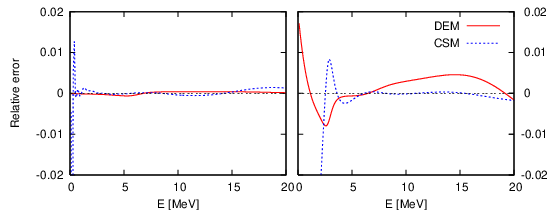
Figure 6 plots the relative error, , of the strength functions calculated with the CSM and DEM models, where stands for the strength function calculated by the Numerov method. Both CSM and DEM reproduce the exact strength very well (within 1 %) over the wide energy range except that the CSM tends to give large errors near the threshold energy. The reason for this is understood from the fact that a correct energy dependence of for close to zero is not manifestly guaranteed in the CSM. The DEM can incorporate such a behavior because it solves the driven equation of motion directly.
4.4 Result with LIT
The same type of bases as in CDA is used to calculate the Lorentz transforms . Since we need in a wide region, the falloff parameters in Eq. (60) are taken in a region wide enough to describe various shapes of the function . To make the inversion from to , it is convenient to express in terms of some plausible functions which the dipole strength of three particles is expected to take. As discussed in Appendix C, should show dependence near , so we assume the following form
| (61) |
which is often employed in the literature [9]. The values calculated as the norm of are fitted from those calculated from the above using Eq. (13). The coefficients are determined by the least squares fitting. The parameter and the maximum number of terms are varied to obtain “converging” as much as possible. Figure 7 compares the two for some values.


Figure 8 displays the corresponding functions. Though the fitting of appears to be very satisfactory except for the case of small , the resulting functions differ from each other, exhibiting some deviations from the exact strength function in the energy region below the peak of the strength. Particularly the strength near the threshold shows an oscillatory behavior and becomes even negative. The latter is unavoidable in general because the expression (61) does not guarantee the positive definiteness. We tested another form
| (62) |
which is always positive. In this case determining the coefficients is not so easy. We used the amoeba routine [25] to search for a minimum of a function. Since it is hard to increase in this routine, no better result was attainable.
5 Conclusion
The electric dipole strength functions provide interesting possibilities of comparisons between theory and experiment. They require accurate theoretical calculations which become very difficult for a three-body system. In recent years, the three-body continuum has started to play a vital role in the study of the excitation mechanism of two-neutron halo nuclei. In the present paper we have developed and compared practical methods to compute dipole strengths for a three-body system with a discretized continuum. Using discrete square-integrable states has the important advantage that powerful techniques developed for bound-state variational studies can be employed such as the versatile expansions in Gaussian states.
The new techniques to compute the strength function with a discrete basis are a direct approach with discrete states (CDA method) and the calculation of a summed expression of the strength function involving a solution of an inhomogeneous driven equation of motion (DEM method). They both make use of Green’s functions. We have compared them with the complex scaling method (CSM) and the Lorentz integral transform (LIT), also making use of a discretized continuum. An apparent advantage of the CSM and LIT is that strength functions can be obtained from states with unphysical asymptotic behaviors, i.e. asymptotically vanishing functions. However, the Green’s function technique leads to physical asymptotics. In the CDA, the correct asymptotic behavior of scattering states is first obtained, allowing a direct calculation of the dipole strength. In the DEM, the solution of the driven equation of motion has a three-body outgoing-wave behavior.
Numerical tests have been performed with an hyperscalar three-body potential in the hyperspherical-harmonics formalism. They have shown that the LIT method is not as mature as the other ones. The problems encountered with the LIT are not due to the discretized continuum but to the difficulty of accurately inverting the obtained transform. Any significant progress in this inversion would improve the present results. All other methods have provided comparable accurate results. The CSM presents however some accuracy problems at very low energies.
The present approaches are promising tools for the study of realistic three-body strength functions with full account of channel couplings. In the three-body continuum, an infinity of open channels occur at each total energy. They correspond to the various ways of how this energy can be shared between the particles. The necessary extensions will also have to deal with Coulomb potentials for which couplings occur even at large distances.
Acknowledgments
We would like to thank S. Aoyama, W. Leidemann and W. Vanroose for useful and enlightening discussions. This work was supported in part by a Grant-in-Aid for Scientific Research (No. 21540261) and also by the Bilateral Joint Research Project between the JSPS (Japan) and the FNRS (Belgium). W. H. is supported by a Grant-in Aid for Scientific Research for Young Scientists (No. 193978) as a JSPS Research Fellow for Young Scientists. This text presents research results of the Belgian program P6/23 on interuniversity attraction poles initiated by the Belgian Federal Science Policy Office.
Appendix A Solution of an inhomogeneous equation with a boundary condition
The aim of this appendix is to solve Eq. (46) together with (38), where and are assumed to vanish for . From Eq. (49), the logarithmic derivative of at is a known constant given by
| (63) |
We thus need to determine in the interval , which we call , with the constraint that its logarithmic derivative at is .
We try to obtain
in an expansion with some
basis sets
| (64) |
with
| (65) |
Here is an auxiliary function introduced to satisfy the condition for the logarithmic derivative at . In fact the logarithmic derivative of at becomes provided that is chosen as
| (66) |
The equation to determine the coefficients reads
| (67) |
where the round brackets indicate that the integration is to be done in :
| (68) |
The amplitude is determined from .
Appendix B Resolvent in complex scaling method
The complex rotation in the CSM is defined by
| (69) |
where is the degree of freedom.
( for a three-body system).
Using
, it is easy to show
that . A key point is that
this complex transformation makes the outgoing wave damp asymptotically.
For a real potential , the Hermitian conjugation
of is ,
where ∗ denotes the complex conjugation.
Note that the eigenfunctions of ,
and
of Eq. (9),
with different labels
and are not orthogonal in general.
Together with Eq. (9), we consider an accompanying eigenvalue problem
| (70) |
with . The solution of this equation is labeled by the same as that of Eq. (9), and we may choose the solution as follows:
| (71) |
We can show that both sets of and are biorthogonal [28], that is,
| (72) |
if the normalization of is chosen to satisfy
| (73) |
To prove Eq. (72), we start from
| (74) |
The left-hand side is reduced to
| (75) |
Thus for , , which, together with Eq. (73), leads to the biorthogonality relation (72).
It follows from the biorthogonality that the resolvent can be expanded as
| (76) |
Substitution of this into Eq. (8) leads to the strength function (11), but and are defined by
| (77) |
These are shown to be identical to those given in Eq. (12). The equality for is trivial from the definition of . For the case of , we only need to show that and are identical within a -independent phase which may be chosen to be unity. This is justified by comparing the normalization condition, , with the trivial normalization condition for , .
Appendix C Analytic form of electric dipole strength function in three-body continuum
The form of as a function of is vital in inverting Eq. (13) which relates to . Its form may be discussed by examining the matrix element . To this end we assume that the continuum state is approximated by the free wave (53). First we consider a case where is close to zero. Since in the present case, the free wave has -dependence for small , that is, the matrix element behaves like . Hence has an dependence near the threshold. Note that this dependence is different from that of a two-body continuum, where the radial part of the free wave normalized on the energy scale is given for the partial wave by
| (78) |
Here is the reduced mass of the two particles. Thus the electric dipole matrix element for small scales as for the -wave.
To know a more general form of , let us assume that the hyperradial part of the ground state is approximated in terms of a combination of Gaussians, , or Exponentials, . The -dependence of the matrix element becomes for the Gaussians, while it is given by for the Exponentials. The strength close to is included in these functional forms. The analytic form of we are looking for is therefore
| (79) |
with for the Gaussian case, or
| (80) |
with for the Exponential case.
Because the actual continuum deviates from the free wave through the interaction among the particles, neither Eq. (79) nor Eq. (80) is exact. However, a suitable choice of the coefficients may simulate accurately. The Lorentz transform is calculated from Eq. (79) or Eq. (80) according to Eq. (13). The coefficients are then determined by least squares fitting to the overlap function , which is in general never trivial particularly when the number of terms is great. It is thus more popular to use non-squared from as in Eq. (61).
References
- [1] B.V. Danilin, I.J. Thompson, J.S. Vaagen, and M.V. Zhukov, Nucl. Phys. A 632 (1998), 383.
- [2] B.V. Danilin, J.S. Vaagen, T. Rogde, S.N. Ershov, I.J. Thompson, and M.V. Zhukov, Phys. Rev. C 73 (2006), 054002.
- [3] E. Garrido, A.S. Jensen, and D.V. Fedorov, Phys. Rev. C 78 (2008), 034004.
- [4] P. Barletta and A. Kievsky, Few-Body Syst. 45 (2009) 25.
- [5] P. Barletta, C. Romeo-Redondo, A. Kievsky, M. Viviani, and E. Garrido, Phys. Rev. Lett. 103 (2009), 090402.
- [6] E. Nielsen, D.V. Fedorov, A.S. Jensen, and E. Garrido, Phys. Rep. 347 (2001), 373.
- [7] P. Descouvemont, E. Tursunov, and D. Baye, Nucl. Phys. A 765 (2006), 370.
- [8] S. Aoyama, T. Myo, K. Katō and K. Ikeda, Prog. Theor. Phys. 116 (2006), 1.
- [9] V.D. Efros, W. Leidemann, G. Orlandini, and N. Barnea, J. Phys. G: Nucl. Part. Phys. 34 (2007), R459.
- [10] D. Baye, P. Capel, P. Descouvemont, and Y. Suzuki, Phys. Rev. C 79 (2009), 024607.
- [11] T. Myo, K. Katō, S. Aoyama, and K. Ikeda, Phys. Rev. C 63 (2001), 054313.
- [12] T. Egami, T. Matsumoto, K. Ogata, and M. Yahiro, Prog. Theor. Phys. 121 (2009), 789.
- [13] Y. Suzuki, W. Horiuchi, and K. Arai, Nucl. Phys. A 823, (2009), 1.
- [14] S. Shlomo and G. Bertsch, Nucl. Phys. A 243 (1975), 507.
- [15] M. Matsuo, Nucl. Phys. A 696 (2001), 371.
- [16] E. Khan, N. Sandulescu, M. Grasso, and N. Van Giai, Phys. Rev. C 66 (2002), 024309.
- [17] M. Pont and R. Shakeshaft, Phys. Rev. A 51 (1995), 494.
- [18] W. Vanroose, D.A. Horner, F. Martín, T.N. Rescigno, and C.W. McCurdy, Phys. Rev. A 74 (2006), 052702.
- [19] C.W. McCurdy and F. Martín, J. Phys. B: At. Mol. Opt. Phys. 37 (2004), 917.
- [20] P.O. Löwdin, in Advances in Quantum Chemistry (Academic Press) 19 (1988), 87.
- [21] A.T. Kruppa, R.G. Lovas, and B. Gyarmati, Phys. Rev. C 37 (1988), 383.
- [22] I.J. Thompson, B.V. Danilin, V.D. Efros, J.S. Vaagen, J.M. Bang, and M.V. Zhukov, Phys. Rev. C 61 (2000), 024318.
- [23] C. Bloch, Nucl. Phys. 4 (1957), 503.
- [24] M. Hesse, J.-M. Sparenberg, F. Van Raemdonck, D. Baye, Nucl. Phys. A 640 (1998), 37.
- [25] W.H. Press, S.A. Teukolsky, W.T. Vetterling, and B.P. Flannery, in Numerical recipes in Fortran 77, (Cambridge University Press, New York, 1992).
- [26] D. Andreasi, W. Leidemann, C. Reiß, and M. Schwamb, Eur. Phys. J. A. 24 (2005), 361.
- [27] W. Leidemann, Few Body Syst. 42 (2008), 139.
- [28] T. Berggren, Nucl. Phys. A 109 (1968), 265.