Quark Condensate and Effective Action from Dyson–Schwinger Equations

Preprint: ITEP-TH-57/09

A. V. Zayakin^1,2 Affiliation: ¹ Department für Physik der Ludwig-Maximillians-Universität München und
Maier-Leibniz-Laboratory, Am Coulombwall 1, 85748 Garching, Germany V. Khandramai³ Affiliation: ¹ Department für Physik der Ludwig-Maximillians-Universität München und
Maier-Leibniz-Laboratory, Am Coulombwall 1, 85748 Garching, Germany J. Rafelski^4,1 Affiliation: ¹ Department für Physik der Ludwig-Maximillians-Universität München und
Maier-Leibniz-Laboratory, Am Coulombwall 1, 85748 Garching, Germany Affiliation: ² ITEP, B.Cheremushkinskaya, 25, 117218, Moscow, Russia Affiliation: ³ ICAS, Gomel State Technical University, Gomel 246746, Belarus Affiliation: ⁴ Department of Physics, University of Arizona, Tucson, Arizona, 85721 USA

December 9, 2009

Abstract

We obtain the QCD quark condensate from consideration of unquenched quark dynamics in Dyson-Schwinger gluon vacuum. We consider the non-local extension of the condensate and determine the quark virtuality. We also obtain the condensate-driven contribution of the non-perturbative QCD to Euler–Heisenberg Lagrangian of QED in external electromagnetic fields.

pacs

12.38.Aw,12.38.Lg,11.15.Tk

I Overview

We describe a method relying on Dyson–Schwinger equations (DSE) for obtaining (non-local) quark condensate and Euler-Heisenberg type effective action with quarks in loops. We develop a self-consistent scheme based on a full set of DSE with dynamical quarks, ghosts and gluons. Our approach is built on methods and prescriptions we adapt from Fischer [1].

Non-local quark condensate was first introduced by Mikhailov and Radyushkin [2], and further developments followed soon after [3, 4]. The gauge invariant NLC is defined by

C(x^{2})\equiv\langle\bar{q}(x)E(x;0)q(0)\rangle,

(1)

where Wilson phase factor is defined as

E(x;0)=\mathop{\mathrm{Pexp}}\left(ie\int_{\mathcal{C}}A_{\mu}(x)dx^{\mu}\right),

(2)

and the contour $\mathcal{C}$ connects points $x$ and $0$ . In this paper we focus our attention on the first terms in powers of $x$ which are independent of the Wilson line contributions. Wilson line terms are in general very important, and such contributions should be evaluated self-consistently [5], which may be done by the Ericson-Semenoff-Szabo-Zarembo (ESSZ) technique used by us in the previous work [6]. It has been shown within the instanton vacuum model [7] that the form of the NLC is nearly independent on possible irregularities of the path, such as a cusp and thus in general the path can be represented by a straight line.

The initial motivation for introducing a NLC came from its influence on hadron phenomenology. For this reason NLC has been decomposed into the local condensates (LC) and the measure of the quark fluctuations in vacuum, known as the quark virtuality (QV). This quantity related to NLC, is defined as

\lambda_{q}^{2}=\frac{\langle\bar{q}D_{\mu}^{2}q\rangle}{\langle\bar{q}q\rangle},

(3)

(here $D_{\mu}$ is the covariant derivative), arising in the standard operator product expansion (OPE) of the NLC as the coefficient in front of the quadratic term:

C(x^{2})=\langle\bar{q}(0)q(0)\rangle\left[1+\frac{x^{2}}{4}\frac{\langle\bar{q}D^{2}q\rangle}{\langle\bar{q}q\rangle}\right].

(4)

Quark virtuality is related to the gluon-quark trilinear (local) condensate

\frac{\langle\bar{q}D^{2}q\rangle}{\langle\bar{q}q\rangle}\sim\langle\bar{q}g\sigma_{\mu\nu}G^{\mu\nu}q\rangle.

(5)

and thus can be counted as an independent vacuum structure parameter, characterizing the non-perturbative QCD vacuum. The standard estimate for $\lambda_{q}^{2}$ by Chernyak and Zhitnitsky [8] is $\lambda_{q}^{2}\approx 0.4\pm 0.1\mathrm{GeV}^{2}$ . There are larger estimates however, e.g. Shuryak suggests [9] $\lambda_{q}^{2}\sim 1.2\mathrm{GeV}^{2}$ . We note that these numerical values for the correlation length are comparable with the typical hadronic scale.

Our effort to relate DSE and NLC is not the first. An attempt to derive self-consistent equations upon condensates was made by Pauchy Hwang [10] in the large- $1/N_{c}$ limit; unfortunately, this was not developed further. Non-local quark condensate has been obtained within the flat-bottom potential approach to Dyson-Schwinger equations, where typical correlation length of $3\mathrm{GeV}^{-1}$ has been obtained [11]. Dyson–Schwinger equations are solved in [12] for quark dynamical mass and wave-function (no gluons or ghosts solved dynamically; gluon propagator mimicked by an Ansatz, rainbow approximation applied to quark equations); using propagators, the quark-quark non-local condensate and the quark-quark-gluon local condensates are calculated, typical correlation length obtained is $0.5\mathrm{GeV}^{-1}$ . Same methods were used in [13], where virtualities $\lambda^{2}_{u,d}=0.7\mathrm{GeV}^{2},\lambda^{2}_{s}=1.6\mathrm{GeV}^{2}$ are reported. These results are confirmed in [14] and completed with gluon virtuality as well $\lambda^{2}_{g}=0.2\alpha_{s}^{-\frac{1}{2}}-1.0\alpha_{s}^{3}\mathrm{GeV}^{2}$ , the latter exhibiting strong scale dependence via coupling constant. Dyson–Schwinger equations were solved in a similar approximation (no dynamical gluons and ghosts) in [15]; however, surprisingly large values of virtualities have been reported: $\lambda^{2}_{u,d}=12\dots 16\mathrm{GeV}^{2},\lambda^{2}_{s}=14\dots 18\mathrm{GeV}^{2}$ . Till now, there has been no self-consistent treatment of the non-local condensates based on DSE with gluons. We consider this to be a disadvantage of the scheme, since quark fluctuations in vacuum are driven by gluons. We will present our result for QV as function of quark mass.

We describe DSE methodology and calculate the propagators in the next section (II), the non-local condensate (NLC) and its response to an external field is studied in section (III). In section (IV) we do the Euler-Heisenberg type effective action for quarks with non-perturbative DSE propagators in external fields and compare our results to the meson based evaluation. We conclude in section (V).

II Dyson–Schwinger Equations

II.1 Formulation of DSE with Quarks

In this section we review the technique of obtaining quark and gluon propagators in a self-consistent way. We use Fisher’s DSE technique described in [1], and we show that the propagators are reproduced by us in the case with quarks as well – we have already reproduced the gluodynamics sector in our previous study [6].

We apply in our work the Newton optimization method, based on the numerical procedure described in [16]. We solve a system for ghost, gluon and quark propagators, as shown in Fig. (1). Propagator dressing is shown by bulbs, and that of vertices – by transparent bulbs.

Refer to caption — Figure 1: Diagrammatic representation of DSE.

We parameterize the gluon propagator in Landau gauge by the form-factor $F$ , defined via relation

\displaystyle D_{\mu\nu}^{F\,ab}(p)=\delta^{ab}\left(g_{\mu\nu}-\frac{p_{\mu}p_{\nu}}{p^{2}}\right)\frac{F(p^{2})}{p^{2}+i\epsilon},

(6)

and the ghost propagator is parameterized by the form-factor $G$

\displaystyle D^{G\,ab}(p)=\frac{\delta^{ab}}{p^{2}+i\epsilon}{G(p^{2})}.

(7)

Quark propagator is defined as

S(p)=\frac{1}{A(p)}\frac{1}{\hbox to0.0pt{$\displaystyle p$\hss}/\,+M(p)}.

(8)

Finding the scalar form-factors $F,G,A,M$ will yield non-perturbative information on the physical quarks and gluons.

DSE for this system can be written in the form:

\displaystyle\left\{\begin{array}[]{l}\displaystyle\frac{1}{G(p^{2})}-\frac{1}{G(\bar{\mu}_{c}^{2})}=-\left(\Sigma(p^{2})-\Sigma(\bar{\mu}_{c}^{2})\right),\\ \\ \displaystyle\frac{1}{F(p^{2})}-\frac{1}{F(\bar{\mu}_{g}^{2})}=-\left(\Pi(p^{2})-\Pi(\bar{\mu}_{g}^{2})\right),\\ \\ \displaystyle\frac{1}{A(x)}=1-\frac{\Pi_{A}(x)}{A(x)}+\Pi_{A}(\bar{\mu}_{g}^{2})\\ \\ \displaystyle M(x)A(x)=M(\bar{\mu}_{g}^{2})+\Pi_{M}(x)-\Pi_{M}(\bar{\mu}_{g}^{2})\end{array}\right.

(9)

Here $\bar{\mu}_{g,c}$ the are points of subtraction, $\bar{\mu}_{c}=0$ , $\bar{\mu}_{g}=\bar{\mu}$ , $\bar{\mu}$ is the limit of the interval $p^{2}\in(0,\bar{\mu}^{2})$ in the momentum space where we solve DSE, coupling $g^{2}$ is meant to be taken at point $\mu$ : $g^{2}(\bar{\mu}^{2})$ . Gluon vacuum polarization is

\Pi(p^{2})=\Pi^{2c}(p^{2})+\Pi^{2g}(p^{2})+\Pi^{2q}(p^{2}),

(10)

contributions of ghosts $\Pi^{2c}(p^{2})$ and gluons $\Pi^{2g}(p^{2})$ being

\begin{array}[]{l}\displaystyle\Pi^{2c}(p^{2})=N_{c}g^{2}\int\frac{d^{d}q}{(2\pi)^{d}}M_{0}(p^{2},q^{2},r^{2})G(q^{2})G(r^{2}),\\ \\ \displaystyle\Pi^{2g}(p^{2})=N_{c}g^{2}\int\frac{d^{d}q}{(2\pi)^{4}}Q_{0}(p^{2},q^{2},r^{2})F(q^{2})F(r^{2}),\end{array}

(11)

ghost self-energy is

\Sigma(p^{2})=N_{c}g^{2}\int K_{0}(p^{2},q^{2},r^{2})G(q^{2})F(r^{2})\frac{d^{d}q}{(2\pi)^{d}}.

(12)

Quark self-energy is conveniently split into functions $\Pi_{A}$ and $\Pi_{M}$ , given below:

\displaystyle\begin{array}[]{l}\displaystyle\Pi_{M}=\frac{1}{3\pi^{3}}\int d^{4}y\left\{\frac{\alpha(z)}{z(y+M^{2}(y))}\frac{G(z)^{-2d-d/\delta}}{F(z)^{d}}\frac{1}{A(y)}\right.\\ \\ \displaystyle\left.\left[\frac{3}{2}\left(A(x)+A(y)\right)M(y)+\frac{1}{2}\left(\Delta A(x,y)M(y)-\right.\right.\right.\\ \left.\left.\left.\displaystyle-\Delta B(x,y)\right)\left(-z+2(x+y)-(x-y)^{2}/z\right)+\right.\right.\\ \\ \displaystyle\left.\left.+\frac{3}{2}(A(x)-A(y))M(y)\Omega(x,y)(x-y)\right]\right\}\end{array}

(13)

and

\begin{array}[]{l}\displaystyle\Pi_{A}=\frac{1}{3\pi^{3}}\int d^{4}y\left\{\frac{\alpha(z)}{xz(y+M^{2}(y))}\frac{G(z)^{-2d-d/\delta}}{F(z)^{d}}\frac{1}{A(y)}\right.\\ \\ \displaystyle\left.\left[\left(-z+\frac{x+y}{2}+\frac{(x-y)^{2}}{2z}\right)\frac{A(x)+A(y)}{2}-\right.\right.\\ \\ \displaystyle\left.\left.-\left(\frac{\Delta A(x,y)}{2}(x+y)+\Delta B(x,y)M(y)\right)\times\right.\right.\\ \left.\left.\times\left(-\frac{z}{2}+(x+y)-\frac{(x-y)^{2}}{2z}\right)+\right.\right.\\ \\ \displaystyle\left.\left.+\frac{3}{2}\left(A(x)-A(y)\right)\Omega(x,y)\left(\frac{x^{2}-y^{2}}{2}-z\frac{x-y}{2}\right)\right]\right\},\end{array}

(14)

yielding the last two equations of (9). Here auxiliary functions $\Delta A,\Delta B,\Omega,\Delta\Omega$ have been introduced:

\begin{array}[]{ccl}\Delta A(x,y)&=&\displaystyle{\frac{A(x)-A(y)}{x-y}},\\[11.38092pt] B(x)&=&M(x)A(x),\\[5.69046pt] \Delta B(x,y)&=&\displaystyle{\frac{B(x)-B(y)}{x-y}},\\[11.38092pt] \Omega(x,y)&=&\displaystyle{\frac{x+y}{(x-y)^{2}+(M^{2}(x)+M^{2}(y))^{2}}}.\end{array}

(15)

The constructions (13), (14), are taken from [1], we have fixed here a typo originally present in Eq. (13). Parameter $d$ is related to the Ansatz for the quark-gluon vertex that is used. There is no unambiguous way of choosing this parameter, since there is no fully consistent way of truncating DSE without violating some of the worthy properties of the original full tower of equations, and we refer the reader to [1] for a comprehensive discussion on that point. Variable $z$ is a logarithmic variable

z=\ln\frac{p^{2}}{\mu^{2}},

(16)

and scale $\mu$ is yet to be defined upon solving DSE from comparing the obtained coupling $\alpha_{DSE}(z)$ to the known values of Particle Data Group coupling $\alpha_{PDG}(p^{2})$ [17] at point $M$ :

\alpha_{DSE}(\ln(M^{2}/\mu^{2}))=\alpha_{PDG}(M^{2}).

(17)

The coupling constant $g^{2}/4\pi\equiv\alpha$ is expressed in terms of $G,F$ solely [18, 19], as vertex is finite in Landau gauge (at one-loop level)

\alpha_{\mathrm{DSE}}(\ln(p^{2}))=\alpha_{\mathrm{DSE}}(\bar{\mu})F(p^{2})G^{2}(p^{2}).

(18)

In our case we shall use varying scale fixing point $M$ so that we can prove that our results are independent of scale fixing point choice within the error margin of our procedure.

The kernels $M_{0},K_{0},Q_{0}$ are well-known in literature, however to make the presentation self-contained we provide them here:

\displaystyle\begin{array}[]{rcl}K_{0}(x,y,\theta)&=&\displaystyle{\frac{y^{2}\sin^{4}(\theta)}{\left(-2\cos(\theta)\sqrt{xy}+x+y\right)^{2}}},\\[17.07182pt] M_{0}(x,y,\theta)&=&\displaystyle{-\frac{y^{2}\sin^{4}(\theta)}{3x\left(-2\cos(\theta)\sqrt{xy}+x+y\right)}},\end{array}

(19)

\displaystyle\begin{array}[]{r}\displaystyle Q_{0}(x,y,\theta)=-\frac{1}{12x\left(-2\cos(\theta)\sqrt{xy}+x+y\right)^{2}}\times\\[17.07182pt] \displaystyle\left\{y\sin^{2}(\theta)\left[2\cos(2\theta)\left(6x^{2}+31xy+6y^{2}\right)-\right.\right.\\[11.38092pt] \displaystyle-12x\cos(3\theta)\sqrt{xy}+xy\cos(4\theta)-48\cos(\theta)\sqrt{xy}(x+y)-\\[11.38092pt] \displaystyle\left.\left.-12y\cos(3\theta)\sqrt{xy}+3x^{2}+27xy+3y^{2}\right]\right\}.\end{array}

(20)

Scalar variables $x=p^{2}$ , $y=q^{2}$ are introduced; variable $\theta$ is defined via $(p-q)^{2}=x+y-2\sqrt{xy}\cos\theta$ . We neglect the effects of non-trivial dressing of the vertices, since these do not essentially back-react the upon the IR structure of the propagators themselves.

To solve the Dyson–Schwinger equations we use the Ansatz [20, 21]:

\begin{array}[]{l}\displaystyle F(z)=\left\{\begin{array}[]{l}\displaystyle\exp\left(\sum^{\bar{n}}_{i}a_{i}T_{i}(z)\right),\,z\in(\ln\epsilon,\ln\bar{\mu}^{2}),\\ \\ \displaystyle F(\bar{\mu})\left(1+\omega\log\frac{p^{2}}{\bar{\mu}^{2}}\right)^{\gamma},z>\ln\bar{\mu}^{2},\\ \\ \displaystyle Az^{2\kappa},z<\ln\epsilon,\end{array}\right.\\ \\ \displaystyle G(z)=\left\{\begin{array}[]{l}\displaystyle\exp\left(\sum^{\bar{n}}_{i}b_{i}T_{i}(z)\right),\,z\in(\ln\epsilon,\ln\bar{\mu}^{2}),\\ \\ \displaystyle G(\sigma)\left(1+\omega\ln\frac{p^{2}}{\bar{\mu}^{2}}\right)^{\delta},z>\ln\bar{\mu}^{2},\\ \\ \displaystyle Bz^{-\kappa},z<\epsilon.\end{array}\right.,\\ \end{array}

(21)

and similar Ansätze for $M(p),A(p)$ . Here $T_{i}$ are Tschebyschev polynomials, $a_{i},b_{i}$ are unknown coefficients yet to be determined from the numerical solution, $\bar{n}$ is the number of polynomials used (mostly $\bar{n}=30$ has been used here, allowing precision of up to $10^{-10}$ for the coefficients), $\delta=-9/44$ , $\gamma=-1-2\delta$ , $\omega=11N_{c}\alpha(\sigma)/(12\pi)$ . The IR scaling $\kappa$ is chosen to be the standard [22, 23]

\kappa=0.59

(22)

for the case of Brown–Pennington truncation with $\zeta=1$ [21] (for discussion of meaning of $\zeta$ see [24]), which is our case ( $\zeta$ already set to its number value everywhere). Following [25], we employ renormalization constant $\mathcal{Z}_{1}$ redefinition, so that no momentum dependence could possibly enter it, that is

\mathcal{Z}_{1}=\frac{G(y)^{(1-a/\delta-2a)}}{F(y)^{(1+a)}}\frac{G(y)^{(1-b/\delta-2b)}}{F(y)^{(1+b)}}.

(23)

Again, following [25] we choose

a=b=3\delta,

(24)

which minimizes its momentum dependence. Renormalization constant $\mathcal{Z}_{1}$ refers to the piece with a ghost loop in vacuum polarization. The equations are solved by using Newton’s method, described for this particular application by Bloch [16]. The results of the solution are propagator form factors $F,G$ , shown in Fig. (2) on the left, the IR behavior of the propagators corresponds to the standard ghost enhancement and gluon suppression. The coupling $\alpha$ obtained from DSE (18) is shown on the right in Fig. (2). We note here that the IR fixed point seen in the Figure is

\alpha(0)\approx 3

(25)

for $N_{c}=3$ , which is consistent with the up-to-date Dyson–Schwinger results reported by other groups [25, 26].

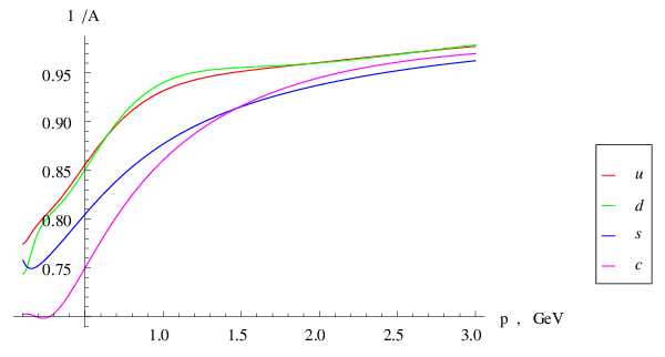
Quark wave-functions were obtained for one quark at a time solving a in a selfconsistent way the DSE, i.e. these are unquenched quarks. They are quite similar to quenched approximation where quark DSE is solved for given glue DSE solution (quenched approximation) The wave function form factors are shown in Fig. (3). Wave-function form factors become perturbatively unity; within an error margin they are no more distinguishable in the UV, although they exhibit different and non-trivial behavior in the IR.

The quark masses are shown in Fig. (4). Physically it is important that UV anomalous dimensions of all the quarks are rendered the same in Fig. (4) , which confirms validity of the procedure. This can be seen from the dashed parallel lines in Fig. (4) In general, in this Section, we confirm all the current knowledge on the DSE with quarks. We improve the numerical convergence by smoothing numerical cut-off on integrals by superposing varying limits, which procedure removes Fourier transform ‘echos’ from the results.

III Non-local Condensate

III.1 Dependence on mass of condensate shape

In this Section we calculate the non-local condensate omitting the Wilson line, study its behavior under external fields and compute the vacuum response due to presence of non-local condensates to external fields.

The nonlocal condensate-related vacuum expectation value (C-VEV)

C_{0}(x)=\langle\bar{\psi}(x)\psi(0)\rangle,

(26)

where local condensate $C(0)$ satisfies $C(0)=C_{0}(0)$ , can be related to propagator as

C_{0}(x)=\frac{1}{(2\pi)^{4}}N_{c}\sum_{i}^{N_{f}}\int d^{4}p\frac{e^{ipx}}{A_{i}(p)}\frac{4M_{i}(p)}{p^{2}+M_{i}^{2}}-(\mbox{PT})

(27)

However, separation the perturbative (PT) part from the non-perturbative propagator is not well-defined. Moreover, some argue that the non-perturbative procedure is producing only the non-perturbative quark propagator and there is no PT subtraction needed. We do not have a good argument to support this reasoning, or, alternatively, a PT part subtraction, thus we follow the former approach. This also does not introduce additional procedure ambiguity. Accordingly, it should be remembered when evaluating our results that the full non-perturbative understanding of QCD vacuum cannot be reached on grounds of Dyson-Schwinger equations alone, without applying additional resummation procedures, e.g. ESSZ-resummation [6]. For this reason our results should be treated as a first qualitative estimate, and not yet as exact predictions.

We think that despite any of the above shortcomings the results we obtain are surprizing. We show the C-VEV in Fig. (5), where we see from top to bottom (at $x\to 0$ ) beginning with the heavy quark $\langle\bar{c}(x)c(0)\rangle$ , $\langle\bar{s}(x)s(0)\rangle$ $\langle\bar{d}(x)d(0)\rangle$ , $\langle\bar{u}(x)u(0)\rangle$ , and last the lightest $u$ quark. Numerical difficulties prevent us from reaching higher mass than $500$ MeV for charm (at scale of 2 GeV). Non-local condensate exhibits some oscillatory behaviour within $2<x<10$ GeV^-1. We believe that these C-VEV oscillations are due to numeric uncertainty, but their persistence and appearance when scale matching of quarks to glue and ghost occurs suggest that further study of this phenomenon is needed, and thus we show these results with C-VEV reaching to 2fm distance. At this large distance the sequence of the C-VEV has reversed with smallest quark mass leading to largest value of C-VEV.

III.2 Local quark condensate and quark virtuality dependence on mass

The standard wisdom [27] about condensate dependence on mass for heavy quarks is

\langle\bar{q}q\rangle=-\frac{1}{12m_{q}}\langle\alpha G^{2}\rangle.

(28)

This relation is usually derived from requiring continuity between heavy and light quarks’ properties, imposed at the scale of about $0.2$ GeV. The behavior of our propagators and wave functions is continuous, yet the dependence on mass we observe is completely different. Another well regarded relation is [28]

\langle\bar{s}s\rangle\sim 0.8\langle\bar{u}u\rangle.

(29)

Note that in our evaluation the local condensate is independent of Wilson line integral and thus our results for $x\to 0$ while still PT subtraction dependent are more secure. For $c$ and $s$ quarks the values one sees in Fig. (5). are considerably larger than expected. Moreover, we find that our condensates increase with mass and does not decrease, as was expected based on above estimates.

The values of condensate is fitted surprisingly well by a simple power law

c(m)=0.2\mathrm{GeV}^{3}\left(\frac{m}{\mbox{1GeV}}\right)^{0.73},

(30)

not at all expected from any qualitative QCD model we know. Mass dependence of condensate is illustrated in Fig. (6). The dashed line is the expected light quark value, the thick line the $c,s$ expectations of Eq.(28). Note that these results are obtained by considering one quark at a time and solving selfconsistently DSE (unquenched single quarks).

It seems that with increasing mass quarks can probe better the non-local glue vacuum fluctuations and thus their response strength increases. The non-locality of glue vacuum structure is usually not considered in the qualitative condensate models. However, there is no argument we can present to align the light quark local condensate as function of $m$ with heavy quark condensate. We also note that when dealing with realistic quarks, their physical magnetic moments must be taken into account. However this effect diminishes with quark mass and cannot explain the heavy quark condensate behavior.

In another attempt to understand this strange behavior, one could suggest that heavy quarks are worse represented by Dyson–Schwinger equations since they tend to decouple and thus one-loop approximation becomes almost free, but at higher loops they might become again important, thus yielding DSE approach invalid. However, this explanation is not valid, since comparison of quenched approximation to the unquenched shows very little difference between the two. Thus the issue of condensate dependence on mass in DSE scheme presented here remains an open question.

Should this behavior be true, this strong dependence on mass of light quark condensate would deeply impact the chiral model analysis of quark masses, where a cornerstone assumption is that light quark condensates have equal value.

Quark virtuality dependence on mass is given in the table 1 below and is shown in Fig. (7). We note the highly regular behavior, following the fit

\lambda^{2}_{q}=0.39{\rm GeV}^{2}\left(\frac{m_{q}}{1{\rm GeV}}\right)^{1.07}

(31)

shows in Fig. (7) For comparison recall that virtualities $\lambda^{2}_{u,d}=0.7\mathrm{GeV}^{2},\lambda^{2}_{s}=1.6\mathrm{GeV}^{2}$ were reported [14], as discussed in Section 1. Recall also $\lambda_{q}^{2}\approx 0.4\pm 0.1\mathrm{GeV}^{2}$ [8] and $\lambda_{q}^{2}\sim 1.2\mathrm{GeV}^{2}$ [9].

III.3 Condensate response to external field

We can also establish the character of condensate dependence on the external field. Considering a diagram Fig. (8),

we derive the $F^{2}$ -order term in the non-local condensate

\langle\bar{\psi}\psi\rangle_{F}=\langle\bar{\psi}\psi\rangle_{0}+F^{2}f_{1}(x)-F_{\nu\alpha}F^{\alpha}_{\mu}\frac{\partial^{2}}{\partial_{\nu}\partial_{\mu}}f_{2}(x),

(32)

where moments $f_{1}$ , $f_{2}$ are

\begin{array}[]{l}\displaystyle f_{1}(x)=\frac{1}{(2\pi)^{4}}\int\frac{e^{ipx}d^{4}p}{A^{3}(p)}\frac{(-8)m(p)}{(p^{2}+m^{2}(p))^{3}},\\ \\ \displaystyle f_{2}(x)=\frac{1}{(2\pi)^{4}}\int\frac{e^{ipx}d^{4}p}{A^{3}(p)}\frac{(-16)m(p)}{(p^{2}+m^{2}(p))^{4}}.\end{array}

(33)

We notice here that not only the character of condensate dependence on $x$ changes due to field switch-on, but it acquires anisotropy. The function $f_{1}$ is shown in Fig. (9). It deserves attention that smallest quark masses bring largest response to field, which is quite reasonable. The resulting parameters are shown in the table (1). It can be seen from analysis of $f_{1}$ that already fields of order of magnitude of $10^{-1}$ GeV² may put the local condensate to zero. This is comparable to the prediction of critical fields for condensate

F_{\rm cr}=\frac{m_{\pi}^{2}}{\log 2}

(34)

by Smilga and Shushpanov [29].

Table 1: Main characteristics of condensate: local amplitude

C(0)

, virtuality

\lambda^{2}

, condensate amplitude variation

\frac{\delta C(0)}{\delta F^{2}}

, virtuality variation

\frac{\delta\lambda_{q}^{2}}{\delta F^{2}}

, infrared exponent

a

(

\langle\bar{\psi}(x)\psi(0)\rangle\sim e^{-ax}

), variation of the infrared exponent

\frac{\delta a}{\delta F^{2}}

. Mass value

m=0.51

in the fourth line is not a misprint against the expected

m=1.27

GeV, but was the largest mass at 2 GeV scale available to us.

\begin{array}[]{|l|l|l|l|l|l|l|l|}\hline\cr m_{q},\mbox{GeV}&q&C(0),\mbox{GeV}&\lambda^{2}_{q},\mbox{GeV}^{2}&\frac{\delta C(0)}{\delta F^{2}},\mbox{GeV}^{-1}&\frac{\delta\lambda_{q}^{2}}{\delta F^{2}},\mbox{GeV}^{-2}&a,\mbox{GeV}&\frac{\delta a}{\delta F^{2}},\mbox{GeV}^{-3}\\ \hline\cr 0.0025&2/3&0.00239&0.00066&0.037&0.00082&0.40&0.20\\ \hline\cr 0.005&1/3&0.0042&0.0013&0.023&0.00094&0.65&0.20\\ \hline\cr 0.105&1/3&0.037&0.039&0.015&0.0017&1.04&0.22\\ \hline\cr 0.51&2/3&0.12&0.18&0.0064&0.0015&1.04&0.37\\ \hline\cr\end{array}

Long-distance correlations will be even more sensitive to fields, since $f_{1}$ decreases slower than condensate itself, thus making pion wave-function a nice candidate for analysis in an external field.

IV Effective Action due to Condensates

One of the simplest nonlinear processes of QED is photon-photon scattering, shown in Fig. (10). In the language of Euler–Heisenberg effective action, the following term is responsible for this kind of processes

\begin{array}[]{l}\mathcal{L}=a(F_{\mu\nu}F^{\mu\nu})^{2}+F_{\mu}^{\nu}F_{\nu}^{\lambda}F_{\lambda}^{\rho}F_{\rho}^{\mu}=\\ \\ =A(F_{\mu\nu}F^{\mu\nu})^{2}+B(F_{\mu\nu}\tilde{F}^{\mu\nu})^{2}.\end{array}

(35)

Coefficients $a,b$ are in case of QED

\begin{array}[]{l}\displaystyle a=-\frac{\alpha^{2}}{36m^{4}},\\ \\ \displaystyle b=\frac{7\alpha^{2}}{90m^{4}},\end{array}

(36)

and $A,B$ are linearly related to them: $A=a+b/2,B=b$ . We shall calculate now these coefficients for condensate contribution of QCD vacuum into QCD-related photon-photon scattering. We shall see at the end that the contribution is larger than expected, compared to standard (perturbative) contribution due to hadrons. However, the magnitude of the effects we find is very small compared to what is experimentally accessible today, and in the foreseeable future, in the domain of intense laser physics.

Strictly speaking, when dealing with realistic quarks, their physical magnetic moments must be taken into account. In the effective action quark magnetic moments would invoke a contribution of the type $\mu_{q}^{4}F^{\mu_{1}\nu_{1}}F^{\mu_{2}\nu_{2}}F^{\mu_{3}\nu_{3}}F^{\mu_{4}\nu_{4}}\mathop{\mathrm{tr}}[\sigma^{\mu_{1}\nu_{1}}\sigma^{\mu_{2}\nu_{2}}\sigma^{\mu_{3}\nu_{3}}\sigma^{\mu_{4}\nu_{4}}]$ . Noting that the outcome might be non-negligible, we leave this contribution aside, since it requires a serious modification of the DSE solution scheme and complicated issues of truncation validity.

To achieve the result we calculate the diagram Fig. (10) with propagators obtained in the previous section, which are responsible for condensates. We do not separate the condensate and the free terms at the level of each propagator, but rather do the full diagram with the full propagators, and then compare to the perturbative terms ( $a,b$ already given above, multiplied by respective quark charges). As momentum dependence of the full diagram on $s,t,u$ invariants would be known only numerically as a result of a calculation, containing numerical data for propagators, we use the following trick. We work out the scattering amplitudes $M(e_{1},e_{2},e_{3},e_{4})$ , given as

\begin{array}[]{l}\tilde{M}_{\mu\nu\lambda\rho}(k_{1},k_{2},k_{3},k_{4})=e^{4}\int\frac{d^{4}p}{(2\pi)^{4}}\mathop{\mathrm{tr}}\left[S(p)\gamma^{\mu}S(p+k_{1})\gamma^{\nu}\right.\\ \\ \displaystyle\left.\hskip 14.22636ptS(p+k_{1}+k_{2})\gamma^{\lambda}S(p+k_{4})\gamma^{\rho}\right].\end{array}

(37)

For the scattering amplitudes at small values of photon frequencies $\omega$ we extract the coefficient at the $\omega^{4}$ term:

\tilde{M}_{\mu\nu\lambda\rho}(k_{1},k_{2},k_{3},k_{4})e_{1}^{\mu}e_{2}^{\nu}e_{3}^{\lambda}e_{4}^{\rho}=M_{0}+\omega^{4}\alpha^{2}M(e_{1},e_{2},e_{3},e_{4}),

(38)

for two specific sets of polarization vectors, namely, $(e_{1\bot},e_{2\bot},e_{3\bot},e_{4\bot})$ and $(e_{1\|},e_{2\|},e_{3\bot},e_{4\bot})$ , ( $e_{i\bot}$ denotes polarization orthogonal to reaction plane, and $e_{1\|}$ polarization in reaction plane), at specific values for $\theta$ (namely, forward scattering $\theta=\pi$ ). These can be expressed as following scalar integrals

\begin{array}[]{l}\displaystyle M(e_{1\bot},e_{2\bot},e_{3\bot},e_{4\bot})=\\ \\ \displaystyle=\int_{0}^{\infty}\frac{32p^{3}dp}{15\left[p^{2}+M(p)^{2}\right]^{8}A(p)^{3}}\left[19p^{8}+75M(p)^{2}p^{6}-\right.\\ \\ \left.-10M(p)^{4}p^{4}-330M(p)^{6}p^{2}+30M(p)^{8}\right]\\ \\ \end{array}

(39)

\begin{array}[]{l}\displaystyle M(e_{1\|},e_{2\|},e_{3\bot},e_{4\bot})=\\ \\ \displaystyle=-\int_{0}^{\infty}\frac{32p^{3}dp}{15\left[p^{2}+M(p)^{2}\right]^{8}A(p)^{3}}\left[7p^{8}-25M(p)^{2}p^{6}-\right.\\ \\ \left.-40M(p)^{4}p^{4}+60M(p)^{6}p^{2}-30M(p)^{8}\right].\end{array}

(40)

Polarization vectors have been

\begin{array}[]{l}e_{\|}=\{0,0,1,0\},\\ e_{\bot}=\{0,0,0,1\},\end{array}

(41)

with center-of-mass kinematics

\begin{array}[]{l}k_{1}=\omega\{1,1,0,0\},\\ k_{2}=\omega\{1,-1,0,0\},\\ k_{3}=\omega\{1,\cos\theta,\sin\theta,0\},\\ k_{4}=\omega\{1,-\cos\theta,-\sin\theta,0\}.\end{array}

(42)

In the expansion we used the fact that $\omega$ is believed to be small, therefore, all non-perturbative momentum-dependent factors ( $M(p),A(p)$ ) are taken at the point $p$ .

On the other hand, the coefficients $M(\dots)$ are known from (35) by direct analysis

\begin{array}[]{l}M(e_{1\bot},e_{2\bot},e_{3\bot},e_{4\bot})=64(2a+b),\\ \\ M(e_{1\|},e_{2\|},e_{3\bot},e_{4\bot})=16(4a+b).\end{array}

(43)

Thus a simple comparison of (39) and (43) yields values for $a,b$ and $A,B$ . They are shown in Table (2).

Table 2: Coefficients

a,b,A,B

of non-linear terms in the effective action. The ‘‘perturbative’’ line shows for comparison the coefficients

a_{0},b_{0},A_{0},B_{0}

for mass

m

in the loops which can be thought of approximately as

\Lambda\sim 300\mathrm{GeV}

; our results are shown as dimensionless ratios against

a_{0},b_{0},A_{0},B_{0}

. Quarks charges

q_{i}=2/3,1/3

are included into coefficients.

\begin{array}[]{|l|l|l|l|l|}\hline\cr&a_{0}&b_{0}&A_{0}&B_{0}\\ \hline\cr PT&-\frac{1}{36m^{4}}&\frac{7}{90m^{4}}&\frac{1}{90m^{4}}&\frac{7}{90m^{4}}\\ \hline\cr\hline\cr{\rm flavor}&a/a_{0}&b/b_{0}&A/A_{0}&B/B_{0}\\ \hline\cr u&0.07732&0.09317&0.1328&0.09317\\ \hline\cr d&0.00302&0.00337&0.00425&0.00337\\ \hline\cr s&0.00019&0.00022&0.0003&0.00022\\ \hline\cr c&0.00064&0.0007&0.00085&0.0007\\ \hline\cr\end{array}

This Table is quite instructive. First of all, the contributions are comparable with the expected hadronic ones. The range of the latter can be estimated roughly within $1/90m_{\pi}^{4}\dots 1/90m_{\rho}^{4}\sim 40\dots 0.05$ GeV^-4. Quarks with large bare masses yield less, as expected on general grounds.

Basing on the analysis of light quark properties we confirm the claims that QCD vacuum cannot be probed via non-linear QED effects until fields of hadron scales $m_{h}^{2}\sim(0.1\mbox{GeV})^{2}$ are reached, actually on scales several times below typical hadronic scale the effect can be felt as contribution to the naive QED estimate of photon-photon scattering.

We believe that the issue of heavy quarks, which have yielded several inconsistencies in the suggested scheme, could be addressed in our scheme once more effort is devoted to understand the solutions of DSE. Moreover, to arrive at realistic results we need to consider schemes with all quarks participating in the solution of DSE equation, and allowing for vertex correction which implements magnetic moment for light quarks.

V Conclusion

Solving one quark-gluon-ghost Dyson-Schwinger equations, we have obtained the quark non-local condensate and quark virtuality as functions of quark mass. The mass dependence of the condensate disagrees with current qualitative wisdom. We could not find an explanation for why this is the case. The growth of the quark condensate with $m^{0.73},m<500\,\mathrm{MeV}$ implies a significant difference between all mass condensates above and beyond any expectations. If confirmed, this result would have considerable impact on hadron phenomenology. For example, the difference in $u$ -quark and $d$ -quark mass and thus implied difference in quark condensate leads to considerable change in chiral analysis of quark masses.

Regarding the influence of an external field on the condensate we predict that fields of order of magnitude of order of magnitude of $10^{-1}$ GeV² can actually destroy local condensate, and even smaller fields can destroy non-local $x$ -dependent condensate at $x\neq 0$ . This result may have direct impact the pion wave function in external fields. As recently shown by Pimikov, Bakulev and Stefanis [30], it is the non-locality of the condensates that is the key point for inclusion of the non-perturbative contributions to the pion form factor. Thus our results on condensates immediately drive the dynamics of pion wave function in external fields.

In addition we predict that light quarks yield important non-perturbative contributions into the photon-photon scattering amplitude, which are comparable with the corresponding perturbative contributions based on loops with light mesons. We stress that this dynamics is essentially condensate-driven, and particularly by its non-locality. Our present non-perturbative evaluation suggests that the critical field, above which the non-linear QCD-QED effects can be seen, is several times lower than the typical hadronic scale. Even so, the experiments to probe the QCD vacuum with intense laser fields are beyond the foreseeable future.

We have outlined in the text an opportunity for further advance which must first focus on the resolution of the mass dependence of quark condensate and better understanding of the related virtuality. The relatively large effects which external fields can impart on the QCD vacuum must be confirmed in the context of such an improved theoretical framework.

Acknowledgments

We thank R.Alkofer, A.Bakulev, S.J.Brodsky, C.Fischer J.Pawlowski, A.Pimikov, M.I.Polikarpov, L. von Smekal for discussions. We are specially grateful to C. Fischer who supplied us with his data on propagators, thus greatly simplifying the tedious process of solving DSE.

AZ thanks F.Gubarev, D.Habs, A.Maas, Yu.M.Makeenko, S.Mikhailov, M.Pak, V.Shevchenko, D.V.Shirkov, V.I.Zakharov, K.Zarembo for in depth discussions on related questions of non-perturbative QCD. AZ also thanks the Organizers of the Tenth Workshop on Non-Perturbative Quantum Chromodynamics at l’Institut Astrophysique de Paris, June 8-12, 2009, for creative scientific atmosphere.

JR thanks Jan Pawlowski for sharing Fish and Chips on the way to the Cairns QCD Topical Workshop which started work on this project. He further thanks Herrn Dietrich Habs for his interest and enthusiastic Bavarian hospitality at the Munich Centre of Advanced Photonics – DFG excellence cluster in Munich.

This work was supported by the DFG Cluster of Excellence MAP (Munich Centre of Advanced Photonics). AZ was in part supported by the RFBR grant 07-01-00526. JR work was supported by a grant from the U.S. Department of Energy DE-FG02-04ER41318.

References

[1] C. S. Fischer (2003), eprint hep-ph/0304233, PhD thesis.
[2] S. V. Mikhailov and A. V. Radyushkin, JETP Lett. 43, 712 (1986).
[3] S. V. Mikhailov and A. V. Radyushkin, Sov. J. Nucl. Phys. 49, 494 (1989).
[4] S. V. Mikhailov and A. V. Radyushkin, Phys. Rev. D45, 1754 (1992).
[5] G. W. Semenoff and K. Zarembo, Nucl. Phys. Proc. Suppl. 108, 106 (2002), eprint hep-th/0202156.
[6] A. V. Zayakin and J. Rafelski, Phys. Rev. D80, 034024 (2009), eprint 0905.2317.
[7] L. A. Trevisan, A. E. Dorokhov, and L. Tomio, Braz. J. Phys. 34, 865 (2004), eprint hep-ph/0405293.
[8] V. L. Chernyak and A. R. Zhitnitsky, Phys. Rept. 112, 173 (1984).
[9] E. V. Shuryak, Nucl. Phys. B328, 85 (1989).
[10] W.-Y. P. Hwang (1997), eprint hep-ph/9702232.
[11] Z.-G. Wang, S.-L. Wan, and K.-L. Wang, Phys. Lett. B498, 195 (2001).
[12] L.-J. Zhou and W.-X. Ma, Chin. Phys. Lett. 20, 2137 (2003).
[13] L.-J. Zhou and W.-X. Ma, Chin. Phys. Lett. 21, 1471 (2004).
[14] L.-J. Zhou, S.-M. Qin, Q. Wu, and W.-X. Ma, Sci. China G51, 1439 (2008).
[15] L.-J. Zhou, L. S. Kisslinger, and W.-x. Ma (2009), eprint 0904.3558.
[16] J. C. R. Bloch, Few Body Syst. 33, 111 (2003), eprint hep-ph/0303125.
[17] C. Amsler et al. (Particle Data Group), Phys. Lett. B667, 1 (2008).
[18] L. von Smekal, R. Alkofer, and A. Hauck, Phys. Rev. Lett. 79, 3591 (1997), eprint hep-ph/9705242.
[19] L. von Smekal, A. Hauck, and R. Alkofer, Ann. Phys. 267, 1 (1998), eprint hep-ph/9707327.
[20] C. S. Fischer, R. Alkofer, and H. Reinhardt, Phys. Rev. D65, 094008 (2002), eprint hep-ph/0202195.
[21] C. S. Fischer and R. Alkofer, Phys. Lett. B536, 177 (2002), eprint hep-ph/0202202.
[22] C. Lerche and L. von Smekal, Phys. Rev. D65, 125006 (2002), eprint hep-ph/0202194.
[23] D. Zwanziger, Phys. Rev. D65, 094039 (2002), eprint hep-th/0109224.
[24] N. Brown and M. R. Pennington, Phys. Rev. D38, 2266 (1988).
[25] R. Alkofer, C. S. Fischer, M. Q. Huber, F. J. Llanes-Estrada, and K. Schwenzer, PoS CONFINEMENT8, 019 (2008), eprint 0812.2896.
[26] M. Q. Huber, R. Alkofer, C. S. Fischer, and K. Schwenzer, Phys. Lett. B659, 434 (2008), eprint 0705.3809.
[27] M. A. Shifman, A. I. Vainshtein, and V. I. Zakharov, Nucl. Phys. B147, 385 (1979).
[28] B. L. Ioffe, Phys. Atom. Nucl. 66, 30 (2003), eprint hep-ph/0207191.
[29] I. A. Shushpanov and A. V. Smilga, Phys. Lett. B402, 351 (1997), eprint hep-ph/9703201.
[30] A. V. Pimikov, A. P. Bakulev, and N. G. Stefanis (2009), eprint 0909.4624.