Transient behavior in systems with time-delayed feedback
Abstract
We investigate the transient times for the onset of control of steady states by time-delayed feedback. The optimization of control by minimising the transient time before control becomes effective is discussed analytically and numerically, and the competing influences of local and global features are elaborated. We derive an algebraic scaling of the transient time and confirm our findings by numerical simulations in dependence on feedback gain and time delay.
keywords
control, time-delayed feedback, transient1 Introduction
Control of nonlinear dynamical systems has attracted much attention since the seminal ground-breaking work of Ott, Grebogi, and Yorke (Ott et al., 1990), and a large variety of different control schemes have been proposed (Fradkov, 2007; Schöll and Schuster, 2008). One particularly successful method called time-delayed feedback control was introduced by Pyragas in order to stabilize periodic orbits embedded in a strange attractor of a chaotic system (Pyragas, 1992). In this scheme, the difference between the current control signal , which is generated from some system variables, and its time-delayed counterpart yields a control force that is fed back to the system. If the time delay matches the period of the target orbit, this control force vanishes. Thus, time-delayed feedback is a noninvasive control method. The Pyragas scheme has been successfully applied for the control of both unstable steady states (Hövel and Schöll, 2005; Dahms et al., 2007) and periodic orbits in different areas of research ranging from mechanical (Blyuss et al., 2008; Sieber et al., 2008) and neurobiological systems (Schöll et al., 2009; Schneider et al., 2009) to optics (Tronciu et al., 2006; Schikora et al., 2006; Flunkert and Schöll, 2007; Dahms et al., 2008) as well as semiconductor devices (Schöll, 2001; Schöll, 2009) and chemical systems (Balanov et al., 2006). On the theoretical part, previous work includes investigations on analytical properties (Just et al., 2004; Amann et al., 2007), asymptotic scaling for large time delays (Yanchuk et al., 2006; Yanchuk and Perlikowski, 2009), and limitations of this powerful control method (Fiedler et al., 2007; Just et al., 2007). However, the transient dynamics of time-delayed feedback control has not been investigated systematically.
In this paper, we aim to obtain a deeper insight into the control mechanism and its efficiency by an analysis of transient times before control is achieved. The transient times and their scaling behavior have been studied in particular in the context of chaotic transients (Tél and Lai, 2008), e.g., in spatially extended systems, where supertransients were found. Here, we consider the case of steady states in linear and nonlinear systems which are subject to time-delayed feedback control. We investigate a generic system beyond a supercritical Hopf bifurcation. Thus, the unstable fixed point can be treated as a linearized normal form above the bifurcation. Furtheron, we focus also on global aspects (von Loewenich et al., 2004; Höhne et al., 2007).
This paper is organized as follows: In Sec. 2, we investigate the transient times of control of an unstable focus in the presence of time-delayed feedback within a linear model and relate this quantity to the eigenvalues of the controlled system. Section 3 is devoted to effects of time-delayed feedback on transient times of fixed point control in a nonlinear system under the influence of stable periodic orbits. We finish with a conclusion in Sec. 4.
2 Linear transients
In this Section, we consider an unstable fixed point of focus type which is subject to time-delayed feedback (Hövel and Schöll, 2005; Dahms et al., 2007). It can be described within a generic model in center-manifold coordinates by a linear system which corresponds to the normal form close to, but above a supercritical Hopf bifurcation whose nonlinear effects will be discussed in Sec. 3. The dynamic equations are given by
| (1a) | |||||
| (1b) | |||||
where corresponds to the regime of unstable fixed point and is the intrinsic frequency of the focus. The control parameters and denote the feedback gain and time delay, respectively. In complex notation , Eqs. (1) become
| (2) |
Similarly, using with amplitude and phase , Eq. (2) can be rewritten in the uncontrolled case () as
| (3) |
The amplitude equation will serve as starting point of our analytical derivations presented later in this Section.
The stability of the system (1) can be inferred from the characteristic equation
| (4) |
where the fixed point is stable if the real part of all eigenvalues is negative. Note that solutions of this transcendental equation can be found analytically using the multi-valued Lambert function which is defined as the inverse function of for (Hövel and Schöll, 2005):
| (5) |
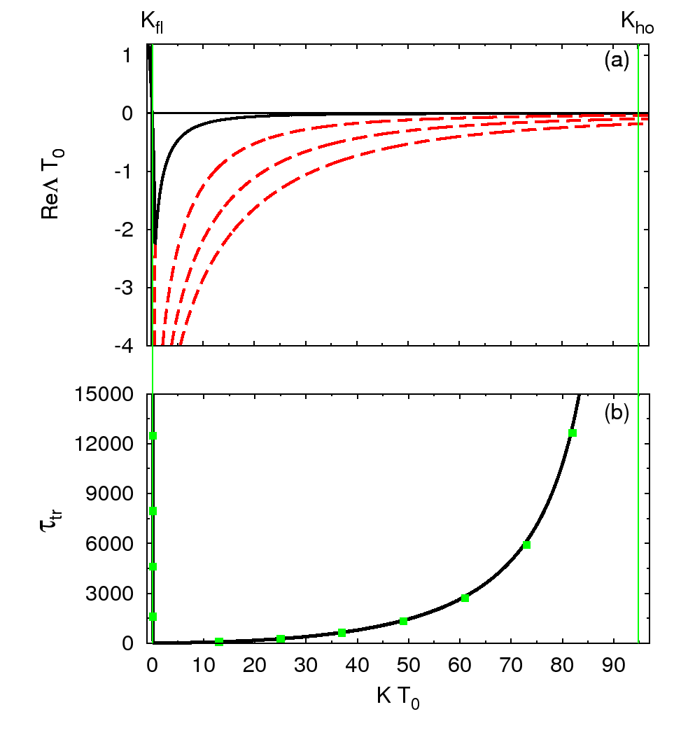
In the following the initial conditions are taken from the uncontrolled system for and the control is switched on at . Figure 1(a) depicts the largest real parts of the eigenvalues calculated from the characteristic equation (4) in dependence on the feedback gain . The time delay is fixed at with the intrinsic timescale . The dashed red curves refer to lower eigenvalues arising from in the limit of vanishing . In the absence of a control force, the system is unstable with . As the feedback gain increases, the largest real part becomes smaller and changes sign at where the system gains stability in a flip bifurcation. Above this change of stability, the largest real part collides with a control-induced branch and forms a complex conjugate pair. For even larger values of , the system becomes unstable again in a Hopf bifurcation at . Both threshold values of are marked as green vertical lines.
In the following, we will derive an analytical relation between the solutions of the characteristic equation and the transient times. Starting from an initial distance , the transient time to reach a neighborhood around the fixed point is given for the uncontrolled case of Eq. (3) by the following expression
| (6) |
Note that corresponds to the real part of the uncontrolled eigenvalue . Time-delayed feedback influences the eigenvalues according to the characteristic equation (4) such that the transient time in the presence of the control scheme becomes
| (7) |
where denotes the largest real part of the eigenvalues which is depicted by the black solid curve in Fig. 1(a).
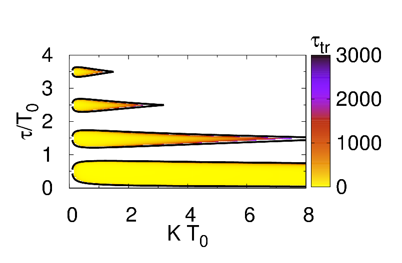
Figure 1(b) displays the transient time in dependence on the feedback gain. The solid curve corresponds to the transient time calculated from Eq. (7). The green dots depict the transient time obtained from numerical simulations of the system’s equation (2), where is measured as the duration to enter a neighborhood of radius starting from an initial distance . One can see that the transient time diverges at the flip bifurcation and the Hopf threshold where the largest real part becomes zero. This is indicated by the solid green lines at and . There is a broad optimum of transient times in a wide range of feedback gain . Thus the efficiency of control is not very sensitive to the choice of , which is not evident from mere inspection of the eigenvalues (Fig. 1(a)).
Figure 2 shows the transient times in the plane parametrized by both control parameters and as color code. Note that there are islands of stability separated by areas for which the control fails to stabilize the fixed point. Similar to Fig. 1(b), the value of the transient time becomes arbitrarily large at the boundary of control. The black solid curves correspond to the boundary of control, i.e., vanishing real part of the largest eigenvalue in Eq. (4). Optimum control, i.e., minimum transient times, occurs in the center of the tongues of stability , .
Since the eigenvalues are given by the Lambert function in Eq. (5), the transient time cannot be written in terms of elementary functions. Nevertheless, an approximation can be given near the values of where the largest real part changes its sign, i.e., at the boundaries of stability. Using a linear approximation of the dependence of on the feedback gain at the flip and Hopf bifurcation points and , one finds for the leading eigenvalue
| (8) |
with . Writing the eigenvalue in terms of the Lambert function as given by Eq. (5) this derivative becomes
| (9a) | ||||
| (9b) | ||||
with the abbreviation . Using the analytical expression for the derivative of (Corless et al., 1996)
| (10) |
for , and using Eq. (5) to express in terms of , it follows from Eq. (9b)
| (11) |
Therefore, for the expression around the flip threshold, where and holds, one obtains
| (12) |
and for the transient time
| (13) |
In analogy, one finds near the Hopf threshold at , where the imaginary part of the largest eigenvalue is given by (Yanchuk et al., 2006), the following expression
| (14) |
which yields
| (15) |
Hence, in both case a power-law scaling of the transient time is obtained.
We note that a supertransient scaling (Tél and Lai, 2008) of the form with positive constants and cannot be found because the derivatives of at do not vanish
| (16) |
as can be seen in Fig. 1(a).

Figure 3 depicts the linear approximations of at the flip and Hopf threshold points and as dashed red lines according to Eqs. (12) and (14), respectively. The insets (b) and (c) display the transient time around these -values as given by Eqs. (13) and (15), respectively. While the linearization yields a good approximation at the flip threshold, its deviations are more pronounced at the Hopf threshold because changes here at a slower rate.
3 Nonlinear transients
This Section is devoted to investigations in nonlinear systems containing periodic orbits. We will consider the Hopf normal form as a generic model given by the following equation (Stuart-Landau oscillator)
| (17) |
As an extension to Eq. (2) of Section 2, a cubic nonlinearity is taken into account with real coefficients and . Before addressing the effects of time-delayed feedback on this system, we will briefly review the uncontrolled case in terms of the transient times. Using again amplitude and phase variables, i.e., , Eq. (17) becomes
| (18a) | |||||
| (18b) | |||||
Note that the equation for the amplitude (18a) yields a periodic orbit with . In the following, we will restrict our consideration to the case which corresponds to a supercritical Hopf bifurcation, i.e., there exists a stable periodic orbit for .
Similar to Sec. 2, the transient time can be calculated from the amplitude equation (18a) as follows
| (19a) | ||||
| (19b) | ||||
where denotes an initial amplitude and the final amplitude is chosen as or for the analysis of the transient time concerning the fixed point at the origin and the periodic orbit, respectively. Note that the coefficients in front of the two logarithmic functions correspond to the inverse of the real part of the eigenvalue of the fixed point and the Floquet exponent of the supercritical periodic orbit, respectively.

Figure 4 depicts the time series of the amplitude and the transient time of the Hopf normal form (17), where panels (a)-(c) and (d)-(f) correspond to a parameter value below () and above () the Hopf bifurcation, respectively. Note that the time series is displayed in linear as well as logarithmic scale.
Below the bifurcation, the stable fixed point at the origin is the only invariant solution. Panel (b) shows that this fixed point is approached exponentially. Panel (c) depicts the transient time in dependence on the initial amplitude according to Eq. (19a). The dashed (red) curve refers to the linear case discussed on Sec. 2 showing the difference to the nonlinear system Eq. (17).
Above the bifurcation (Fig. 4(d)-(f)), the fixed point is unstable and the trajectory approaches the periodic orbit . Note that the dotted (green) and solid curves correspond to initial conditions inside and outside this periodic orbit, respectively. For initial conditions close to the origin the transient time becomes arbitrarily large as the trajectory needs more time to leave the vicinity of the repelling fixed point.
Next, we consider effects of time-delayed feedback control. Applying this control scheme to the Hopf normal form, the system’s equation (17) becomes
| (20) |
with the feedback gain and time delay . In the following, we will keep the time delay fixed at , as in Sec. 2, but set initial conditions as for .

Figure 5 depicts the transient time in dependence on the feedback gain and initial amplitude as color code. The delay time was demonstrated to be an optimal choice in the purely linear system discussed in Sec. 2. The white areas correspond to parameter values for which the trajectory does not reach the fixed point. For the fixed point is unstable. For a certain finite non-zero feedback gain, however, the fixed point can be stabilized by time-delayed feedback. The transient time becomes larger as increases even further until control is lost again similar to Fig. 1(b).
For a better understanding of the success and failure of the time-delayed feedback scheme, Fig. 6 shows the time series for selected combinations of the feedback gain and initial amplitude . Panels (a),(c),(e), and (g) depict the trajectory in the phase space where the arrow indicates the direction. Panels (b),(d),(f), and (h) display the time series of the amplitude . The parameters and are chosen as follows: Figures 6(a)-(d) illustrate the behavior at the left boundary of the yellow region of Fig. 5 with fixed feedback gain . While the fixed point is still stabilized in panels (a),(b) for , the control fails for in panels (c),(d) where a delay-induced stable periodic orbit is asymptotically reached. On the right boundary of Fig. 5 and for fixed , panels (e),(f) correspond again to successful stabilization of the steady state at the origin for , whereas slightly larger feedback gain () of panels (g),(h) results asymptotically in a delay-induced torus (see inset in Fig. 6(h)). This explains the modulation of the stability range in Fig. 5 due to resonances with delay-induced periodic or quasi-periodic orbits which reduce the basin of attraction of the fixed point.


In contrast to the linear case, the controllability displays an interesting non-monotic dependence upon the initial condition , with a strongly reduced range of control at certain values of resembling resonance-like behavior. Although the fixed point is locally stable under time-delayed feedback control in the whole range of shown in Fig. 1(a), the global behavior is strongly modified by a finite size of the basin of attraction. This is reflected in the effect of the initial condition upon the transient time as displayed in Fig. 7 for fixed feedback gain , i.e., along the vertical dotted line indicated in Fig. 5. One can see a strong increase of for small which is followed by a damped oscillatory behavior. For large initial amplitudes, this curve approaches the value corresponding to the uncontrolled system which is added as dashed red curve and calculated from Eq. (19b) for a real part of the eigenvalue of the stabilized fixed point and (fitted parameters). The strong modulation of the transient time with can be explained by the following qualitative argument. It follows from Fig. 2 that control works best in the linear system if where is the intrinsic timescale of the uncontrolled system, and it fails for , . Now, in the nonlinear system, the effective angular velocity changes with distance from the fixed point according to by Eq. (18b). For the angular velocity increases with increasing initial radius . Hence, the period decreases with increasing radius. Thus, for fixed and increasing , the ratio successively passes alternating half-integer and integer values. This suggests that the resonance conditions for best and worst control are alternatingly satisfied, even though the fixed point itself is still linearly stable. By this we can explain the modulation of the transient time in Fig. 7. This is, of course, a simplified argument, since it does not take into account that not only the angular velocity is shifted by the nonlinearity, but also the radial velocity changes nonlinearly with radius by Eq. (18a).

In order to clearly separate the effects of modified angular and radial velocity, we will now consider the limit case where the nonlinearity affects only the angular velocity and hence . Figure 8 illustrates the behavior of for in the -plane. In contrast to Fig. 5, the domain of control is no longer connected but consists of several islands of stability. They are separated by white regions where control fails. The sequence of these white regions with increasing can be qualitatively explained by the condition , , i.e., . Here, the transients do not converge to the fixed point although this is linearly stable, but rather to a delay-induced orbit. This is clear indication of the finite basin of attraction of the fixed point, and of complex global effects in the nonlinear system. Note that our simple qualitative explanation does not describe the exact position of the gaps of stabilization, since changes with increasing time, and the condition holds only for the linear system. Within the stability islands, larger feedback gain leads to longer transients.

Similar to Fig. 7 , Fig. 9 shows a vertical cut of Fig. 8 for fixed feedback gain as indicated by the dotted line. One can see that the transient times becomes arbitrarily large at the boundaries of the stability islands. Note that the transient time is bounded from below by the dashed red curve which corresponds to the uncontrolled case according to Eq. (19b) with and .
4 Conclusion
In conclusion, we have shown that the transient times for control of steady states by time-delayed feedback are strongly influenced by the interplay of local and global effects. In a linear delay system the transient time scales with an inverse power law of the control gain if the boundary of stabilization is approached. In a nonlinear system, e.g., a Hopf normal form, global effects due to coexisting stable delay-induced orbits lead to strongly modulated transient times as a function of the initial distance from the fixed point. These results are relevant for the optimization of time-delayed feedback control.
This work was supported by Deutsche Forschungsgemeinschaft in the framework of Sfb 555.
References
- Amann et al. (2007) Amann, A., Schöll, E., and Just, W. (2007). Physica A, 373, 191.
- Balanov et al. (2006) Balanov, A.G., Beato, V., Janson, N.B., Engel, H., and Schöll, E. (2006). Phys. Rev. E, 74, 016214.
- Blyuss et al. (2008) Blyuss, K.B., Kyrychko, Y.N., Hövel, P., and Schöll, E. (2008). Eur. Phys. J. B, 65, 571–576.
- Corless et al. (1996) Corless, R.M., Gonnet, G.H., Hare, D.E.G., Jeffrey, D.J., and Knuth, D.E. (1996). Adv. Comput. Math, 5, 329.
- Dahms et al. (2007) Dahms, T., Hövel, P., and Schöll, E. (2007). Phys. Rev. E, 76(5), 056201.
- Dahms et al. (2008) Dahms, T., Hövel, P., and Schöll, E. (2008). Phys. Rev. E, 78(5), 056213.
- Fiedler et al. (2007) Fiedler, B., Flunkert, V., Georgi, M., Hövel, P., and Schöll, E. (2007). Phys. Rev. Lett., 98, 114101.
- Flunkert and Schöll (2007) Flunkert, V. and Schöll, E. (2007). Phys. Rev. E, 76, 066202.
- Fradkov (2007) Fradkov, A.L. (2007). Cybernetical Physics: From Control of Chaos to Quantum Control. Springer, Heidelberg, Germany.
- Höhne et al. (2007) Höhne, K., Shirahama, H., Choe, C.U., Benner, H., Pyragas, K., and Just, W. (2007). Phys. Rev. Lett., 98(21), 214102.
- Hövel and Schöll (2005) Hövel, P. and Schöll, E. (2005). Phys. Rev. E, 72, 046203.
- Just et al. (2004) Just, W., Benner, H., and v. Löwenich, C. (2004). Physica D, 199, 33.
- Just et al. (2007) Just, W., Fiedler, B., Flunkert, V., Georgi, M., Hövel, P., and Schöll, E. (2007). Phys. Rev. E, 76(2), 026210.
- Ott et al. (1990) Ott, E., Grebogi, C., and Yorke, J.A. (1990). Phys. Rev. Lett., 64, 1196.
- Pyragas (1992) Pyragas, K. (1992). Phys. Lett. A, 170, 421.
- Schikora et al. (2006) Schikora, S., Hövel, P., Wünsche, H.J., Schöll, E., and Henneberger, F. (2006). Phys. Rev. Lett., 97, 213902.
- Schneider et al. (2009) Schneider, F.M., Schöll, E., and Dahlem, M.A. (2009). Chaos, 19, 015110.
- Schöll (2001) Schöll, E. (2001). Nonlinear spatio-temporal dynamics and chaos in semiconductors. Cambridge University Press, Cambridge.
- Schöll (2009) Schöll, E. (2009). Pattern formation and time-delayed feedback control at the nano-scale. In G. Radons, B. Rumpf, and H.G. Schuster (eds.), Nonlinear Dynamics of Nanosystems. Wiley-VCH, Weinheim.
- Schöll et al. (2009) Schöll, E., Hiller, G., Hövel, P., and Dahlem, M.A. (2009). Phil. Trans. R. Soc. A, 367, 1079–1096.
- Schöll and Schuster (2008) Schöll, E. and Schuster, H.G. (eds.) (2008). Handbook of Chaos Control. Wiley-VCH, Weinheim. Second completely revised and enlarged edition.
- Sieber et al. (2008) Sieber, J., Gonzalez-Buelga, A., Neild, S., Wagg, D., and Krauskopf, B. (2008). Phys. Rev. Lett., 100(24), 244101.
- Tél and Lai (2008) Tél, T. and Lai, Y.C. (2008). Phys. Rep., 460(6), 245.
- Tronciu et al. (2006) Tronciu, V.Z., Wünsche, H.J., Wolfrum, M., and Radziunas, M. (2006). Phys. Rev. E, 73, 046205.
- von Loewenich et al. (2004) von Loewenich, C., Benner, H., and Just, W. (2004). Phys. Rev. Lett., 93(17), 174101–174101–4.
- Yanchuk and Perlikowski (2009) Yanchuk, S. and Perlikowski, P. (2009). Phys. Rev. E, 79(4), 046221.
- Yanchuk et al. (2006) Yanchuk, S., Wolfrum, M., Hövel, P., and Schöll, E. (2006). Phys. Rev. E, 74, 026201.