Specific heat of the simple-cubic Ising model
Abstract
We provide an expression quantitatively describing the specific heat of the Ising model on the simple-cubic lattice in the critical region. This expression is based on finite-size scaling of numerical results obtained by means of a Monte Carlo method. It agrees satisfactorily with series expansions and with a set of experimental results. Our results include a determination of the universal amplitude ratio of the specific-heat divergences at both sides of the critical point.
pacs
05.50.+q, 64.60.Cn, 02.60.-xI introduction
Though real magnetic systems were supposed to be Heisenberg-like, the Ising model was originally introduced [1] as a simplified model of magnetic ordering, because its relative simplicity offers better possibilities for a theoretical analysis. In later years, it was found, however, that Ising-like magnetic systems do exist. This is because real systems consist of spins embedded in a crystal lattice, and the resulting anisotropy field due to the neighboring charges may lift the O(3) symmetry of an unperturbed spin. Depending on the character of the perturbation, the spin may have an ‘easy axis’ or an ‘easy plane’. Here we consider the former case, which leads to Ising-like behavior.
In many cases, the perturbation is relatively small and the system will approximately behave Heisenberg-like, except near an ordering transition where the paramagnetic state transforms into a long-range ordered one. Near the transition, crossover [2, 3, 4] occurs to Ising-like behavior. The critical singularities are then described by the Ising set of critical exponents. In some other cases, the perturbation due to the crystal field is so strong that the magnetic spins assume a true Ising character. This situation occurs when the ionic angular momentum is described by a spin quantum number , and the crystal field lifts the degeneracy of the eigenstates such that the doublet is lowest in energy, with the higher levels so far away that they play no role, even in the presence of exchange interactions between neighboring spins. Then the low-lying doublet can be described by an effective spin-1/2 Ising Hamiltonian. This situation is known to occur for the Co2+ ion in a tetrahedral coordination. It occurs also for some rare-earth ions like Dy3+ and Yb3+ in a sufficiently strong crystal field, with the provision that here the magnetic moments are due to spin as well as orbital angular momentum, and should thus be denoted instead of .
If such ions are embedded in a crystal structure for which theoretical predictions for the thermodynamical properties such as the specific heat exist, comparison with experiments may be possible [5, 6]. Such comparisons were made for dysprosium phosphate [7, 6] and for some alkali cobalt halides [8, 9]. These systems were found to behave, at least approximately, as the Ising models on the diamond lattice and the simple-cubic lattice respectively.
The best way to obtain theoretical results for the thermodynamic properties of these models would obviously be an exact solution, but this is known to be a very difficult problem. It is thus noteworthy that it was claimed recently by Zhang [10] that a conjectured exact solution was found for the three-dimensional Ising model. However, Perk [11] and Wu et al. [12] pointed out that Zhang’s result for the free energy and the underlying arguments are flawed. Here it may be added that Zhang’s result for the critical point of the simple-cubic Ising models is not compatible with independent and mutually consistent numerical estimates [13, 14]. The difference with Zhang’s result exceeds the estimated numerical accuracies [13, 14] by several orders of magnitude.
In the absence of an exact solution, one may still resort to approximations. At temperatures sufficiently far above and below the critical point, excellent approximations exist in the form of series expansion of the partition function or the free energy, such as given in Refs. 15 and 16 for the model on the simple-cubic lattice. In the critical region, the series of a finite length become inaccurate, and a method to extrapolate these series on the basis of a critical scaling assumption, such as used by Butera and Comi [17], is needed. In the case of Rb3CoCl5 (rubidium cobalt chloride) [9] the required theoretical prediction for the specific heat near criticality was also obtained this way. A similar analysis has been performed for the specific heat of DyPO4 (dysprosium phosphate) [7, 6], which was instead compared with series expansions for the diamond lattice. However, these specific-heat analyses were conducted at a time that the value of the critical exponent was not well known, for instance, was set to zero in Ref. 9. Moreover, Wegner’s correction to scaling [18] was not included.
In order to obtain accurate predictions for the heat capacity in the critical region, one may apply Monte Carlo simulations. Cluster simulation methods [19, 20], which strongly reduce critical slowing down, allow statistically accurate simulations in the critical region. Extrapolation of the finite-size simulation data to the thermodynamic limit is possible if the simulations cover a range of finite sizes exceeding the correlation length. Whereas this still excludes, as a result of the divergence of the correlation length, a narrow temperature range about the critical point, one may attempt to describe the extrapolated data by means of a scaling formula. The present work reports our efforts along this line for the case of the energy and the specific heat of the Ising model on the simple-cubic lattice.
In Sec. II we describe our Monte Carlo simulations, and the extrapolation to infinite system size. The derivation of scaling formulas for the energy and the specific heat, and the data analysis in terms of these formulas, are presented in Sec. III. Section IV discusses the numerical accuracies, provides comparisons with results from series expansions and with a set of experimental results, and ends with a few concluding remarks.
II Numerical technique
The reduced Hamiltonian (Hamiltonian divided by ) of the Ising model is denoted
| (1) |
where the indices and label nearest-neighbor lattice sites on the simple-cubic lattice. The sum is on all nearest-neighbor pairs, and the spins can assume values . The coupling is defined by where is minus the energy of a pair of parallel nearest-neighbor spins, the Boltzmann constant, and the temperature. The canonical reduced free energy density is equal to
| (2) |
where is the partition function, the number of spins, and the sum is on all spin configurations . The energy and the specific heat per particle, as expressed in dimensionless units, follow from the derivatives of to :
| (3) |
II.1 Monte Carlo calculations
Substitution of Eqs. (2) and (1) in Eqs. (3) leads to
| (4) |
and
| (5) |
where the ensemble averages , which are defined as
| (6) |
can be sampled directly using importance sampling.
The simulations involved the sampling of the energy, as well as its square, for Ising systems on simple-cubic lattices, with periodic boundary conditions. The system sizes were chosen as powers of 2 in the range , and in addition as and 12. About samples were taken for , for , for , and for . Each sample was preceded by a number or Wolff cluster steps and/or Metropolis sweeps, depending on the value of in comparison with the critical coupling [14]. For , Wolff clusters tend to be very small and only Metropolis sweeps were applied, and for only Wolff cluster steps. In the intermediate range, a few Metropolis sweeps were supplemented with a number of Wolff cluster steps. The number of Wolff clusters was chosen roughly equal to the inverse of the relative Wolff cluster size. The coupling was given some 50 different values chosen to cover a wide range about the critical point.
II.2 Extrapolation
The analysis of the numerical finite-size data was done on the basis of well-documented finite-size scaling methods [21]. For non-critical systems with sizes exceeding the correlation length, the data for the energy should approximately behave as
| (7) |
from which the extrapolated energy was obtained by means of a least-squares analysis. A small-system-size cutoff was applied when necessary to obtain a satisfactory residual . This cutoff varied between far away from the critical point, and at a distance from the critical point. No reliable extrapolations were obtained for less than a few times , with the exception of , where one expects that the finite-size-dependent energy converges as a power of , which again enables extrapolation to . Typical estimated accuracies of the extrapolated results for are in the order of .
The same extrapolation procedure was applied to the finite-size data for the specific heat with . Typical accuracies of the extrapolated results for are estimated as at most a few times for and , up to a few times in the vicinity . The extrapolated data are listed in the Appendix.
III Scaling and least-squares analysis
III.1 Derivation from renormalization theory
The analysis of the extrapolated data was done on the basis of scaling as derived from renormalization theory. The relevant equations follow from the assumptions that the picture described in the following paragraph is valid.
The free energy density of the infinite system, expressed as a function of thermodynamic parameters (), can be written as the sum of an analytic part and a singular part . The singular part can be written as a function of Wegner’s [22] nonlinear scaling fields , which are analytic functions of the in a neighborhood of a critical point under investigation. Thus
| (8) |
The singular part satisfies the scaling equation as implied by the renormalization theory. A rescaling of the linear dimensions by a factor thus leads to
| (9) |
where is the dimensionality and the are the renormalization exponents associated with the scaling fields , with the temperature exponent positive, and the other exponents negative. The choice thus yields
| (10) |
where has the sign of . Furthermore, is an analytic function in a neighborhood of the , , , .
On the basis of this set of assumptions, we may Taylor expand the free energy in powers of the arguments and , and then expand the ’s in the ’s, resulting in an expression depending only on the physical temperature fields, but with expansion coefficients that remain to be determined. We follow this procedure, restricting number of scaling fields in the expansion of Eq. (10) to two, namely the temperature field and the irrelevant field . The corresponding exponents are denoted and respectively. The temperature exponent determines the leading singularity in the temperature-induced ordering transition, while the irrelevant exponent generates Wegner’s correction to scaling [18]. Expansion of the right-hand side of Eq. (10) thus yields
| (11) |
where is the th derivative of to its second argument. The scaling fields are expanded as analytic power series in the temperature-like parameter , defined by
| (12) |
The analytic part of the free energy can be expanded directly in powers of . The resulting expansion of the total free energy density in powers of and can be expressed in , the only variable physical temperature parameter in our problem, as given by the Hamiltonian (1). Differentiation of the resulting expansion of the free energy density to yields the dimensionless energy . For dimensions, the leading terms are included in
| (13) |
where we have included the first three terms in the sum on in Eq. (11), and is an analytic function of related to by
| (14) |
The dimensionless specific heat of the model (1) satisfies
| (15) |
and its expansion thus follows by differentiation of the energy, Eq. (13). This leads to
| (16) |
The parameters and , and their derivatives as they appear in Eqs. (13) and (16), are expanded in powers of as
| (17) |
where stands for the sign of , for its opposite, and
| (18) |
The scales of and are determined by setting .
III.2 Fits
Whereas Eq. (11) includes, in principle, infinitely many terms, for numerical work it is necessary to truncate the expansion of , as well as those of and the scaling fields, at a finite order. Expression (13) for the energy already contains the implicit simplification that there is only one irrelevant field, and that the expansion of is truncated at second order. Moreover, higher orders in the expansion of the temperature derivative of the irrelevant field were neglected. We shall reconsider these simplifications in Sec. IV.1. No further simplifications were made in the derivation of Eq. (16) from Eq. (13).
Many attempts were made to fit Eqs. (13) and (16) to the numerical data, using different ranges of , and different sets of parameters as determined by the orders at which the expansions were truncated. The unknown parameters in each set were determined by means of a Levenberg-Marquardt nonlinear least-squares analysis. Since Eqs. (13) and (16) depend on the same parameters, the data for the energy and the heat capacity were simultaneously fitted by one set of parameters.
A fit was considered satisfactory if it met three criteria: first, the residual has to be compatible with the number of degrees of freedom; second, there should be sufficiently large ranges of overlap with the accurate predictions from the low- and high-temperature series expansions; and third, at least the amplitudes of the leading terms in the fit formulas should be reasonably stable under variations of the -interval and of the number of correction terms in the temperature field and the analytic background. In Table 1 we list the smallest satisfactory set of parameters thus obtained. We skipped the ellipses in Eqs. (13) and (16), and included terms up to order in the expansion of , up to in that of , and up to in the analytic parts expressed by the first sums in Eqs. (13) and (16). The residual of this fit was , to be compared with the number of degrees of freedom . Since possible correlations between specific heat and energy data could influence the estimation of the errors in the fitted parameters, we have analyzed the correlations between the deviations of the energy and of the specific heat with respect to the fit formula. We find a correlation coefficient of -0.066 which is not significant, and does not provide a reason to reconsider our error estimates.
| parameter | value | error margin |
|---|---|---|
| fixed | ||
| 0.06 | ||
| 0.09 | ||
| —— | ||
| fixed | ||
| 0.6 | ||
| 0.016 | ||
| 0.012 | ||
| 0.2 | ||
| 0.4 | ||
| 0.4 | ||
| 0.8 | ||
| 0.000004 | ||
| 0.8 | ||
| 12 | ||
| 50 | ||
| 100 | ||
| —— | ||
| fixed | ||
| fixed | ||
| fixed |
During the least-squares analysis, we found that some parameter values changed significantly when the -interval and/or the numbers of parameters in the expansions of and of the analytic background were varied. Such shifts were sometimes comparable to the error margins as estimated from statistics based on the accuracy of the Monte Carlo results. This applied in particular to those of the and the with . In this respect the amplitudes , , , and, to some extent, and were better behaved. The error estimates listed in Table 1 take into account the variation of the parameter values between these fits.
IV Discussion
IV.1 Choice of parameters and their error margins
Equation (11) and the fits of and use only one irrelevant field, while, according to Newman and Riedel [23], corrections to scaling could also arise from a second irrelevant field with exponent . We note that corrections generated in first order of would thus, in the present context, be practically indistinguishable from those generated in second order by . For this reason, we have not included a separate term containing . Furthermore, the energy, Eq. (13), neglects a contribution due to the possible -dependence of the irrelevant field. Such a term behaves as and is thus a factor smaller than the leading correction. The third-order correction in , which is also neglected, has nearly the same exponent.
Another correction that was neglected is one with an integer exponent , associated with the discreteness of the cubic lattice. The presence of such corrections could modify the higher-order correction amplitudes given in Table 1, but the criterion did not yield indications that a term with should be included.
Some insight in the relative importance of the corrections due to different orders of the irrelevant field can be obtained by comparing the fit including the second order of , as given in Table 1, to fits including up to the first order. Reasonable fits, as following from the criterion, could only be be obtained by including three more coefficients or . Moreover, these coefficients tended to assume much larger values. For this reason, we prefer the fit up to second order in , although the fit up to first order also yields a satisfactory numerical representation of the critical energy and specific heat.
Only the parameters , , and , describing the leading few orders of and , were about the same for both types of fits. It is thus clear that not too much physical significance should be given to the subleading and higher-order parameters given in Table 1, except that they provide a numerical description of and in the critical region.
The relative errors in the amplitudes and of the second order term in , as given in Table 1, are appreciable, and far exceed those of the first-order amplitudes and . For this reason we believe that it is not necessary to include a third-order correction, or other terms with approximately the same exponent.
IV.2 Comparison with existing results
IV.2.1 Series expansions
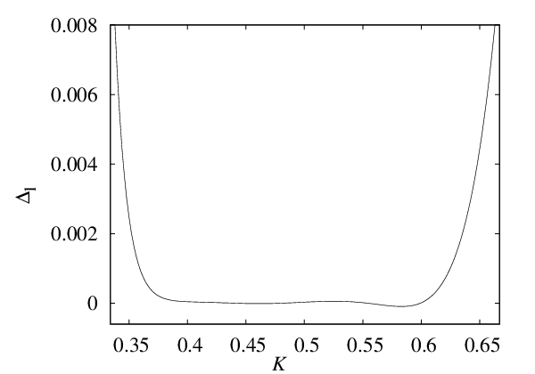
Numerical evaluation of Eq. (16) allows comparison with results from series expansions. The low-temperature series for the energy is provided by Bhanot et al. [15] up to order 25 in . The specific heat, as obtained by differentiation of this series, is in good agreement with Eq. (16) in the interval . The differences, which are shown in Fig. 1, do not exceed . For , outside the range of the least-squares fit, our representation of the specific heat with Eq. (16) is no longer accurate and the differences increase sharply. The increasing differences for are due to the truncation of the low-temperature series to 25 terms.
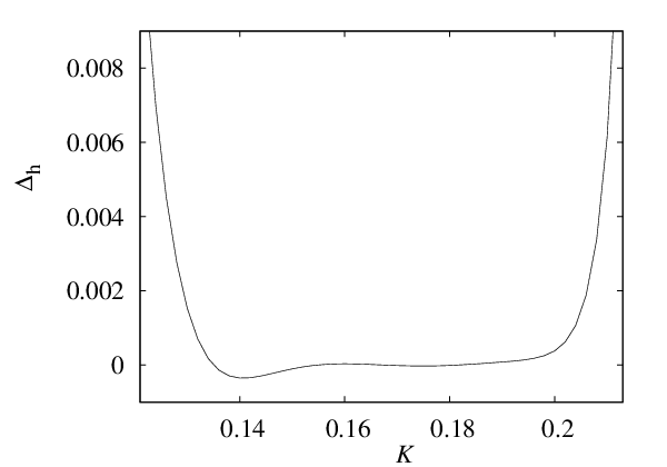
For temperatures above the critical point, a comparison can be made based on the series expansion up to order 46 of the free energy as provided by Arisue and Fujiwara [16], with the help of Eq. (3). The differences with Eq. (16) are less than interval , as plotted in Fig. 2. For , outside the range of the fit, Eq. (16) rapidly loses its accuracy. The increasing differences for are due to the truncation of the series.
IV.2.2 Amplitude ratios and analytic background
The fit up to first order in yielded a universal amplitude ratio , which is to be compared to the result of the fit including the second order of , which is as follows from the parameter values in Table 1. Based on the consistency between these two results, we believe that the latter result is reliable. This result is close to an estimate 0.541 (14) by Bagnuls et al. [24] from field theory, and to the result 0.523 (9) obtained by Liu and Fisher [25] based on series expansions, and slightly smaller than 0.560 (10) as determined from Monte Carlo data by Hasenbusch and Pinn [26].
Another universal ratio that can be constructed from the results in Table 1 concerns the corrections-to-scaling amplitudes. The data in the table suggest , which differs considerably from as obtained by Bagnuls et al. [24] (note the sign difference with respect to the notation used by Bagnuls et al., which is related to the factor in our Eq. (16)). The sign of this amplitude ratio is in agreement with the conclusions of Liu and Fisher [27].
As noted in Sec. IV.1, there may be corrections to scaling governed by an irrelevant field with exponent , and thus indistinguishable from contributions in second order of . It is thus possible that the amplitudes and as given in Table 1 contain contributions due to the field . Therefore, the resulting ratio may not qualify as a universal amplitude ratio.
Our result for the critical energy, , can be compared with results obtained from series analysis. It is slightly smaller than the result obtained by Sykes et al. [28], slightly larger than found by Liu and Fisher [25], and in agreement with found by Butera and Comi [29]. Our result is also consistent with the Monte Carlo estimates due to Jensen and Mouritsen [30], and due to Hasenbusch and Pinn [26].
IV.2.3 Comparison with experimental results for Rb3CoCl5
As implied in the Introduction, the magnetic Co2+ ions in rubidium cobalt chloride assume a spin-1/2 Ising character. This has been experimentally confirmed [31] in the related compound Cs3CoCl5. The magnetic moments are aligned along the direction of the tetragonal crystal structure. The Co2+ ions are arranged in a simple Bravais lattice, with equivalent positions [32]. Furthermore, electron-spin resonance results [33] for Cs3CoCl5 showed that the exchange interaction with the two nearest neighbors in the crystallographic direction has the same magnitude as that with the four nearest neighbors in the plane, so that one may expect that the theoretical results for the simple-cubic Ising model are applicable. Specific-heat and magnetic susceptibility measurements [9] on Rb3CoCl5 showed that a phase transition to an antiferromagnetic phase occurs at K. It was indeed found that the specific heat (which does not depend on the sign of ) did agree with the theoretical predictions available at that time. These predictions were based on series expansions due to Baker [34] and Sykes [35], and on the assumption that the specific-heat exponent . In view of later results for the specific-heat exponent, as well as the effect of Wegner’s correction [18], the comparison made in Ref. 9 may thus not be considered as entirely satisfactory. In Fig. 3 we show the experimental data together with Eq. (16), as well as results from the low- and high-temperature series. This comparison with the experimental data, which involves only one adjustable parameter, the critical temperature, shows that the specific heat of Rb3CoCl5 agrees reasonably well with the predictions for the simple-cubic Ising model. The data in Fig. 3 suggest small deviations at low as well as at high temperatures, but there the specific heat becomes very small, so that the experimental error margins, which include the uncertainty of heat capacity of the empty apparatus, become appreciable. A comparison of the experimental data listed in Ref. 9 with the results from Eq. (16) show that deviations up to a few percent occur also in the range . But these deviations do not display an obvious systematical trend, and may possibly be attributed to the fact that the measured heat capacity is, near criticality, the result of integration of a highly nonlinear function over a nonzero temperature range.
It thus seems that new experiments on Rb3CoCl5 are needed to firmly establish deviations with respect to the predictions for the simple-cubic Ising model. Such deviations would be a logical consequence of the tetragonal symmetry of Rb3CoCl5, which implies that there is no reason why the coupling in the -direction should be precisely equal to that in the direction. Also the presence of interactions with further neighbor spins, which include small magnetic dipole-dipole interactions, should lead to deviations.

IV.3 Conclusion
The formula Eq. (16), supplemented by Eqs. (17), (18), and (12) and by the parameter values in Table 1, describes the specific heat of the three-dimensional Ising model in the interval . Comparisons with low- and high-temperature series expansions yield satisfactory agreement in the intervals and respectively. The differences between Eq. (16) and the results from series expansions are at most in the mentioned intervals. These differences are smaller than the statistical errors in the Monte Carlo results on which Table 1 is based, as may be expected since the number of 100 data points far exceeds the number of 16 free parameters in the fit formula, so that in effect averaging occurs. Since Eq. (16) continues to satisfactorily describe the extrapolated Monte Carlo data until a distance from the critical point, we conclude that the error margin in Eq. (16) does not exceed that of the Monte Carlo data, i.e., it will be limited to at most a few times at . Larger uncertainties are expected for because of the error margins in the critical amplitudes, exponents and temperature. Taking into account these numerical uncertainties, Eq. (16) can be used in the interval for comparison with experiments on systems that are described by the simple-cubic Ising Hamiltonian.
In addition, our results show that Monte Carlo simulations can be used to determine the universal leading amplitude ratios and even the nonasymptotic ratio . Thus far, the correction amplitudes have been studied by means of series analysis, field theory, and crossover scaling, see e.g., Refs. 27, 24, 36, 37.
Acknowledgements.
HB thanks J.M.J. van Leeuwen for valuable discussions, and the Lorentz Fund (The Netherlands) for financial support.References
- [1] E. Ising, Z. Physik 31, 253 (1925).
- [2] M. Suzuki, Phys. Lett. A 35, 23 (1971); M. Suzuki and F. Tanaka, Prog. Theor. Phys. 3, 1085 (1973).
- [3] M. E. Fisher and P. Pfeuty, Phys. Rev. B 6, 1889 (1972).
- [4] F. J. Wegner, Phys. Rev. B 6, 1891 (1972).
- [5] L. J. de Jongh and A. R. Miedema, Adv. Phys. 23, 1 (1974).
- [6] W. P. Wolf, Braz. J. of Phys. [online] 30, n. 4, 794 (2000).
- [7] J. C. Wright, H. W. Moos, J. H. Colwell, B. W. Magnum and D. D. Thornton, Phys. Rev. B 3, 843 (1971).
- [8] R. F. Wielinga, H. W. J. Blöte, J. A. Roest and W. J. Huiskamp, Physica (Amsterdam) 34 223 (1967).
- [9] H. W. J. Blöte and W. J. Huiskamp, Phys. Lett. A 29, 304 (1969).
- [10] Z.-D. Zhang, Phil. Mag. 87, 5309 (2008).
- [11] J. H. H. Perk, arXiv:0811.1802.v2 (2008).
- [12] F. Y. Wu, B. M. McCoy, M. E. Fisher and L. Chayes, Phil. Mag. 88, 3093 (2008).
- [13] P. Butera and M. Comi, Phys. Rev. B 62, 14837 (2004).
- [14] Y. Deng and H. W. J. Blöte, Phys. Rev. E 68, 036125 (2003), and references therein.
- [15] G. Bhanot, M. Creutz and J. Lacki, Phys. Rev. Lett. 69, 1841 (1992); G. Bhanot, M. Creutz, U. Glassner and K. Schilling, Phys. Rev. B 49, 12909 (1994).
- [16] H. Arisue and T. Fujiwara, Phys. Rev. E 67, 066109 (2003). There is a typo in the 42th order term; the correct value appears in hep-lat/0209002 (2002).
- [17] P. Butera and M. Comi, Phys. Rev. B 69, 174416 (2004).
- [18] F. J. Wegner, Phys. Rev. B 5, 4529 (1972).
- [19] R. H. Swendsen and J. S. Wang, Phys. Rev. Lett. 58, 86 (1987).
- [20] U. Wolff, Phys. Rev. Lett. 62, 361 (1989).
- [21] For reviews, see e.g. M. P. Nightingale in Finite-Size Scaling and Numerical Simulation of Statistical Systems, ed. V. Privman (World Scientific, Singapore 1990), and M. N. Barber in Phase Transitions and Critical Phenomena, eds. C. Domb and J. L. Lebowitz (Academic, New York 1983), Vol. 8.
- [22] F. J. Wegner, in Phase Transitions and Critical Phenomena, eds. C. Domb and M. S. Green (Academic, N.Y. 1976), Vol. 6.
- [23] K. E. Newman and E. K. Riedel, Phys. Rev. B bf 30, 6615 (1984).
- [24] C. Bagnuls, C. Bervillier, D. I. Meiron and B. G. Nickel, Phys. Rev. B 35, 3585 (1987).
- [25] A. J. Liu and M. E. Fisher, Physica A (Amsterdam) 156, 35 (1989).
- [26] M. Hasenbusch and A. Pinn, J. Phys. A 31, 6157 (1998).
- [27] A. Liu and M. E. Fisher, J. Stat. Phys. 58, 431 (1990).
- [28] M. F. Sykes, D. L. Hunter, D. S. McKenzie and B. R. Heap, J. Phys. A 5, 667 (1972).
- [29] P. Butera and M. Comi, Phys. Rev. B 60, 6749 (1999).
- [30] S. J. K. Jensen and O. G. Mouritsen, J. Phys. A 15, 2631 (1982).
- [31] H. G. Beljers, P. F. Bongers, R. P. van Stapele and H. Zijlstra, Phys. Letters 12, 81 (1964).
- [32] H. M. Powell and A. F. Wells, J. Chem. Soc. 359 (1935).
- [33] R. P. van Stapele, J. C. M. Henning, G. E. G. Hardeman and P. F. Bongers, Phys. Rev. 150, 310 (1966).
- [34] J. M. Baker. Phys. Rev. 129, 99 (1963).
- [35] M. F. Sykes, private communication cited in Ref. 9.
- [36] R. Schloms and V. Dohm, Phys. Rev. B 42, 6142 (1990).
- [37] M. A. Anisimov, S. B. Kiselev, J. V. Sengers and S. Tang, Physica A (Amsterdam) 188, 487 (1992).
Appendix: Extrapolated energy and specific heat
| error | error | ||||
|---|---|---|---|---|---|
| 0.12 | 0.382236 | 0.000020 | 0.13 | 0.419100 | 0.000109 |
| 0.14 | 0.457696 | 0.000007 | 0.15 | 0.498271 | 0.000098 |
| 0.16 | 0.541261 | 0.000008 | 0.166 | 0.568535 | 0.000448 |
| 0.17 | 0.587433 | 0.000007 | 0.172 | 0.597108 | 0.000047 |
| 0.178 | 0.627251 | 0.000049 | 0.18 | 0.637719 | 0.000009 |
| 0.184 | 0.659300 | 0.000052 | 0.19 | 0.693640 | 0.000008 |
| 0.195 | 0.724504 | 0.000007 | 0.196 | 0.730987 | 0.000060 |
| 0.2 | 0.757945 | 0.000005 | 0.202 | 0.77224 | 0.000011 |
| 0.205 | 0.794807 | 0.000016 | 0.21 | 0.836533 | 0.000053 |
| 0.213 | 0.865007 | 0.002836 | 0.22165460 | 0.990604 | 0.000004 |
| 0.224 | 1.135886 | 0.000083 | 0.225 | 1.184077 | 0.000113 |
| 0.226 | 1.228851 | 0.002835 | 0.227 | 1.270902 | 0.001567 |
| 0.228 | 1.310761 | 0.000069 | 0.229 | 1.348806 | 0.000084 |
| 0.23 | 1.385036 | 0.000010 | 0.232 | 1.453408 | 0.000128 |
| 0.235 | 1.547095 | 0.000082 | 0.24 | 1.684411 | 0.000006 |
| 0.25 | 1.908377 | 0.000006 | 0.26 | 2.084422 | 0.000011 |
| 0.268 | 2.200165 | 0.000117 | 0.27 | 2.226207 | 0.000025 |
| 0.28 | 2.342331 | 0.000013 | 0.29 | 2.438392 | 0.000020 |
| 0.3 | 2.518570 | 0.000013 | 0.31 | 2.585908 | 0.000017 |
| 0.32 | 2.643039 | 0.000137 | 0.33 | 2.691193 | 0.000121 |
| 0.34 | 2.732442 | 0.000779 | 0.35 | 2.767639 | 0.000008 |
| 0.36 | 2.797886 | 0.000224 | 0.37 | 2.823926 | 0.000119 |
| 0.38 | 2.846340 | 0.000055 | 0.39 | 2.865798 | 0.000070 |
| 0.4 | 2.882622 | 0.000005 | 0.42 | 2.909917 | 0.000030 |
| 0.44 | 2.930623 | 0.000034 | 0.45 | 2.939050 | 0.000003 |
| 0.46 | 2.946380 | 0.000022 | 0.48 | 2.958427 | 0.000035 |
| 0.5 | 2.967777 | 0.000002 | 0.6 | 2.990703 | 0.000001 |
| 0.65 | 2.994958 | 0.000001 | 0.7 | 2.997255 | 0.000001 |
| error | error | ||||
|---|---|---|---|---|---|
| 0.12 | 0.05212 | 0.00004 | 0.14 | 0.07736 | 0.00005 |
| 0.15 | 0.09382 | 0.00013 | 0.16 | 0.11381 | 0.00004 |
| 0.166 | 0.12812 | 0.00008 | 0.17 | 0.13882 | 0.00005 |
| 0.172 | 0.14458 | 0.00010 | 0.178 | 0.16391 | 0.00012 |
| 0.18 | 0.17094 | 0.00012 | 0.19 | 0.21445 | 0.00035 |
| 0.195 | 0.24361 | 0.00031 | 0.2 | 0.27950 | 0.00110 |
| 0.205 | 0.32850 | 0.00093 | 0.208 | 0.36500 | 0.00100 |
| 0.21 | 0.39573 | 0.00114 | 0.214 | 0.48216 | 0.00165 |
| 0.215 | 0.51335 | 0.00261 | 0.216 | 0.54767 | 0.00157 |
| 0.217 | 0.58500 | 0.00200 | 0.227 | 2.11009 | 0.00675 |
| 0.228 | 2.01738 | 0.00323 | 0.229 | 1.95000 | 0.01000 |
| 0.23 | 1.87829 | 0.00300 | 0.232 | 1.76800 | 0.00150 |
| 0.235 | 1.64500 | 0.01000 | 0.238 | 1.52800 | 0.00300 |
| 0.24 | 1.46600 | 0.00200 | 0.25 | 1.23138 | 0.00041 |
| 0.26 | 1.06294 | 0.00031 | 0.27 | 0.93268 | 0.00200 |
| 0.28 | 0.82520 | 0.00060 | 0.29 | 0.73597 | 0.00094 |
| 0.3 | 0.66021 | 0.00072 | 0.31 | 0.59383 | 0.00085 |
| 0.35 | 0.39923 | 0.00039 | 0.36 | 0.36325 | 0.00036 |
| 0.37 | 0.33045 | 0.00024 | 0.38 | 0.30110 | 0.00020 |
| 0.39 | 0.27460 | 0.00020 | 0.4 | 0.25058 | 0.00025 |
| 0.42 | 0.20890 | 0.00020 | 0.44 | 0.17428 | 0.00013 |
| 0.45 | 0.15910 | 0.00020 | 0.46 | 0.14567 | 0.00012 |
| 0.48 | 0.12158 | 0.00010 | 0.5 | 0.10160 | 0.00010 |
| 0.55 | 0.06470 | 0.00015 | 0.6 | 0.04109 | 0.00010 |
| 0.65 | 0.02593 | 0.00008 | 0.7 | 0.01632 | 0.00004 |