Delays in Open String Field Theory
Abstract:
We study the dynamics of light-like tachyon condensation in a linear dilaton background using level-truncated open string field theory. The equations of motion are found to be delay differential equations. This observation allows us to employ well-established mathematical methods that we briefly review. At level zero, the equation of motion is of the so-called retarded type and a solution can be found very efficiently, even in the far light-cone future. At levels higher than zero however, the equations are not of the retarded type. We show that this implies the existence of exponentially growing modes in the non-perturbative vacuum, possibly rendering light-like rolling unstable. However, a brute force calculation using exponential series suggests that for the particular initial condition of the tachyon sitting in the false vacuum in the infinite light-cone past, the rolling is unaffected by the unstable modes and still converges to the non-perturbative vacuum, in agreement with the solution of Hellerman and Schnabl. Finally, we show that the growing modes introduce non-locality mixing present with future, and we are led to conjecture that in the infinite level limit, the non-locality in a light-like linear dilaton background is a discrete version of the smearing non-locality found in covariant open string field theory in flat space.
Keywords:
String Field Theory, Tachyon Condensation, Light-like Tachyon Rolling, Delay Differential Equations1 Introduction
While the free action of open string field theory [1] is local in the sense that it involves not more than two derivatives of the string field, it is well known that the interaction term of Witten’s string field theory [2] contains infinitely many derivatives. Theories with more than two, but finitely many, derivatives [3, 4] suffer either from an unbounded Hamiltonian or from ghosts11 1 See, however, [5] for an example of quantization of a theory with four derivatives, with no ghost and bounded (but non-hermitian) Hamiltonian., but these instabilities do not necessarily survive in the limit of infinitely many derivatives. Perhaps the simplest way to see this is that the propagator in a theory with finitely many derivatives is the inverse of a polynomial and therefore has poles, some of them ghosts. In the limit of infinite number of derivatives, however, the propagator becomes the inverse of a function that might have only one zero, corresponding to a regular excitation. It might even have no zero at all, like in -adic string theory where the propagator is an exponential (furthermore, this exponential propagator renders all loop diagrams finite [6]).
In cubic open string field theory, the form of the nonlocality is universal, the higher derivatives of any field always appearing in the interaction as
| (1) |
where , and we use the signature . In this case one can see the nonlocality explicitly because is a smearing of as can be seen from the convolution formula [7]
| (2) |
For a homogeneous time-dependent problem, one would take as the fundamental field and write , which can then be written as a convolution as in Eq. (2). A consequence is that the equation of motion of a homogeneous time-dependent string field involves the string field not only at time but at all times, both in the past and in the future of . One can treat this kind of equation either as a convolution equation using Eq. (2), or as a differential equation of infinite order. It must be understood, however, that such a differential equation cannot be seen as a limit of finite-order differential equation; in particular the initial value problem becomes different when we have infinitely many derivatives (see [8] for a rigorous discussion, and [9] which contains some similar results).
A time-dependent equation of motion with infinitely many derivatives which is of particular physical interest, is the equation describing the decay of an unstable D-brane. A well-known problem is that, on the one hand, a boundary conformal field theory (BCFT) analysis shows that one should expect a monotonic decay of the tachyon down its potential [10] and that the energy of the D-brane is converted into very massive closed strings at rest, behaving like dust [11] (tachyon matter). On the other hand, numerical solutions of string field theory [12, 13] show a completely different behavior. Namely, the tachyon does reach the non-perturbative vacuum, but it then continues further and starts oscillating around it with diverging amplitude. Although the tachyon can climb arbitrarily high up the potential, the energy conservation is not violated because the kinetic energy can be negative. In fact, it may seem that energy conservation obviously discards a monotonically rolling tachyon that would stop at the local minimum of its potential. However, this is not totally trivial because one could imagine that the energy of the D-brane is somehow stored in the very high-order derivatives of the tachyon, still allowing for a monotonic rolling. But this is actually ruled out [14, 15] because one can write the expression of the energy in an integral form which makes it clear that, in fact, a monotonically rolling tachyon cannot conserve energy. It is now believed that these ever-growing oscillations are not catastrophic after all. For one thing the string field is not a gauge-invariant observable; but more concretely, it was shown in [16], that a field redefinition mapping the cubic SFT action to the boundary SFT action, would also map the oscillating solution to a well-behaved solution. More recently, it was shown [17] that the closed string boundary state obtained from the rolling tachyon solution, coincides with the BCFT boundary state.
It is interesting to investigate how this wild rolling changes if we somehow couple the closed strings sector to the open string SFT action. The most consistent way to do this would be to consider open-closed string field theory [18]; but solving the equations of motion of the purely closed sector [19] involves a much higher level of difficulty [20, 21, 22, 23, 24, 25, 26, 27, 28]. A somewhat more manageable approach would be to consider a fixed closed string background, but the SFT action becomes in general non-polynomial in a generic closed background [29], hence also hard to solve. What can be done, however, is to minimally couple gravity to the open SFT action. It has been shown, for instance, that minimally coupling an open superstring tachyon to a FRW metric tames the wild oscillations of the tachyon; and convergent rolling tachyon solutions were found numerically [15]. In [30], which was the motivation for the present work, Hellerman and Schnabl considered open SFT in a linear dilaton background. They chose a light-like dilaton gradient and a string field depending only on the light-cone time . This is physically motivated because a bubble of true vacuum is expected to expand at the speed of light [31]. If the radius of the bubble is large enough, we can focus on one small patch and approximate it by a plane, and we choose the light-light coordinate (which we call light-cone time) to be orthogonal to this plane. Moreover, with this ansatz important simplifications occur. In particular, using the fact that is an exactly marginal operator, Hellerman and Schnabl were able to use the results of [32, 33] in order to prove that the rolling tachyon asymptotes to the tachyon vacuum [34] at large light-cone time. On a more explicit footing, Hellerman and Schnabl also considered the SFT action truncated at level zero in Siegel gauge (i.e. keeping only the tachyon). Here the light-cone simplification manifests itself by changing the nature of the non-locality. The non-locality of Eq. (1), which by virtue of Eq. (2), involves the tachyon field at all times, becomes simply the tachyon at some retarded light-cone time . The equation of motion for the tachyon is then
| (3) |
A numerical solution to this equation was worked out by Hellerman and Schnabl. Their method, however, didn’t allow them to go very far in light-cone time, but enough to see convincingly that the tachyon reaches the vacuum after oscillating around it with a decreasing amplitude. In [35], Barnaby et al. considered the initial value problem and the stability of light-like rolling in -adic string theory and in SFT at level zero. In particular, they were able to numerically solve Eq. (3) for a much larger light-cone time interval. Their numerical method is based on the diffusion equation [36, 37, 38]. Although this method can in principle be generalized to higher levels, it is hard to do so in practice.
The motivation for our present paper, was to investigate further the light-cone rolling in Siegel gauge by considering higher-level fields. We will consider levels , , and , where the notation means that we are keeping fields up to level and interactions up to total level . Our results are three-fold.
Firstly, we realized that equations of the type (3) are known in the mathematics literature as delay differential equations (abbreviated DDEs). The most widely used method for numerically solving DDEs is the method of steps. Using this method, we show that solving Eq. (3) numerically becomes surprisingly easy. Moreover, the generalisation to higher levels is straightforward.
Secondly, we show that when we include higher-level fields, the nice picture of the string field gently oscillating around the vacuum with decreasing amplitude, takes a serious hit. Indeed, we show that already at level two, the tensor fields which must be included in our analysis, bring derivatives into the equations of motion in such a way that these become a so called system of higher order neutral DDEs with one positive delay. Such DDEs cannot in general be solved with the method of steps. We have to do some simplifications before obtaining numerical solutions. What we can do, however, is to look at the equations of motion close to the vacuum. We will find that the latter effectively contain several delays. This would pose no further conceptual difficulty if all delays were positive, but we show that we obtain negative delays as well. In other words, the equations of motion effectively involve the fields at some past light-cone times, but also at some future light-cone times. We show that if we have both negative and positive delays, there exist growing oscillation modes around the vacuum. This suggests that the string field may not converge to the non-perturbative vacuum. This seems to be in contradiction with the analytic solution obtained in [30], and also with our numerical solution obtained by expanding the fields in exponential series (this provides in principle a very accurate solution but only up to a limited light-cone time). But the two pictures can be reconciled if we notice that the initial conditions for the analytic solution (which are the same as those for the exponential series solution) are very special. The diverging modes might not be excited for this particular solution, but our results imply that a small change in the initial conditions can render the rolling non-convergent.
Thirdly, by studying the equations of motion near the vacuum at level four, we show that there are more delays at this levels, and that they are more spread, both towards the past and towards the future. We are led to conjecture that in the large level limit, one recovers a discrete version of the non-locality (1). Subsequently setting the dilaton gradient to zero, the delays become less and less spaced, and we will recover (1). We conclude that in particular, the nice simplification of the non-locality that happens at level zero, is only accidental.
This paper is structured as follows: In the next section, we calculate the action and derive the equations of motion at level two. We give a short review of DDEs in Appendix A and the complete results are given in Appendices B and C. We solve the level-zero equation with the method of steps, and we attempt to do the same at level two. We show what problems we face and what can be done to get some information on the rolling at this level. In Section 3, we study the linearized equations of motion near the vacuum. We show that negative delays appear at level two and four and conclude the general form of non-locality in the linear dilaton background. In order to do so, we need to calculate the determinants of polynomial matrices. A naive approach fails if the matrices are too large, so we explain a little-known method for calculating such determinants in Appendix D. In Section 4, we discuss further the consequences of our results. And at last, we offer a review of linear dilaton CFT in Appendix E.
2 Light-like dynamics of the vacuum transition in Siegel gauge
This section is divided into several paragraphs. At first we show how to derive the equations of motion of open string field theory in a linear dilaton background with level truncation. We present more details of the calculation, on the one hand to introduce the notation, and on the other hand because they are omitted too often. After that we briefly describe how we solved the resulting delay differential equations on the computer. To that end we explain how astonishingly natural it is in our setup to choose the infinitely many initial conditions required for producing a unique solution. We test our machinery in the simplest possible case of level zero, and observe excellent agreement with the literature [30, 35]. We then go beyond level zero and explain our results at level two and four, which can be summarized as follows: The individual modes of the string field are initially in the perturbative vacuum, then, driven by the tachyon, they grow steeply. Finally they oscillate around their respective vacuum expectation values with decaying amplitudes.
Derivation
If we write the string field in terms of vertex operators as , the action of Witten’s open string field theory reads
| (4) |
where the functions are the conformal transformations mapping each string (semi-disk) to the common interaction upper-half plane.
We have derived the action and equations of motion with two independent methods. First we calculated the action by hand, calculating explicitly the conformal transformations , and then the CFT correlators 22 2 For a detailed derivation of the correlator in the linear dilaton background, cf. [39].33 3 Note that we use the complex derivative instead of the real derivative. :
| (5) | |||||
The new objects serve as a tool to quickly work out the combinatorics of the contractions - just expand the product into a polynomial in and observe the following rules:
- 1.
Replace
- 2.
Contract products of two s using
- 3.
Remove all terms with an odd number of s.
- 4.
Note that the general expression diverges if . For correlators of normal ordered products (e.g. ) these terms precisely cancel, providing a non-singular result. In this case we can further simplify with the additional rule
Remove all terms in with and all -products at the same point, .
The dilaton background enters explicitly in two ways:
- 1.
the delta function is updated to include the breaking of the translation invariance by the linear dilaton background
where the delta function of a complex argument is formally defined by the following integral representation
(6) - 2.
through the modified conformal transformation law
needed when mapping the string field vertices to the interaction worldsheet.
In order to make sure that our results are correct, we redid the same calculation with the method of conservation laws. Luckily, the conservation laws for an anomalous vector (like in a linear dilaton background) were already worked out by Rastelli and Zwiebach in [40]. This method has the advantage of being easy to implement on a computer. In our case we wrote a mathematica program. To our satisfaction both methods agreed entirely. Since the calculations become rather cumbersome at higher levels to do by hand, we relied on our code for the equations of motion at levels (2,6) and (4,8).
Explaining our notation we will quickly see that at level two, the string field written out in its mode expansion can be reduced to just eight spacetime fields. We follow the conventions by [41] (except that we call their ) and write the string truncated to level two fields. Working in the Siegel gauge, we can eliminate those terms containing a -ghost mode, and due to the twist symmetry of the action, we can consistently set all terms at odd levels to zero. This leaves us with the following expression for the string field at level two:
| (7) |
Since we work in spacetime dimensions, expr. (7) contains 379 spacetime fields. But in the case of light-like tachyon rolling, we can drastically reduce the number of fields needed in our calculation. Working in the light-cone frame we can split the dimensions into light-like and ordinary components
We assume the linear dilaton gradient light-like, . By rotational symmetry we can choose a coordinate system where . Furthermore we consider spacetime fields in expr. (7) that depend only on the first lightcone coordinate . As detailed in appendix B, we can then focus on the following eight (of 379) fields to compute the action:
| (8) |
Note that is the tachyon field and is the scalar field associated with the contribution of to the trace of by
| (9) |
The resulting action is presented in appendix B, both in Lorentz covariant form and explicitly using (8). To check its correctness, one can take the limit of vanishing dilaton gradient, and compare to the action found in [41]. Both expressions agree as desired.
With the action computed, we can proceed to deriving the equations of motion in notationally compact manner. For a Lagrangian containing arbitrary orders of field derivatives , the Euler-Lagrange equation is
In this notation the derivatives are not symmetrized, their order matters:
This is just a matter of more convenient bookkeeping as we sum over all combinations of indices. In a compact notation we can define the differential operator which returns the equation of motion for the field when applied to the Lagrangian depending on and possibly other fields to any order in the field derivatives:
Let’s see how to apply this in a concrete example, take a generic interaction term from , e.g. and compute its contribution to the equation of motion. When deriving the equation of motion for the tachyon field we apply . We use because is independent of the -coordinate. Fields with a tilde are defined by
Now derive the equation of motion:
Applying to the whole term, it becomes apparent that it acts essentially as a translation operator when :
where finally the tilde was eliminated because . The translation operator simply shifts the argument by . This is a generic feature in every interaction term, we therefore define the symbol
for the shifted point to abbreviate the notation. The reason for introducing is that it simplifies the calculation significantly. As an example, consider the chain rule
The set of eight equations of motion contains derivatives of up to fourth order, each equation is quite lengthy with one notable exception: the equation of motion for is short and can be solved easily:
The equation is linear in , hence we set to obtain a solution. As a matter of fact this still admits non-trivial solutions for the other seven fields. This observation was also made in [42], in the related context of OSFT using the lightcone basis for the modes of the string field. This is a peculiarity of level (2,4). Indeed, already at level (2,6) one cannot consistently set to zero anymore.
Setting to zero at level (2,4) reduces the length of the equations of motion by about one third and the total differential order from 21 to 17. The resulting set of equations of motion is presented in appendix C. The seven equations contain a total of 144 terms. For reference we list the seven remaining fields
| (10) |
Let , denote one of the above fields, e.g. is the tachyon field. Then the generic form of an equation of motion is 44 4 To simplify the notation, we set .:
| (11) |
The first two terms come from the kinetic term in the action. They have the same sign except for the tachyon and are evaluated at position . All derivatives are understood with respect to . All terms in the sum arise from the cubic interaction. They are evaluated at and contain derivatives of up to the third order. In fact many of the real-valued coefficients are zero.
Solving the Equations of Motion
Given the general structure of the equations of motion (11), let us now focus on solving them at level . There are derivatives with respect to at both points: (max: 1st order) and (max: 3rd order). The total differential order of the system of equations is 17. Because of the non-locality (fields at and at ) these are not ordinary differential equations (ODEs). It is the key observation that, mathematically speaking, we have a system of coupled delay differential equations of the neutral type (NDDE) with one constant delay . The theory of delay differential equations (DDE) has been developed to great extent in the 20th century as this type of differential equation arises in a large array of disciplines: populations dynamics, machine control theory, neutron diffusion, spreading of diseases, retarded propagation in classical electrodynamics etc. We give a short introduction to DDEs, highlighting the differences to ODEs, in appendix A. Further useful references are [43, 44, 45].
In order to solve DDEs we use the method of steps, explained further in Appendix A. The basic idea is to reduce the problem of computing the solution over a full interval to subintervals where the DDE reduces to an ODE which is solved with standard methods. In order to obtain a unique solution, it is however not sufficient to give an initial condition at one point as in the ODE case: initial conditions over a finite interval (of the length of the delay ) have to be specified. These conditions are called the initial data. They are essentially uniquely determined when we require that the tachyon condensation starts in the perturbative vacuum.
There are other methods. For instance Barnaby et al. [35] transformed the level-zero DDE into an equivalent diffusion-like local partial differential equation problem with suitable boundary conditions, solved that with standard codes and finally transformed back to obtain the DDE solution. For the system of equations at level (2,4), their method seems cumbersome to apply. In contrast, the method of steps is powerful enough to easily extend to the case of several unknowns. For more details on diffusion methods, we refer the reader to
We have seven coupled equations for seven fields with derivatives up to the third order. The numerical stability and convergence properties of the method of steps have been studied carefully in the past decades, cf. [45] for an extensive review of numerical methods. The problem can now be considered a standard one, much like solving a system of ODEs numerically. This implies that the user has to carefully check the consistency of the numerical solution, preferably by independent methods. Much of the effort in this section is aimed in that direction.
On the computer we need dimensionless numbers. As of now we work in units where . For convenience we choose .
Choosing initial data
Let us now see how to supply initial data for each field to obtain a unique solution to the equations of motion. A priori we could choose any initial data, but physical reasons nearly completely fix them. Consider as an example the tachyon field . In principle we would like to obtain the solution from the equations of motion. On the computer we can only obtain a solution on some finite interval . We then need to fix the tachyon on , with the delay . To find constraints recall that we are interested in the tachyon condensation solution: the solution should initially be in the perturbative vacuum (string field ) and in the end arrive at the non-perturbative vacuum. Hence at sufficiently small the absolute value of the tachyon and all other six fields from (10) should be small
As we take we can neglect all interaction terms in the equations of motion (11) and receive dramatically simplified equations. In other words, we linearize the equations of motion around zero, , and neglect all terms quadratic in the small quantity . The resulting equations are
| (12) |
These are first order ordinary differential equations which can be solved analytically, we just need to fix the initial condition. Starting in the unstable vacuum means all fields vanish at negative infinity,
The linearized tachyon equation of motion has the solution
| (13) | ||||
The solution grows exponentially, reflecting the instability of the perturbative vacuum. The initial condition does not fix the constant . This is the only free parameter in choosing the initial data as we will see shortly. In short, there are just three cases,
that give qualitatively different solutions to the full equations of motion. From equation (13) can be chosen to have any real value. If we set it to zero this corresponds to the static solution in the perturbative vacuum that we are not interested in.
For we obtain interesting solutions. By shifting the origin in the direction, we can fix the absolute value
| (14) |
without loss of generality. It turns out that for the solutions diverge. This can be intuitively explained as “rolling down the wrong side of the hill”: the effective tachyon potential is presented schematically in Fig. 1.
The linearized equations of motion for the other fields have the solution
In conclusion the initial data are as follows: the tachyon rises exponentially with a prefactor of choice, all other fields vanish. This confirms that the tachyon drives the condensation process. The same in a formula is
We require that the solutions of the equations of motion be analytic, thus we can express the analytic initial data as
With our choice for the tachyon , we have fixed every coefficient, . Conversely for the other fields we find .
We conclude: the solution of the linearized equation requires only one initial condition ( for the tachyon), it then fixes the countably many initial conditions required for finding a unique solution of the full non-linear DDE. Note however that in general a Lagrangian with derivatives of all orders does not require supplying countably initial conditions for a unique solution, cf. [8] for a review of the initial value problem for linear equations.
Programming details
Several codes for NDDEs implementing the method of steps are available. We choose to use mathematica in the version 7 as it easily allows to further manipulate the equations symbolically besides the capability of solving systems of NDDEs with the single command NDSolve.55 5 This feature was not available in previous versions. mathematica also allows to do the numerics with arbitrary precision, which we made use of, as the built in machine precision was not quite satisfactory. We want to warn the reader that in the case of NDDEs with higher order derivatives at delayed positions mathematica quickly returns results without any warning or error message. However upon plugging the supposed solutions into the equations of motion we realized that they do not satisfy the equations. As always when using numerical results, checking is crucial. In those cases where mathematica yields correct results we used the parameters and options listed in Table 1.
| Method | AccuracyGoal | WorkingPrecision | MaxSteps |
|---|---|---|---|
| Adams | 15 | 20 | 50000 |
Warm up at level zero
As a basic consistency check for our numerical method we run the simplest example: the level zero truncation to the tachyon only. We can compare the results to Barnaby et al. [35] (diffusion problem) and Hellerman and Schnabl [30] (exponential series solution) that each solved the same problem with a different method. The equation of motion [30] for the tachyon at level zero is
| (15) |
We used the initial data , Eq. (13), on an initial interval . In practice this is close enough to the perturbative vacuum, as . Moreover, the number of intervals between and is . This tells us (see Appendix A) that the numerical solution will be differentiable at least times for ; we can therefore expect that it will be a very good approximation to the analytic solution. The solution is depicted in Fig. 2.

It is in excellent agreement with solutions from [30, 35]. The asymptotic behavior for large is known, it is of the form . The frequency and decay rate can be determined by a simple fit, the values agree perfectly with those noted by Hellerman/Schnabl from linearization at large . Note that these authors could compute the solution of (15) only as far as because of computing time limitations: the computational complexity grows exponentially with for their method. Even though we plot the solution only up to we compute it up to and beyond without any difficulty. The numerical solution (0.1s) actually takes less computing time than plotting the result (1s) on a modern computer. This confirms that the method of steps works both fast and accurately.
We want to emphasize that the level zero equation of motion is in many facets simpler than the level two equations of motion. Obviously it is only one equation compared to seven coupled equations, but the major difference is of another kind: the level two equations are neutral DDEs, while (15) is of the retarded type, there are no derivatives of at position .
Level two solutions
The full set of seven equations of motion at level (2,4) (appendix C) contains derivatives up to the third order in the fields at the delayed position , and up to first order at , the total differential order is 17, while the total number of terms is a staggering 144. As explained above mathematica 7 cannot handle higher derivatives at delayed positions, and as of the time of writing we know of no other numerical method for solving a system of higher order neutral DDEs. Hence we look for ways to simplify the problem that allow us to follow the vacuum transition:
- 1.
Set all higher field derivatives to zero.
- 2.
Consider only the scalar fields, , and set the other vector/tensor component fields, to zero. Then the system of equations contains at most first order derivatives.
- 3.
Rewrite the fields as exponential series,
(16) and solve for the first few hundred coefficients recursively. Evidently for large this procedure requires knowing many of the , in fact the number of coefficients needed for an accurate solution grows exponentially with . Thus we compute the solution with this approach in reasonable time only on a relatively small range , with . In this range the numerical solution is very accurate, but for larger , the last exponential in (16) dominates and the numerical solution diverges.
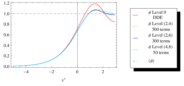
Note that the range is sufficient to compare the different approximations and the different levels (0,0), (2,4), (2,6), (4,8) around the transition to the non-perturbative vacuum, see Fig. 3 as an example for the tachyon only.

Similarly to the level zero solution, Fig. 2, the tachyon is initially in the perturbative vacuum , then grows exponentially near , slightly overshoots the vacuum expectation value , then settles in the non-perturbative vacuum. However using the exponential series ansatz we cannot evaluate the convergence properties around the non-perturbative vacuum. We devote Section 3 to this issue.
All three methods agree very well up to the maximum value near , where the non-linear couplings due to the interaction between the various fields become important. But even for , the solutions are qualitatively very similar.
Let us now consider the solution for the full system of the seven fields at level two that we calculated up to using the exponential series ansatz (16), see Figure 4.

The general picture involving the three stages
holds for all fields. The tachyon is drawn with a thick red brush to emphasize its importance for the vacuum transition: it is the first component to grow, and thus drives the others out of the perturbative vacuum. This affirms the intuitive notion of the tachyon as the unstable mode of the string field, indicating the instability of the supporting D-brane. In addition to the evolution of the seven fields, we included the vevs in the non-perturbative vacuum. In Figure 5 we zoom on the tachyon in order to show how it oscillates around the vev.

Typically one would expect that all fields, except the scalars, have vanishing vev, preserving translation invariance in the non-perturbative vacuum. But due to the presence of the linear dilaton background , translation invariance is broken in the -direction. Hence e.g. is no upset. If , then can have no vev. How exactly the vevs are reached for large is studied in detail in Section 3.
There is more than one way to determine the vevs. The simplest one is the following: Simplify the equations of motion (appendix C) to allow only constant solutions. This results in a set of equations where the vevs appear quadratically, all others linearly, hence there exist solutions. With mathematica they are found in closed form, as expressions depending on roots of 10th order polynomials. Numerically the vevs can be evaluated to arbitrary precision. To pick the right solution from the set of ten, it is sufficient to consider the tachyon vev:
- •
Two solutions can be eliminated as .
- •
Six more can be neglected because . From the effective potential, Fig. 1, we know it is unbounded for negative field values, hence there can be no finite negative vev.
- •
One solution has . The vevs of the other fields vanish, too. This is the unstable, perturbative vacuum solution.
- •
The last is the non-perturbative vacuum solution: . The resulting vevs to four significant digits are summarized in Table 2.
| 0.5416 | 0.8808 | -0.1733 | -0.03670 | 0 | -0.05190 | 0 |
Another way to determine the vevs is to realize that if we expand the string field in the universal basis (i.e. using ghost modes and matter Virasoro modes, but no matter oscillators), the vevs would be independent of the dilaton gradient, and therefore equal to their values in flat spacetime. Using the expression of the Virasoro operators in terms of oscillators and dilaton gradient (61) we can then deduce the vevs of the fields in the non-universal basis. Explicitly, at level two in the universal basis and in Siegel gauge, we have three fields , and , and the string field in the non-perturbative vacuum is given by
| (17) |
where the vevs , and are well known [46]. Plugging the expression (61) for , we have
| (18) |
Comparing with our string field expansion Eq. (7), and the definition of F (9), we find
| (19) |
And these give precisely the same values as in Table 2, providing further evidence that our action was correctly calculated.
A curious result worth mentioning is that the following relations
| (20) |
which, by Eq. (19), should hold for the expectation values, actually hold for all at level (2,4). This can be roughly seen on Fig. 4. We have checked these relations numerically beyond doubt (they hold with a precision of at least 100 digits), but haven’t found any simple reason to explain them. They must in fact be “accidental” because they do not hold anymore at level (2,6).
Let us now briefly look at level (2,6). The main difference here is that we cannot set to zero anymore. In particular, the equation of motion for , which at level (2,4) contained only terms proportional to , now contains in particular a term . We show the exponential series solution for the rolling in Fig. 6

Level four solutions
Let us now turn to the system of equations at level (4,8). Based on the method of conservation laws we used our mathematica code to compute the equations of motion. There are now 50 fields to consider, the equations of motion contain 21400 terms. We want to investigate to what extent the solution changes compared to level two. Again we used the exponential series ansatz and computed the first 50 coefficients for all 50 fields. This calculation took about 15 h on a fast computer. From those 50 fields we decide to focus on the tachyon, discussion of the other 49 fields would be redundant, for they are all qualitatively similar. Now we compare the tachyon at level two and four, Figure 7.
As before the vevs of all fields are extracted from the constant solutions. For the tachyon, the vev is only slightly bigger at level 4, the numerical value agrees with the estimate in [46]. We notice that the tachyon overshoots more at level four, both on a relative scale and in absolute value. As noted in [30], the full solution (no level truncation) converges monotonically. One might have expected to see the overshooting decrease monotonically with the level as well, since it is a lot more pronounced at level zero than at level two, but that is not the case. For completeness, the relative overshooting of the tachyon is shown in Table 3.
| Level | 0 | (2,4) | (2,6) | (4,8) |
|---|---|---|---|---|
| 18.7% | 7.1% | 6.7% | 8.2% |
3 Oscillations around the non-perturbative vacuum
In this section, we want to consider the equations of motions when the fields are very close to their non-perturbative vacuum expectation values. This analysis can be started in a relatively general formalism, independent of the level. We start by putting the components of the string field into a column vector
| (21) |
The length of this vector will be seven at level (2,4), eight at level (2,6), and fifty at level (4,8), the highest level that we consider in this paper. Next we write
| (22) |
where is the non-perturbative vacuum expectation value of , and is a small perturbation. We now write schematically the equations of motion for at linearized level, i.e. keeping only the terms that are linear in . Note that because is a solution of the full equations of motion, there will be obviously no constant term in the linearized equations. The general structure of these equations is easy to understand. On the left hand side, we will write the contributions from the kinetic term; this involves the fields at light-cone time (not retarded) and at most first derivatives of the fields. On the right-hand side we will write the contributions from the interaction term. These all involve the same retarded light-cone time , and at most derivatives, where is the level. This is so because the number of derivatives is at most equal to the total number of Lorentz indices carried by the interacting fields, and each field of level can carry at most indices. So the general form of the equations of motion is
| (23) |
where all the details are hidden in the by matrices and , . We can now make the ansatz
| (24) |
where is a complex number and is a vector of complex numbers. Since the equations (23) are real and linear, we can always find a real solution by adding its complex conjugate to (24). Note that with this ansatz, all fields oscillate with the same frequency with exponentially decaying or growing amplitudes, according to the sign of . The relative amplitudes and phase shifts between the fields are encoded in . Plugging this ansatz into Eq. (23) and multiplying by , we obtain the equation
| (25) |
where is the by identity matrix. After naming
| (26) |
we see that Eq. (25) has a nontrivial solution for if and only if is such that
| (27) |
It is easy to see from (26), that is an exponential polynomial in , i.e. a function of the form
| (28) |
where are polynomials of degree . In our particular case, we have .
So we are interested in finding the roots of an exponential polynomial (27), and particularly in the signs of their real parts because they will determine whether the perturbation will eventually die out or not. This problem has been studied quite extensively (see for example [43]). The general answer is that one can write expressions for the asymptotic values of the zeros (i.e. the zeros with ). More simply, one can use the distribution diagram to approximately locate the zeros. Namely, we plot the points with coordinates ; we then draw the convex polygonal line that joins to , such that its vertices are points of the set and such that no point lies above it. This is illustrated in Fig. 8 for the case of level (2,4).
Now let us denote the successive segments of (from left to right) by , and let denote their slopes. Now the general result [43] is that there exist positive numbers and such that all the zeros with norm greater than , are located inside the union of the strips defined by
| (29) |
It is clear that, for large , these strips are located in the left half-plane if is positive and in the right-half plane if is negative. If , the strip is vertical and contains the imaginary axis. At level (2,4), we have three strips with respectively equal to , , and . These strips are sketched in Fig. 9 .
One can say a little more. In particular, in any region defined by
| (30) |
with no zero on the boundary, the number of zeros in satisfies
| (31) |
where is the number of points of the distribution diagram on and is the difference in values of between the end-points of . In Eq. (30), is an arbitrary real number, and is an arbitrary real positive number. So, for example with (neutral strip), Eq. (30) defines a rectangular box of width and height centered on . Therefore, Eq. (31) just means that the average vertical density of the zeros along the neutral strip is given by . For the other branches with , the picture is almost the same, just a little twisted. But in the limit , is going to be roughly constant in the box, so (30) defines an almost rectangular box centered on . This means in particular that each strip contains infinitely many zeros with arbitrarily large norm. And it has the following immediate consequence: At level (2,4), has infinitely many zeros with arbitrarily large positive real part. This means that if we specify a generic initial condition for the string field , , with close to the non-perturbative vacuum, then we should expect that it will start to oscillate with exponentially growing amplitude, at least until the linear approximation becomes invalid. For concreteness we show, in Figure 9 , the zeros of found numerically in the range . The picture agrees with the asymptotic analysis. We see in particular that the zeros are aligned along branches in each of the strips, and that along these branches the spacing between roots is asymptotically constant. Interestingly, in the retarded strip there is a branch of double roots (the double zeros are plotted in red in Figure 9 ). It turns out that this is related to the fact, already mentioned in Section 2, that at level (2,4) there are only five independent fields because of the relations (20).
In Fig. 8 we have denoted the segment with positive slope as retarded, the one with zero slope as neutral and the one with negative slope as advanced. This denomination is easily understood by looking at the following three simple linear delay differential equations (we refer the reader to Appendix A for definitions and more details on delay differential equations). First, suppose we have an equation of the form
| (32) |
This is an equation of the retarded type since the right-hand-side includes at the retarded time . Making the ansatz , we obtain the characteristic equation for
| (33) |
whose distribution diagram is shown in Fig. 10. It has one segment of positive unit slope; this justifies the denomination “retarded” for such segments.
Now we consider the neutral delay differential equation
| (34) |
which has for characteristic equation . Its distribution diagram, shown in Fig. 10, has one segment of zero slope, hence the denomination “neutral” for such segments. At last, the equation
| (35) |
is of the advanced type because the right-hand side involves at the advanced time . Its characteristic equation is , whose branch diagram is shown on Fig. 10. It has one segment of negative slope, which we therefore name .
To summarize, at level zero the linearized equations of motion are purely of the retarded type because the characteristic equation for the tachyon is [30]:
| (36) |
and its distribution diagram is thus as shown in Fig. 10. From the above discussion, we therefore know that its roots of large absolute value all have negative real part, and it could thus have at most finitely many roots with positive real part. It turns out that all the roots have negative real parts, and the motion around the non-perturbative vacuum is stable at this level. However, we have shown that at level (2,4) we obtain two new segments, a neutral one and an advanced one which ruins the stability around the non-perturbative vacuum. It is interesting to ask what happens at higher levels. We show, in Fig. 11, the distribution diagram found at level (2,6).
Note that at this level, it is not anymore consistent to set to zero, so we have a total of eight fields. One of the most striking differences with level (2,4) is that there is one more advanced segment. This can be understood from the fact that the action at level (2,6) contains higher derivatives at retarded times. One notices also that the retarded segment has become much shorter. With our code, we were able to calculate the action and equations of motion up to level (4,8). From this large calculation we show in Fig. 12 the result for the distribution diagram.
At this level we have fifty fields. It turns out that the calculation of is a difficult problem. With the definition , we see that the entries of the matrix are polynomials in the two variables and . We explain, in Appendix D, why the computation of the determinant of a polynomial matrix is hard and how to overcome this difficulty.
Interestingly, we see that at level (4,8), we have one retarded branch, one neutral branch, and three advanced branches. In this sense, the equations of motion become more and more advanced as the level is increased. We can actually express this idea differently; one could ask if we can write an effective equation of motion for one field, e.g. the tachyon , that would give rise to the same characteristic equation as Eq. (27). The answer is very easy; indeed if we make the ansatz , it is immediately clear that the equation of motion
| (37) |
is precisely the same as Eq. (27), where the ’s are the polynomials defined by Eq. (28). We now do the usual splitting of this differential equation by putting one of the terms with highest derivatives on the left-hand side and all the other ones on the right-hand side. So we choose a such that the degree of the polynomial is maximum (i.e. , ). If the distribution diagram has a neutral segment, then we can choose, for , any along this segment. After subtracting from , the equation of motion thus takes the form
| (38) |
What we can immediately read from this equation is that, at level higher than zero, the non-locality is not anymore concentrated at one point in the past , but instead takes all the values , . While this precise range depends on the value of that we chose, it is clear that it will extend in the future by, at least, an amount equal to the length of the projection of the advanced segments on the axis. And similarly, it will extend in the past by, at least, an amount equal to the length of the projection of the retarded segments on the axis.
If we specify generic initial data for DDEs (38) whose lowest derivative appears at an advanced time (which we call advanced DDEs), we should not expect that smoothing will occur when solving with the method of steps. In fact, we show in Appendix A an example of an advanced DDE which does not even possess a continuous solution for a given initial data. For a system of advanced DDEs, on the other hand, smoothing may occur. For our rolling solution, we require an analytic solution. This is not in conflict with the preceding remark because we are not free to choose any initial data, as we have shown that the initial conditions are essentially uniquely determined by demanding that the tachyon lives in the perturbative vacuum in the infinite light-cone past.
It is clear from the distribution diagrams in Figs. 8 and 12, that and both increase from level (2,4) to level (4,8). Going from level (2,4) to level (2,6), on the other hand, we see that although increases, decreases. But if we look only at levels , we nevertheless still expect that both and will continue to grow beyond level (4,8), and that in the limit , the non-locality extends over the whole discrete range .
At last, we remark that at infinite level, if we subsequently take the limit , which is equivalent to shrinking the delay , the range of non-locality becomes continuous and extends over all light-cone times. We thus recover, in this limit, the non-locality characteristic of usual (zero dilaton) string field theory.
4 Discussion and Conclusions
We have identified the equations of motion for the open string tachyon rolling in a linear dilaton background as being delay differential equations. This class of equations has been widely studied in the mathematics literature. Although no method to analytically solve non-trivial DDEs is known, the method of steps is in general an efficient numerical method (and essentially the only method) once the initial data is provided. We have used this method in order to solve the equations of motion at level zero, and found that it is both efficient and accurate; in particular our solution agrees very well with the results from an exponential series ansatz, and can be continued much further in light-cone time (Fig. 2).
At truncation level two, we found that the method of steps can be used only when we further truncate the action by either removing all higher derivatives, or by keeping only the scalar fields. But we saw that the results from these approximations all agree reasonably well with the more accurate solution from the exponential series ansatz, at least until the first maximum has been reached (Fig. 3). The obtained numerical solutions can be continued for much larger light-cone time, where it is seen that they converge towards the non-perturbative vacuum. If we don’t simplify the equations of motion, our numerical solver gives us wrong solutions. We have understood that this problem is due to the fact that our equations of motion possess derivatives of order higher than one at retarded times. In general, such equations are not even guaranteed to possess continuous solutions. While we still expect the equations of motion to have an analytic solution for the initial data corresponding to a tachyon in the perturbative vacuum in the far light-cone past, the method of steps is rendered unstable by the higher derivatives.
We have already mentioned that the diffusion equation method [36, 37, 38] has been successfully used to solve numerically the light-like rolling problem at level zero [35]. It is then natural to ask wether this method can give more stable solutions at higher levels. The diffusion method has the virtue of applying to a larger class of non-local equations. But in the case of DDEs, we believe that it is completely identical to the method of steps. It would then face exactly the same problem as the method of steps at higher levels. To illustrate this, we briefly review the diffusion method applied to the equation
| (39) |
First we define a function of two variables and by This definition is implemented by the simple diffusion equation
| (40) |
The idea is then to solve the diffusion equation on the region and . The subtle part is to determine the boundary conditions. It turns out that the boundary conditions on the axis are determined by the equation (which is now local in ):
| (41) |
A simple algorithmic resolution of the diffusion equation is the following:
- 1.
Specify boundary conditions on the segment . This is the initial data.
- 2.
- 3.
To solve the diffusion equation further, one needs first to specify the initial conditions on the segment defined by and using Eq. (41). Since the simple diffusion equation has been solved exactly in the previous step, replace by , and the right-hand side is simply the initial data. One obtains precisely the original equation (39) (with replaced by ).
- 4.
Solve again the diffusion equation by copying the obtained boundary values on the segment and to the segment and .
- 5.
Solve again Eq. (41) on the segment and . From the same argument as above, plus the fact that one can replace the right-hand side of (41) by , this is solving the DDE equation (39) on the interval given the values of on the interval . This is precisely the method of steps as described in Appendix A!
The algorithm then continues by repeating points 4 and 5, which is equivalent to solving the original DDE (39) by the method of steps.
To summarize, the diffusion method applied to a DDE “mimics” the method of steps. We cautiously note, however, that a different numerical method to solve the diffusion equation may change the above claim if Eq. (40) is not solved exactly as in our algorithm.
In order to find accurate numerical solutions taking all derivatives into account, we had to resort to the exponential series ansatz. This method generalizes obviously from level zero; in particular one still can calculate recursively the coefficients of the series. The problem with this method is that the number of coefficients needed grows exponentially with the light-cone time until which we want our solution to be accurate. Moreover, we must calculate the coefficients with many digits precision in order to account for the numerical cancellation errors. At levels (2,4) (Figs. 4 and 5) and (2,6) (Fig. 6) we were nevertheless able to find solutions that are accurate up to a point where the string field is convincingly seen to converge towards the non-perturbative vacuum. Moreover, we have found that the convergence (as measured by the overshooting of the first maximum) is substantially faster at levels two and four than at level zero. At level four, it is a little bit slower that at level two (Fig. 7). In order to compare this to the analytic solution of Hellerman and Schnabl [30], it is instructive to look at the tachyon component of their solution (in Schnabl gauge). Normalizing the tachyon vev in the non-perturbative vacuum to one, it is
| (42) |
a monotonic solution. So the fact that our solution at level two has become more monotonic is a good indication that level truncation yields qualitatively the same solution (in Siegel gauge). We note, however, that if we expand (42) as a power series in (what we have called an exponential series), it has a finite radius of convergence; the series diverges for . On the other hand, the exponential series that we obtained have a much larger radius of convergence, perhaps infinite as can be shown at level zero from the asymptotic behavior of the coefficients of the series [30]. It is worth mentioning a curious fact. Had we taken the level-zero equation of motion (with vev normalized to unity) , and dropped the delay , we would get
which has the solution
Precisely the same as (42)! This might just be a coincidence; it could also point at something deeper which may be worth examining in a further work.
To sum up, our numerical solutions at levels two and four strongly indicate that the string field will eventually converge to the non-perturbative vacuum, in agreement with the analytic solution of [30]. On the other hand, we have also shown that, at levels higher than zero, the equations of motion, linearized around the non-perturbative vacuum, admit infinitely many oscillating solutions with exponentially growing amplitude. This suggests that the string field should not converge to this vacuum. These two apparently contradictory results can be reconciled in different ways. Below we describe two possibilities.
The first possibility is that the string field somehow avoids the infinitely many exponentially growing modes. This is certainly possible because the initial conditions (i.e. the string field sitting in the perturbative vacuum in the infinite light-cone past) are very special: With this point of view, we should conclude that the motion is unstable: should an external perturbation, or a quantum effect, move the string field the tiniest bit away from this particular solution it would not converge. We should also stress that our analysis of the linearized equations of motion doesn’t tell us how non-convergent the rolling would be. It might approach a limit cycle (in phase space) as is sometimes the case when the linearized equations of motion have a finite number of growing solutions. Our situation, however, is different because we have infinitely many growing solutions in the vacuum. This could render the rolling diverging. Or it might not be that bad; after all, we could imagine expressing a well-behaved converging function as a series in the infinitely many diverging modes [43]; this would not be possible in the finite case. We emphasize here again the special character of the initial condition of the tachyon sitting on the top of the hill in the infinite light-cone past, which we have shown uniquely fixes the initial data up to a shift in light-cone time. The method of exponential series, which gives a convergent solution, can work only with this particular initial condition, which is also the initial condition of the analytic solution of [30]. For a generic initial condition the coefficients cannot be determined recursively, because “negative” modes have to be taken into account. In the level zero case, with , one obtains
| (43) |
In other words: in order to calculate one coefficient, we need to know all coefficients, including the one we are interested in! The same problem is found in the DDE approach: to find initial data that are consistent with the equation of motion, we need to solve the very same equation of motion. This is a simple problem only when we require that the tachyon be in the non-perturbative vacuum in the infinite past.
We leave it for further work to study different initial conditions. At level zero it was done in [35]; but at higher levels we expect different results due to the higher derivatives and divergent modes.
A second possibility to reconcile a convergent rolling solution with infinitely many growing modes is that these modes do not satisfy the ‘‘out-of-gauge’’ equations of motion66 6 We thank T. Erler and M. Schnabl for emphasizing this point to us.. Indeed we have derived the equations of motion from the gauge-fixed action. This means that for a solution , we are guaranteed that for all in Siegel gauge. But it is possible that itself doesn’t vanish. That such solutions can exist was shown in [47].
The two different explanations above differ in particular by the interpretation of the growing modes. In the first possibility, they do have some physical meaning and make the rolling unstable. While we do not expect to find open string degrees of freedom in the non-perturbative vacuum, it is not unreasonable to think that the unstable modes could correspond to the closed tachyon instability. After all, we have coupled the open string field theory to the closed sector, although only via the dilaton. In the second possibility mentioned above, however, the growing modes are simply unphysical because they do not obey the out-of-gauge equations of motion. In order to find out if this is the case, we would have to derive the equations of motion from the gauge-unfixed action and verify whether the growing modes are still solutions of these full equations of motion. We hope to be able to report on this in a future publication. The present paper gives only a partial answer to the question of the physical meaning of the growing modes. At the end of Section 3, we wrote an effective equation of motion for one scalar field, whose solutions are precisely the exponential modes solutions of the whole system of equations of motion linearized around the non-perturbative vacuum. We have then found that the decaying modes correspond to positive delays in the effective equation of motion, thus non-locality in the past, and that growing modes correspond to negative delays, i.e. non-locality extending into the future.
Acknowledgments.
We extend our sincere gratitude to T. Erler for useful discussions, and to N. Barnaby and M. Schnabl for insightful comments on the manuscript. We are indebted to A. Golovnev for providing us with a copy of Ref. [3]. N. M. is supported in parts by the Transregio TRR 33 ’The Dark Universe’ and the Excellence Cluster ’Origin and Structure of the Universe’ of the DFG.Appendix A Delay differential equations
Differential equations describing real life systems like chemical reactions, predator-prey relations, etc… often need to incorporate the state of the system not only now, but also at times in the past. A simple example is the following delay differential equation (DDE)
| (44) |
with the constant delay term . Notice the non-locality: the derivative is needed at , but the function itself is evaluated a finite distance away at . This equation is of the retarded type. In order to make this a well posed problem it is not sufficient to look for a solution starting at a point with the value of the function fixed as in the Cauchy initial value problem for an ordinary differential equation (ODE). Instead one has to supply the initial data over a continuous range of points. Choosing for example one has as a well posed problem
In contrast to an ODE problem the solution to the above problem has discontinuity points of order n where the -th derivative is discontinuous. One can quickly see how this comes about. Approaching 0 from the left, , however approaching from the right one finds
This discontinuity propagates further along the solution. The second derivative at reads
and is thus discontinuous. However, the first derivative at is , which is continuous. Hence the solution is of class at This process continues at every positive integer , where the solution is ; hence the discontinuities are smoothed out as increases. The propagation and existence of discontinuity points is a generic feature of DDEs. In general the solution only links continuously with the initial data at the starting point .
Consider as a second example a DDE of the advanced type
| (45) |
The only variation to (44) is that the derivative is taken at the present instant, but the function is needed at a future point. For we have and similarly the solution vanishes for all positive . The solutions to both examples, (44) and (45), are plotted in Figure 14. The discontinuity of the advanced solution at is noteworthy: for this type of equation only special initial conditions allow for a continuous solution. In our example that special choice among the class of constant initial data is .
The above examples can be generalized further to include any number of delays, possibly variable or time dependent delays or even state dependent delays . If there are derivative terms at delayed points, the equation is said to be of the neutral type (NDDE). In general the delay functions and can be completely independent. If depends on over a continuous range, the problem is called a Volterra functional differential equation, but for the present purpose, one can restrict to only a finite number of points in the past required to compute the current rate of change in the system.
The general definition of a first-order delay differential equation problem then reads
Extending to systems of DDEs or higher order derivative terms is then straightforward. There are further major differences between ODEs and DDEs in addition to the above discussed discontinuities.
- •
Different initial data can give rise to the same solution
- •
The solution may be non-unique in the state dependent case
- •
The solution may terminate at a point
- •
In the neutral case generally no smoothing of discontinuities occurs
- •
Bounded solutions may oscillate or show chaotic behavior even in the one-dimensional case, while ODEs can oscillate only in at least two dimensions and behave chaotically in at least three dimensions (Poincaré-Bendixson theorem). In fact oscillations are typical of DDEs
- •
infinitesimal delays introduced into ODEs can stabilize or destabilize the solution
- •
For scalar NDDEs no smoothing occurs, but for systems of NDDEs smoothing may take place
Existence and Uniqueness
Theorems on local existence and uniqueness have been developed for very general assumptions on the delay functions and . But for the case at hand in this paper one can use familiar results from ODE theory. Assume there is only one delay, a positive number on the interval of interest
This case of constant delay then reduces to the following ordinary differential equation initial value problem on the interval between the initial point and the corresponding point shifted by one delay
Standard results then guarantee local existence and uniqueness of a continuous solution in for some provided that is continuous with respect to , Lipschitz continuous with respect to and that are themselves Lipschitz continuous. Note however that there exists a whole family of discontinuous solutions, linked to the unique continuous one by a constant offset.
Method of steps
In order to obtain the solution on the full interval it is convenient both theoretically and computationally to iterate along the intervals , using the solution calculated for the previous interval. This is known as the method of steps, the principal algorithm to solve DDEs numerically. It is applicable in the case where all discontinuity points are known in advance, e.g. for a constant delay. Solving the DDE then reduces to solving ODEs on the intervals between two discontinuity points using standard ODE methods such as linear multistep solvers and gluing the solution together at the interval boundaries. For continuing over several such intervals the ODE method has to supply a continuous (polynomial) interpolation of the solution which matches the accuracy order of the solver. For concreteness, let be the solution on the interval , then for the solution in the next step the ODE reads
Appendix B Lagrangian at level (2,4)
We present the full Lagrangian density with fields up to level two and interaction terms up to level four in the linear dilaton background with light-like dilaton gradient . The Lagrangian can be split into two: one is explicitly -dependent and vanishes for , the other survives for . While could always be eliminated using the modified momentum conservation , we keep it explicit for easier comparison with [41]. The interaction term can be split up according to the level and the number of derivatives , . Overall we have
We use the following expansion of the string field into Fock space states
Working in the light-cone, we have
and for example
We split the Lorentz indices into light-like and ordinary components
In order to simplify the equations of motion, we need not consider all 379 independent components of from the expansion (where is symmetric). Several facts aid in reducing the number of fields:
- 1.
Any symmetric tensor can be reduced to a traceless and a pure trace part: with traceless.
- 2.
For any field , it only appears in the action coupled to another field . Thus we can safely set these fields to zero and trivially satisfy their equations of motion, but still allow for a non-trivial solution for the remaining fields.
We end up with the following eight fields to solve for:
Fields with a tilde are defined by
Explicitly the kinetic and interaction without the extra dilaton contribution contain the following 41 terms: 77 7 For brevity we set .
In addition we obtain eight interaction terms and four kinetic terms from introducing the dilaton. The kinetic terms however do not contribute to the equations of motion, they are essentially total derivatives.
| Writing the action explicitly in terms of these eight fields gives the Lagrangians: | |||
Appendix C Equations of motion at level (2,4)
With the solution and the retarded point , the seven remaining equations of motion become:
Equation of motion for the tachyon (48 terms):
Equation of motion for (30 terms):
Equation of motion for (12 terms):
Equation of motion for (11 terms):
Equation of motion for (11 terms):
Equation of motion for (20 terms):
Equation of motion for (12 terms):
Appendix D Determinant of polynomial matrices
In this paper, we have to evaluate the determinant of a matrix whose entries are polynomials in two variables and . The result is obviously a polynomial in and as well. One could of course use the traditional methods, for example LU decomposition, but one then notices that the complexity of the calculation grows very fast with the matrix size. This is easy to understand when one notes that such methods require the matrix to be over a field. One will then have to think of elements of as rational functions of and . The calculation of the determinant will then involve potentially heavy computations on large fractions. Moreover, since the determinant is a polynomial, the end result will involve a large simplification between numerator and denominator, meaning that we might be doing many more calculations than necessary. In fact we observed that, while mathematica can calculate such a determinant for a seven by seven matrix, it fails to do so for a fifty by fifty matrix whose entries are polynomials of degrees at most eight in and at most one in . This prompted us to look for alternative methods.
An elegant method [48] is based on the discrete Fourier transform. We mention also that there is another method [49], that can efficiently calculate the degree of the determinant. This is in fact what we need, but it is unclear to us how to generalize this method to polynomial matrices in several variables, so we will use the first method based on the Fourier transform.
To explain this method, it will be enough to concentrate on the case of polynomials in one variable ; the generalization to several variables will then be obvious. The crucial fact to realize is that polynomial multiplication is, in some sense, a convolution. More explicitly, let’s consider two polynomials and of degrees and
| (46) |
We define and we write the coefficients and into vectors and , both of length .
| (47) |
where for and for . We can then write the product also in a vector of the same length because it has degree . The components of are then given by . If we define the negative components of and by imposing the periodicity (and similarly for and ), we can extend the summation to the whole range
| (48) |
This in fact doesn’t change the sum because all additional terms are zero; but in the form (48), one recognizes that is the cyclic convolution of and
| (49) |
We can now use the fact that the discrete Fourier transform defined by
| (50) |
changes cyclic convolution into multiplication. Namely
| (51) |
where the multiplication of two vectors is done component-wise. One can then perform an inverse discrete Fourier transform to obtain .
Let us now consider, for a little while, the Leibniz formula for the determinant of the square matrix of size
| (52) |
We estimate an upper bound on the degree of and write its coefficients in the vector of length ; and we also write the coefficients of in vectors , each of length . We can now write the polynomial product in (52) as a usual product of the components of the discrete Fourier transforms of
| (53) |
Now if we define the matrices by
| (54) |
the Leibniz formula becomes
| (55) |
In other words, the components of are the determinants of the matrices whose entries are numbers; these determinants can therefore be calculated with a standard method. To summarize, the algorithm to calculate the determinant of is:
- 1.
Find an upper bound on the degree of .
- 2.
Calculate the matrices for , whose entries are the components of the discrete Fourier transform of the entries of .
- 3.
Calculate the determinants of the matrices . These are the components of .
- 4.
Inverse discrete Fourier transform in order to find the coefficients of the polynomial .
We make a few comments. First, it is well known that the discrete Fourier transform can be made extremely fast with the Fast Fourier Transform algorithm, so this method is relatively efficient. On the other hand, if one is interested in determining the degree of , numerical errors can make it hard to decide whether a term appearing in the answer for the determinant, with a very small number in absolute value, should be kept or whether it comes from numerical imprecision. For this reason, it might be necessary to run the algorithm with a precision of many digits. At last, this algorithm generalizes almost trivially to polynomials in several variables; the discrete Fourier transforms have then to be replaced by multidimensional discrete Fourier transforms.
Appendix E Review of linear dilaton CFT
In the following we want to review briefly how the linear dilaton CFT arises and quote the most useful results that are needed to compute correlators and the equations of motion in a linear dilaton background. A similar, even shorter overview can be found in [30], Section 2. Much more is covered in [50], Sections 2.5, 2.7 and 3.7, where additionally the role of the dilaton field in string interactions is illuminated.
Let’s start by considering the description of string theory in curved spacetime. After all string theory is supposed to give a framework for quantum gravity. As a reminder the Polyakov action that serves as the starting point for string theory is
As a natural extension one is tempted to replace the flat Minkowski metric with a general metric . Considering spacetime as a coherent background of gravitons is slightly dubious, as it means string theory is formulated in a background of strings. But let’s try anyway. If we add the graviton background we might as well add the background from the two other closed string massless states, the antisymmetric tensor and the dilaton , resulting in a so called nonlinear sigma model action
where are the worldsheet metric and curvature.
If we now demand this action to be Weyl invariant also at the quantum level the corresponding -functions for of the renormalization group flow have to vanish (scale invariance). To first order in , only derivatives of the dilaton appear in the -functions. This means changing the dilaton by a constant is allowed. A constant shift in yields a contribution proportional to the worldsheet Euler number , defined as
In fact the Euler number determines the interaction strength, such that the open string coupling constant is related to the expectation value of the dilaton by
Typically in quantum field theory the coupling is a free parameter, so different values for the coupling represent different theories in sharp contrast to string theory: different coupling is just a different background of the same theory. However since we cannot determine these background values from the dynamics, this distinction moves the difficulty elsewhere, but in principle, there is no free parameter as in QFT.
If the dilaton is not constant, then in order to preserve Weyl invariance, the critical dimension of the string theory may be altered. One choice of fields that preserves Weyl invariance is
where is linear in (linear dilaton), and the constant vector is the dilaton gradient. It singles out a particular direction in spacetime, breaking spacetime translation symmetry. Momentum conservation is then modified as
| (56) |
The functions vanish if
Conversely the central charge of this theory is
Hence different values of the dilaton gradient give different CFTs. We will choose a light-like dilaton gradient, , then the central charge and critical dimension are unaffected.
The complete (Euclidean) action for the linear dilaton on worldsheet with boundary then becomes
| (57) |
where denotes the worldsheet boundary curvature. Varying the action with respect to the metric gives the energy-momentum tensor
| (58) |
the usual expression with an additional dependent contribution.
Gauge fixing the metric permits obtaining the same metric as before on the complex plane, such that the gauge fixed action has the same form as in the free theory with :
| (59) |
This theory deserves the name CFT, for the action (59) is invariant under the conformal change of coordinate , where the field transforms as
| (60) |
Note that this transformation has again an extra piece containing the dilaton gradient. We want the (real) boundary of the upper half plane to be mapped into itself so we can use the doubling trick and , thus we require . Denoting the real coordinate with in contrast to complex , a boundary field transforms as
with the visible difference that the s have disappeared. Expanding the energy-momentum tensor into Laurent modes, we find the new (matter) Virasoros
| (61) |
The conformal weights of any operator can be determined from the OPE with the energy-momentum tensor. For example, the weight of is
On the boundary, things are a little more complicated. The normal ordering
is just valid in the bulk, not on the boundary. On the real line the Green’s function needs to be modified (call it ) to satisfy the Neumann boundary conditions . This is accomplished by an additional image charge term
| (62) |
Normal ordering should remove the divergence of this Green’s function at zero separation, but the usual subtraction is not enough, it only cancels the first divergent term, thus it has to be doubled. The new prescription goes by the name of boundary normal ordering, distinguished from the bulk conformal normal ordering by new symbols ,
We stress again that the reason for introducing another normal ordering is just to have well-behaved (finite) expectation values for products of boundary normal ordered operators.
When taking real derivatives of boundary operators, factors of 2 need to be taken into account because . This is a source of great confusion. Furthermore operators on the boundary may also have different weights from their “relatives” defined on the interior/bulk because of that, e.g. has weight
| (63) |
It is instructive to check the consistency: the linear dilaton is a background field, thus non-dynamical. If we set in the above formulae the free string theory is recovered, as it should.
References
- [1] A. Neveu, H. Nicolai and P. C. West, “New Symmetries And Ghost Structure Of Covariant String Theories,” Phys. Lett. B 167, 307 (1986).
- [2] E. Witten, “Noncommutative Geometry And String Field Theory,” Nucl. Phys. B 268, 253 (1986).
- [3] M. Ostrogradski, “Mémoires sur les équations différentielles relatives au problème des isopérimètres,” Mem. Ac. St. Petersbourg VI 4, 385 (1850).
- [4] D. A. Eliezer and R. P. Woodard, “The Problem of Nonlocality in String Theory,” Nucl. Phys. B 325, 389 (1989).
- [5] C. M. Bender and P. D. Mannheim, “No-ghost theorem for the fourth-order derivative Pais-Uhlenbeck oscillator model,” Phys. Rev. Lett. 100, 110402 (2008) [arXiv:0706.0207 [hep-th]].
- [6] J. A. Minahan, “Quantum corrections in p-adic string theory,” arXiv:hep-th/0105312.
- [7] L. Brekke, P. G. O. Freund, M. Olson and E. Witten, “Nonarchimedean String Dynamics,” Nucl. Phys. B 302, 365 (1988).
- [8] N. Barnaby and N. Kamran, “Dynamics with Infinitely Many Derivatives: The Initial Value Problem,” JHEP 0802, 008 (2008) [arXiv:0709.3968 [hep-th]].
- [9] G. Calcagni, M. Montobbio and G. Nardelli, “Localization of nonlocal theories,” Phys. Lett. B 662, 285 (2008) [arXiv:0712.2237 [hep-th]].
- [10] A. Sen, “Rolling Tachyon,” JHEP 0204, 048 (2002) [arXiv:hep-th/0203211].
- [11] A. Sen, “Tachyon matter,” JHEP 0207, 065 (2002) [arXiv:hep-th/0203265].
- [12] N. Moeller and B. Zwiebach, “Dynamics with infinitely many time derivatives and rolling tachyons,” JHEP 0210, 034 (2002) [arXiv:hep-th/0207107].
- [13] M. Fujita and H. Hata, “Time dependent solution in cubic string field theory,” JHEP 0305, 043 (2003) [arXiv:hep-th/0304163].
- [14] H. t. Yang, “Stress tensors in p-adic string theory and truncated OSFT,” JHEP 0211, 007 (2002) [arXiv:hep-th/0209197].
- [15] L. Joukovskaya, “Dynamics with Infinitely Many Time Derivatives in Friedmann-Robertson-Walker Background and Rolling Tachyon,” JHEP 0902, 045 (2009) [arXiv:0807.2065 [hep-th]].
- [16] E. Coletti, I. Sigalov and W. Taylor, “Taming the tachyon in cubic string field theory,” JHEP 0508, 104 (2005) [arXiv:hep-th/0505031].
- [17] M. Kiermaier, Y. Okawa and B. Zwiebach, “The boundary state from open string fields,” arXiv:0810.1737 [hep-th].
- [18] B. Zwiebach, “Oriented open-closed string theory revisited,” Annals Phys. 267, 193 (1998) [arXiv:hep-th/9705241].
- [19] B. Zwiebach, “Closed string field theory: Quantum action and the B-V master equation,” Nucl. Phys. B 390, 33 (1993) [arXiv:hep-th/9206084].
- [20] A. Belopolsky, “Effective Tachyonic potential in closed string field theory,” Nucl. Phys. B 448, 245 (1995) [arXiv:hep-th/9412106].
- [21] N. Moeller, “Closed bosonic string field theory at quartic order,” JHEP 0411, 018 (2004) [arXiv:hep-th/0408067].
- [22] H. Yang and B. Zwiebach, “Dilaton deformations in closed string field theory,” JHEP 0505, 032 (2005) [arXiv:hep-th/0502161].
- [23] H. t. Yang and B. Zwiebach, “Testing closed string field theory with marginal fields,” JHEP 0506, 038 (2005) [arXiv:hep-th/0501142].
- [24] H. Yang and B. Zwiebach, “A closed string tachyon vacuum?,” JHEP 0509, 054 (2005) [arXiv:hep-th/0506077].
- [25] N. Moeller and H. Yang, “The nonperturbative closed string tachyon vacuum to high level,” JHEP 0704, 009 (2007) [arXiv:hep-th/0609208].
- [26] N. Moeller, “Closed bosonic string field theory at quintic order: Five-tachyon contact term and dilaton theorem,” JHEP 0703, 043 (2007) [arXiv:hep-th/0609209].
- [27] N. Moeller, “Closed bosonic string field theory at quintic order. II: Marginal deformations and effective potential,” JHEP 0709, 118 (2007) [arXiv:0705.2102 [hep-th]].
- [28] N. Moeller, “A tachyon lump in closed string field theory,” JHEP 0809, 056 (2008) [arXiv:0804.0697 [hep-th]].
- [29] B. Zwiebach, “Quantum open string theory with manifest closed string factorization,” Phys. Lett. B 256, 22 (1991).
- [30] S. Hellerman and M. Schnabl, “Light-like tachyon condensation in Open String Field Theory,” arXiv:0803.1184 [hep-th].
- [31] S. R. Coleman, “The Fate Of The False Vacuum. 1. Semiclassical Theory,” Phys. Rev. D 15, 2929 (1977) [Erratum-ibid. D 16, 1248 (1977)].
- [32] M. Schnabl, “Comments on marginal deformations in open string field theory,” Phys. Lett. B 654, 194 (2007) [arXiv:hep-th/0701248].
- [33] M. Kiermaier, Y. Okawa, L. Rastelli and B. Zwiebach, “Analytic solutions for marginal deformations in open string field theory,” JHEP 0801, 028 (2008) [arXiv:hep-th/0701249].
- [34] M. Schnabl, “Analytic solution for tachyon condensation in open string field theory,” Adv. Theor. Math. Phys. 10, 433 (2006) [arXiv:hep-th/0511286].
- [35] N. Barnaby, D. J. Mulryne, N. J. Nunes and P. Robinson, “Dynamics and Stability of Light-Like Tachyon Condensation,” JHEP 0903, 018 (2009) [arXiv:0811.0608 [hep-th]].
- [36] G. Calcagni and G. Nardelli, “Tachyon solutions in boundary and cubic string field theory,” Phys. Rev. D 78, 126010 (2008) [arXiv:0708.0366 [hep-th]].
- [37] G. Calcagni and G. Nardelli, “Kinks of open superstring field theory,” Nucl. Phys. B 823, 234 (2009) [arXiv:0904.3744 [hep-th]].
- [38] G. Calcagni and G. Nardelli, “String theory as a diffusing system,” arXiv:0910.2160 [hep-th].
- [39] P. M. Ho and S. Y. Shih, “Discrete States in Light-Like Linear Dilaton Background,” JHEP 0801, 054 (2008) [arXiv:0711.2792 [hep-th]].
- [40] L. Rastelli and B. Zwiebach, “Tachyon potentials, star products and universality,” JHEP 0109, 038 (2001) [arXiv:hep-th/0006240].
- [41] V. A. Kostelecky and S. Samuel, “On a Nonperturbative Vacuum for the Open Bosonic String,” Nucl. Phys. B 336, 263 (1990).
- [42] T. Erler, “Level truncation and rolling the tachyon in the lightcone basis for open string field theory,” arXiv:hep-th/0409179.
- [43] R. Bellman and K. L. Cooke, “Differential-Difference Equations,” Mathematics in Science and Engineering, Vol. 6, Academic Press Inc. (London) Ltd. 1963.
- [44] R. D. Driver, “Ordinary and Delay Differential Equations,” Applied Mathematical Sciences 20, Springer Verlag, 1977.
- [45] A. Bellen and M. Zennaro, “Numerical Methods for Delay Differential Equations,”Numerical mathematics and scientific computation, Oxford Science Publications, 2003.
- [46] A. Sen and B. Zwiebach, “Tachyon condensation in string field theory,” JHEP 0003, 002 (2000) [arXiv:hep-th/9912249].
- [47] H. Hata and S. Shinohara, “BRST invariance of the non-perturbative vacuum in bosonic open string field theory,” JHEP 0009, 035 (2000) [arXiv:hep-th/0009105].
- [48] P. Kujan, M. Hromčík, M. Šebek, N. Karampetakis, E. Antoniou and S. Vologiannidis, “Effective computations with 2-variable polynomial matrices in Mathematica,” 12th IEEE Mediterranean Conference on Control and Automation, June 6-9, 2004, Kusadasi, Aydin, Turkey.
- [49] D. Henrion and M. Šebek, “Improved Polynomial Matrix Determinant Computation,” IEEE Trans. on CAS - Pt I. Fundamental Theory and Applications, Vol. 46, No. 10, pp. 1307-1308, October 1999.
- [50] J. Polchinski, “String theory. Vol. 1: An introduction to the bosonic string,” Cambridge, UK: Univ. Pr. (1998) 402 p.