跳到论文正文
W Papers独立论文阅读器 arXiv:0912.1076 论文正文 计算阅读时间 · 0%
引用这篇论文根据当前论文元数据生成,正式投稿前建议核对。


License: arXiv.org perpetual non-exclusive license
arXiv:0912.1076v1 [hep-ph] 06 Dec 2009

Contributions to the Muon’s Anomalous Magnetic Moment from a Hidden Sector

Preprint: EFI 09-33
David McKeen Email: mckeen@theory.uchicago.edu Affiliation: Enrico Fermi Institute and Department of Physics, University of Chicago, 5640 South Ellis Avenue, Chicago, IL 60637
August 24, 2026
Abstract

The measurement of the anomalous magnetic moment of the muon provides a stringent test of the standard model and of any physics that lies beyond it. There is currently a deviation of 3.1​σ3.1\sigma between the standard model prediction for the muon’s anomalous magnetic moment and its experimental value. We calculate the contribution to the anomalous magnetic moment in theories where the muon couples to a particle in a hidden sector (that is, uncharged under the standard model) and a connector (which has nontrivial standard model gauge and hidden sector quantum numbers).

pacs
12.60.–i, 13.40.Em, 14.60.Hi, 14.80.–j

I Introduction

Quantum field theory predicts that the gyromagnetic ratio of the muon will differ slightly from its tree-level value of gμ=2g_{\mu}=2. Properly accounting for the nonzero value of the anomalous magnetic moment, aμ=(gμ−2)/2a_{\mu}=(g_{\mu}-2)/2, of the muon is a precise test of the standard model (SM) and of physics beyond the SM.

The most recent determination of aμa_{\mu} in the SM is [1]

aμSM=(11​659​183.4±4.9)×10−10.\displaystyle a_{\mu}^{\rm SM}=\left(11~659~183.4\pm 4.9\right)\times 10^{-10}~~~. (1)

The dominant sources of uncertainty in this expression are the leading-order hadronic vacuum polarization contribution and the contribution from hadronic light-by-light scattering. In Ref. [1], the leading-order hadronic contribution is determined to be

aμLO​Had.=(695.5±4.1)×10−10,\displaystyle a_{\mu}^{\rm LO~Had.}=\left(695.5\pm 4.1\right)\times 10^{-10}~~~, (2)

while the most recent determination of the hadronic light-by-light contribution is [2]

aμHad.LbL=(10.5±2.6)×10−10.\displaystyle a_{\mu}^{\rm Had.~LbL}=\left(10.5\pm 2.6\right)\times 10^{-10}~~~. (3)

The total SM prediction for aμa_{\mu} in Eq. 1 differs from the experimental value [3],

aμExp=(11​659​208.0±5.4±3.3)×10−10,\displaystyle a_{\mu}^{\rm Exp}=\left(11~659~208.0\pm 5.4\pm 3.3\right)\times 10^{-10}~~~, (4)

at the 3.1​σ3.1\sigma level. There is some discrepancy in using e+​e−e^{+}e^{-} or τ\tau decay data to extract the leading-order hadronic contribution to aμa_{\mu} with τ\tau decay data leading to a 1.9​σ1.9\sigma difference between the SM and experimental values of aμa_{\mu}. For recent reviews of the status of aμa_{\mu}, see Ref. [4]

The difference between aμSMa_{\mu}^{\rm SM} and aμExpa_{\mu}^{\rm Exp} has spurred numerous studies of new physics scenarios that could offer an explanation, for example, supersymmetry [5], universal extra dimensions [6], and unparticles [7]. Another scenario that has received attention in the literature is that of a hidden U​(1)′U(1)^{\prime} whose gauge boson kinetically mixes with the photon [8]. The constraints from aμa_{\mu} on such a scenario are discussed in [9].

In this paper we investigate and catalogue the contributions to aμa_{\mu} that arise from the muon coupling to some hidden sector. We do this in four situations that differ in the spin of the hidden sector particle that couples to the muon, and in the spin of other particles present in the interaction to preserve gauge invariance. These scenarios are generalizations of some models already investigated, like that of [9].

Schematically, the interactions we consider are of the form

ℒint∼λ​X​Y​μ,\displaystyle{\cal L}_{\rm int}\sim\lambda XY\mu~~~, (5)

where Lorentz and gauge indices have been suppressed. In this Lagrangian and in the rest of this work, XX refers to a SM singlet that could be charged under some hidden symmetry group, which we denote by GG, and YY is a particle that is charged under the SM (to preserve the SM gauge invariance of the interaction) and under GG if XX is (to preserve GG invariance). The particles in Eq. 5 are classified in the table below:

Type of matter Std. Model G Example
Ordinary Non-singlet Singlet μ\mu
Connector Non-singlet Non-singlet YY
Hidden Singlet Non-singlet XX

λ\lambda is the coupling strength of this interaction between the muon, the hidden sector particle XX, and the connector YY. Interactions of this form generate corrections to aμa_{\mu} of order λ2\lambda^{2}.

We note that XX could be a dark matter candidate. If mX<mYm_{X}<m_{Y} and XX is the lightest particle with some hidden charge, it could be long lived. Indeed, the relic density of XX could naturally be driven to the observed value of ΩX≃0.23\Omega_{X}\simeq 0.23 although its mass is unconnected to the electroweak scale in a WIMPless dark matter scenario [10]. For XX to be a viable dark matter candidate, it cannot be coupled too strongly to the SM; that is λ ∼<gweak\lambda\mathrel{\hbox to0.0pt{\lower 4.0pt\hbox{\hskip 1.0pt$\sim$}\hss}\raise 1.0pt\hbox{$<$}}g_{\rm weak}. Of course, this condition is relaxed if we do not require that XX comprise the most of the dark matter density. These scenarios have been studied in situations where XX couples to bb quarks, leading to an explanation of the DAMA/LIBRA signal [11] and to missing energy in decays of mesons with bb quarks [12].

In Sec. II, we discuss constraints on XX and YY from collider experiments. In Sec. III, we present the contributions to aμa_{\mu} due to several scenarios of the form of Eq. 5. We discuss constraints from the measured value of aμa_{\mu} on these scenarios in Sec. IV, and, in Sec. V, we conclude.

II Collider constraints on XX and YY

If XX is a SM singlet that is only weakly coupled to the SM, as we assume here, then there are no firm constraints on its allowed mass coming from collider experiments. We consider its mass to be essentially free in this study.

There are, however, tight bounds on the possible mass of YY since it has the same electric charge as the muon. The firmest bounds come from the LEP experiments’ searches for right-handed sleptons. These experiments looked for a pair of sleptons produced by a virtual photon or ZZ that decay to a pair of acoplanar leptons along with two neutralinos (missing energy). Such searches apply in the case of a Lagrangian of the form of Eq. 5 if mX<mY−mμm_{X}<m_{Y}-m_{\mu} and λ\lambda large enough that the YY’s decay promptly, that is, λ ∼>10−8\lambda\mathrel{\hbox to0.0pt{\lower 4.0pt\hbox{\hskip 1.0pt$\sim$}\hss}\raise 1.0pt\hbox{$>$}}10^{-8}.

The ALEPH, DELPHI, L3, and OPAL experiments set a combined limit [13] on the production of smuons decaying to muons and missing energy of

σ⁡(e+​e−→μ~R​μ~¯R)<0.08​pb​at​95%​C.L.\displaystyle\sigma\left(e^{+}e^{-}\to\tilde{\mu}_{R}\bar{\tilde{\mu}}_{R}\right)<0.08~{\rm pb}~~~{\rm at}~95\%~{\rm C.L.} (6)

if ℬ⁡(μ~R→χ10​μ−)=1{\cal B}\left(\tilde{\mu}_{R}\to\chi^{0}_{1}\mu^{-}\right)=1 for mμ~R ∼<95​GeVm_{\tilde{\mu}_{R}}\mathrel{\hbox to0.0pt{\lower 4.0pt\hbox{\hskip 1.0pt$\sim$}\hss}\raise 1.0pt\hbox{$<$}}95~{\rm GeV} and mμ~R−mχ10 ∼>10​GeVm_{\tilde{\mu}_{R}}-m_{\chi^{0}_{1}}\mathrel{\hbox to0.0pt{\lower 4.0pt\hbox{\hskip 1.0pt$\sim$}\hss}\raise 1.0pt\hbox{$>$}}10~{\rm GeV} at a rescaled center-of-mass energy s=208​GeV\sqrt{s}=208~{\rm GeV}. If mX ∼<mY+10​GeVm_{X}\mathrel{\hbox to0.0pt{\lower 4.0pt\hbox{\hskip 1.0pt$\sim$}\hss}\raise 1.0pt\hbox{$<$}}m_{Y}+10~{\rm GeV} and Y→X​μY\to X\mu is the dominant decay mode for YY, then this limit should also hold for YY pair production, assuming acceptances don’t differ too drastically.

In this paper we will consider a fermionic YY in Secs. III.1 and III.2, a scalar YY in Sec. III.3, and a vector YY in III.4. In any of these cases, YY has the same electric charge as the muon since XX is assumed to be electrically neutral. Its charges under electroweak S​U​(2)L×U​(1)YSU(2)_{L}\times U(1)_{Y} depend on whether the interaction of Eq. 5 respects electroweak symmetry. Of course, what electroweak charges we assign to YY are important in estimating the production cross section at LEP.

In the case of a fermionic YY, the simplest case is that of a heavy chrial lepton whose S​U​(2)L×U​(1)YSU(2)_{L}\times U(1)_{Y} charges are the same as that of the muon. The production cross section, σ⁡(e+​e−→γ∗​Z∗→Y​Y¯)\sigma\left(e^{+}e^{-}\to\gamma^{*}Z^{*}\to Y\bar{Y}\right), is calculated in Sec. A.1 and is plotted in Fig. 1 (a).

A scalar YY could either couple to μL\mu_{L} or μR\mu_{R}. We label each of these as YLY_{L} and YRY_{R} respectively, where the subscript does not indicate any chirality for YY since it has none, but the chirality of the muon to which it couples. This is the situation with sleptons where, for example, μ~L\tilde{\mu}_{L} and μ~R\tilde{\mu}_{R} are different states. YLY_{L} and YRY_{R} each have unit electric charge which fixes their couplings to photons. We also choose that YLY_{L} couples in a gauge invariant way to ZZ bosons with the same strength as μL\mu_{L} and similarly for YRY_{R}. The production cross sections, σ⁡(e+​e−→γ∗​Z∗→YL+​YL−)\sigma\left(e^{+}e^{-}\to\gamma^{*}Z^{*}\to Y_{L}^{+}Y_{L}^{-}\right) and σ⁡(e+​e−→γ∗​Z∗→YR+​YR−)\sigma\left(e^{+}e^{-}\to\gamma^{*}Z^{*}\to Y_{R}^{+}Y_{R}^{-}\right), are derived in Sec. A.2 and are plotted in Fig. 1 (b).

The situation where YY is a vector boson is more complicated as further states need to be introduced to maintain unitarity. As in the scalar case, there are again two YYs which we label in terms of the handedness of the muon that they couple to, YLνY_{L}^{\nu} and YRνY_{R}^{\nu}. These vector bosons are electrically charged which again fixes their coupling to photons. If this is the only coupling that contributes to YY pair production, then the cross section σ⁡(e+​e−→γ∗→YL,Rν+​YL,Rν−)\sigma\left(e^{+}e^{-}\to\gamma^{*}\to Y_{L,R}^{\nu+}Y_{L,R}^{\nu-}\right) diverges as the center-of-mass energy increases, in conflict with unitarity. Only adding in a coupling of YL,RνY_{L,R}^{\nu} to the ZZ does not fix this since the ZZ has a chiral coupling to leptons while the photon’s is vector-like. This is the same problem faced when calculating σ⁡(e+​e−→Wν+​Wν−)\sigma\left(e^{+}e^{-}\to W^{\nu+}W^{\nu-}\right). The solution there is to include tt-channel neutrino exchange in addition to ss-channel photon and ZZ exchange. We consider the case where the solution to the unitarity problem in vector YY pair production is similar; we assume that there are fermions, NLN_{L} and NRN_{R}, which are electrically neutral that are exchanged in the tt-channel. This is the case if, for example, YRνY_{R}^{\nu} is a heavy charged gauge boson associated with a broken S​U​(2)RSU(2)_{R} and NRN_{R} is a right-handed neutrino. A similar situation occurs in little Higgs models with T-Parity where we can consider YLνY_{L}^{\nu} as a T-odd vector boson and NLN_{L} as a T-odd neutrino. NLN_{L} or NRN_{R} could also be thought of as the singlet in an interaction of the form of that in Eq. 5 with the muon replaced by the electron. In any one of these scenarios, the requirement that the production cross section eventually vanishes as the center-of-mass energy grows implies some relationships between the couplings of YL,RνY_{L,R}^{\nu} to the ZZ and to eL,R−NL,Re_{L,R}-N_{L,R}. The cross sections σ⁡(e+​e−→YLν+​YLν−)\sigma\left(e^{+}e^{-}\to Y_{L}^{\nu+}Y_{L}^{\nu-}\right) and σ⁡(e+​e−→YRν+​YRν−)\sigma\left(e^{+}e^{-}\to Y_{R}^{\nu+}Y_{R}^{\nu-}\right) are calculated in Sec. A.3 and are shown for different masses of NLN_{L} and NRN_{R} in Figs. 1 (c) and (d). Since we do not assume anything about the coupling of YL,RνY_{L,R}^{\nu} to quarks, the stringent limits on heavy charged vector bosons from hadron colliders are ignored.

In Fig. 1, it is seen that the Y+​Y−Y^{+}Y^{-} production cross section is greater than 0.08​pb0.08~{\rm pb} for mY ∼>89​GeVm_{Y}\mathrel{\hbox to0.0pt{\lower 4.0pt\hbox{\hskip 1.0pt$\sim$}\hss}\raise 1.0pt\hbox{$>$}}89~{\rm GeV} in each of these cases. If YY is long-lived on detector time scales (mXm_{X} could be larger than mYm_{Y} or λ ∼<10−8\lambda\mathrel{\hbox to0.0pt{\lower 4.0pt\hbox{\hskip 1.0pt$\sim$}\hss}\raise 1.0pt\hbox{$<$}}10^{-8}) then tracks would have been seen in the electromagnetic calorimeters in the LEP experiments as long as the center-of-mass energy was above YY threshold. We consider this scenario to be ruled out.

Refer to caption
Refer to caption
Refer to caption
Refer to caption
Figure 1: (a) σ⁡(e+​e−→Y​Y¯)\sigma\left(e^{+}e^{-}\to Y\bar{Y}\right) at s=208​GeV\sqrt{s}=208~{\rm GeV} where YY is a fermion. (b) σ⁡(e+​e−→YL+​YL−)\sigma\left(e^{+}e^{-}\to Y_{L}^{+}Y_{L}^{-}\right) (solid) and σ⁡(e+​e−→YR+​YR−)\sigma\left(e^{+}e^{-}\to Y_{R}^{+}Y_{R}^{-}\right) (dashed) at s=208​GeV\sqrt{s}=208~{\rm GeV} where YY is a scalar. (c) σ⁡(e+​e−→YLν+​YLν−)\sigma\left(e^{+}e^{-}\to Y_{L}^{\nu+}Y_{L}^{\nu-}\right) where YY is a vector boson for mNL=0m_{N_{L}}=0 (solid) and mNL=10​TeVm_{N_{L}}=10~{\rm TeV} (dashed). (c) σ⁡(e+​e−→YRν+​YRν−)\sigma\left(e^{+}e^{-}\to Y_{R}^{\nu+}Y_{R}^{\nu-}\right) where YY is a vector boson for mNR=0m_{N_{R}}=0 (solid) and mNR=10​TeVm_{N_{R}}=10~{\rm TeV} (dashed). The horizontal dotted lines in each plot indicate the LEP limit of 0.08​pb0.08~{\rm pb} and the vertical dotted lines indicate the lower bound on mYm_{Y} of 89​GeV89~{\rm GeV} which comes from scalar YRY_{R} pair production as seen in (b). Note the pp-wave suppression of the production of a scalar YY pair in (b) near threshold which causes its cross section to decrease more steadily as a function of increasing mYm_{Y} than the cuspier cross section for fermionic YY pair production in (a). We also see that for mNL,R=0m_{N_{L,R}}=0 in (c) and (d), there is no pp-wave suppression of the cross section of a vector YY pair near threshold whereas when we decouple NL,RN_{L,R} by taking its mass to 10​TeV10~{\rm TeV}, there is a pp-wave suppression. This suppression can be seen in the expression for the production cross section in Sec. A.3; for mNL,R≫sm_{N_{L,R}}\gg\sqrt{s}, the cross section is proportional to β3\beta^{3}.

The situation is complicated if there are neutrinos with masses above mZ/2m_{Z}/2 that are part of an S​U​(2)LSU(2)_{L} doublet with YLY_{L} or if lepton family violating decays compete with Y→X​μY\to X\mu. However, searches for acoplanar e+​e−e^{+}e^{-} or τ+​τ−\tau^{+}\tau^{-} pairs and missing energy yield similar limits on the production cross section of selectrons and staus. Therefore, in this work, we take a lower bound of mY ∼>89​GeVm_{Y}\mathrel{\hbox to0.0pt{\lower 4.0pt\hbox{\hskip 1.0pt$\sim$}\hss}\raise 1.0pt\hbox{$>$}}89~{\rm GeV}.

If YY only receives SM contributions to its mass perturbativity could become an issue if mY ∼>500​GeVm_{Y}\mathrel{\hbox to0.0pt{\lower 4.0pt\hbox{\hskip 1.0pt$\sim$}\hss}\raise 1.0pt\hbox{$>$}}500~{\rm GeV}. We do not explore this issue in detail.

III Contributions to aμa_{\mu} due to interaction of the muon with a hidden sector

In this paper we investigate the consequences of the muon coupling to a standard model singlet, which we denote by XX, and to a particle charged under the standard model, which we call YY. There are four cases we consider based on the intrinsic angular momenta of XX and YY. The first case is a spin-0 XX and a spin-1/2 YY. The second is a spin-1 XX and a spin-1/2 YY. The third case is a spin-1/2 XX and a spin-0 YY while the last is a spin-1/2 XX and a spin-1 YY. We present the contributions to aμa_{\mu} in each case below.

III.1 Case I

In the first case, the interaction Lagrangian is given by

ℒint=λL​X​Y¯R​μL+λR​X​Y¯L​μR+H.c..\displaystyle{\cal L}_{\rm int}=\lambda_{L}X\bar{Y}_{R}\mu_{L}+\lambda_{R}X\bar{Y}_{L}\mu_{R}+{\rm H.c.}~~~. (7)

This contributes to the muon’s anomalous magnetic moment through the diagram seen in Fig. 2 (a). This contribution is easily calculated to be

(Δ​aμ)1\displaystyle\left(\Delta a_{\mu}\right)_{1} =116​π2​∫01d​x​(1−x)2​[(λL2+λR2)​mμ​mY+2​λL​λR​x​mμ2](1−x)​mY2+x​mX2−x⁡(1−x)​mμ2.\displaystyle=\frac{1}{16\pi^{2}}\int_{0}^{1}dx\frac{\left(1-x\right)^{2}\left[\left(\lambda_{L}^{2}+\lambda_{R}^{2}\right)m_{\mu}m_{Y}+2\lambda_{L}\lambda_{R}xm_{\mu}^{2}\right]}{(1-x)m_{Y}^{2}+xm_{X}^{2}-x(1-x)m_{\mu}^{2}}~~~. (8)

If mY,mX≫mμm_{Y},m_{X}\gg m_{\mu} then we can approximate this expression as

(Δ​aμ)1\displaystyle\left(\Delta a_{\mu}\right)_{1} ≃116​π2​(λL2+λR2)​∫01d​x​(1−x)2​mμ​mY(1−x)​mY2+x​mX2\displaystyle\simeq\frac{1}{16\pi^{2}}\left(\lambda_{L}^{2}+\lambda_{R}^{2}\right)\int_{0}^{1}dx\frac{\left(1-x\right)^{2}m_{\mu}m_{Y}}{(1-x)m_{Y}^{2}+xm_{X}^{2}} (9)
=132​π2​(λL2+λR2)​mμmY​H1​(mX2mY2)\displaystyle=\frac{1}{32\pi^{2}}\left(\lambda_{L}^{2}+\lambda_{R}^{2}\right)\frac{m_{\mu}}{m_{Y}}H_{1}\left(\frac{m_{X}^{2}}{m_{Y}^{2}}\right) (10)
=8.36×10⁻⁷​(λL2+λR2)​(400​GeVmY)​H1​(mX2mY2),\displaystyle=8.36\times 10^{-7}\left(\lambda_{L}^{2}+\lambda_{R}^{2}\right)\left(\frac{400~\rm GeV}{m_{Y}}\right)H_{1}\left(\frac{m_{X}^{2}}{m_{Y}^{2}}\right)~~~, (11)

where

H1​(r)\displaystyle H_{1}\left(r\right) =2​∫01d​x​(1−x)21−(1−r)​x.\displaystyle=2\int_{0}^{1}dx\frac{\left(1-x\right)^{2}}{1-\left(1-r\right)x}~~~. (12)
Refer to caption Refer to caption
Figure 2: Diagrams relevant for Cases I (a), II (b), III (c), IV (d).

III.2 Case II

In the second case, the interaction Lagrangian is now given by

ℒint=λL​Xμ​Y¯L​γμ​μL+λR​Xμ​Y¯R​γμ​μR+H.c..\displaystyle{\cal L}_{\rm int}=\lambda_{L}X^{\mu}\bar{Y}_{L}\gamma_{\mu}\mu_{L}+\lambda_{R}X^{\mu}\bar{Y}_{R}\gamma_{\mu}\mu_{R}+{\rm H.c.}~~~. (13)

This gives a contribution to aμa_{\mu} through the diagram seen in Fig.  2 (b). We find

(Δ​aμ)2\displaystyle\left(\Delta a_{\mu}\right)_{2} =18​π2​∫01d​x​x⁡(1−x)​[4​λL​λR​mμ​mY−(λL2+λR2)​(1+x)​mμ2](1−x)​mY2+x​mX2−x⁡(1−x)​mμ2\displaystyle=\frac{1}{8\pi^{2}}\int_{0}^{1}dx\frac{x\left(1-x\right)\left[4\lambda_{L}\lambda_{R}m_{\mu}m_{Y}-\left(\lambda_{L}^{2}+\lambda_{R}^{2}\right)\left(1+x\right)m_{\mu}^{2}\right]}{(1-x)m_{Y}^{2}+xm_{X}^{2}-x(1-x)m_{\mu}^{2}} (14)
+116​π2mμ2mX2∫01dx(1−x)3​[2​λL​λR​(1−x)​mμ​mY−(λL2+λR2)​(mY2−x​mμ2)](1−x)​mY2+x​mX2−x⁡(1−x)​mμ2\displaystyle+\frac{1}{16\pi^{2}}\frac{m_{\mu}^{2}}{m_{X}^{2}}\int_{0}^{1}dx\frac{\left(1-x\right)^{3}\left[2\lambda_{L}\lambda_{R}\left(1-x\right)m_{\mu}m_{Y}-\left(\lambda_{L}^{2}+\lambda_{R}^{2}\right)\left(m_{Y}^{2}-xm_{\mu}^{2}\right)\right]}{(1-x)m_{Y}^{2}+xm_{X}^{2}-x(1-x)m_{\mu}^{2}} (15)

If mY,mX≫mμm_{Y},m_{X}\gg m_{\mu},

(Δ​aμ)2\displaystyle\left(\Delta a_{\mu}\right)_{2} ≃mμ​mY2​π2​λL​λR​∫01d​x​x⁡(1−x)(1−x)​mY2+x​mX2\displaystyle\simeq\frac{m_{\mu}m_{Y}}{2\pi^{2}}\lambda_{L}\lambda_{R}\int_{0}^{1}dx\frac{x\left(1-x\right)}{(1-x)m_{Y}^{2}+xm_{X}^{2}}
−mμ2​mY216​π2​mX2(λL2+λR2)∫01dx(1−x)3(1−x)​mY2+x​mX2\displaystyle~~~~-\frac{m_{\mu}^{2}m_{Y}^{2}}{16\pi^{2}m_{X}^{2}}\left(\lambda_{L}^{2}+\lambda_{R}^{2}\right)\int_{0}^{1}dx\frac{\left(1-x\right)^{3}}{(1-x)m_{Y}^{2}+xm_{X}^{2}} (16)
=14​π2​λL​λR​(mμmY)​H2​(mX2mY2)\displaystyle=\frac{1}{4\pi^{2}}\lambda_{L}\lambda_{R}\left(\frac{m_{\mu}}{m_{Y}}\right)H_{2}\left(\frac{m_{X}^{2}}{m_{Y}^{2}}\right) (17)
−148​π2​(λL2+λR2)​mμ2mX2​G2​(mX2mY2)\displaystyle~~~~-\frac{1}{48\pi^{2}}\left(\lambda_{L}^{2}+\lambda_{R}^{2}\right)\frac{m_{\mu}^{2}}{m_{X}^{2}}G_{2}\left(\frac{m_{X}^{2}}{m_{Y}^{2}}\right) (18)
=6.69×10⁻⁶​λL​λR​(400​GeVmY)​H2​(mX2mY2)\displaystyle=6.69\times 10^{-6}\lambda_{L}\lambda_{R}\left(\frac{400~\rm GeV}{m_{Y}}\right)H_{2}\left(\frac{m_{X}^{2}}{m_{Y}^{2}}\right) (19)
−2.36×10⁻⁵(λL2+λR2)(1​GeVmX)2H2(mX2mY2),\displaystyle~~~~-2.36\times 10^{-5}\left(\lambda_{L}^{2}+\lambda_{R}^{2}\right)\left(\frac{1~\rm GeV}{m_{X}}\right)^{2}H_{2}\left(\frac{m_{X}^{2}}{m_{Y}^{2}}\right)~~~, (20)

where

H2​(r)\displaystyle H_{2}\left(r\right) =2​∫01d​x​x⁡(1−x)1−(1−r)​x,\displaystyle=2\int_{0}^{1}dx\frac{x\left(1-x\right)}{1-\left(1-r\right)x}~~~, (21)
G2​(r)\displaystyle G_{2}\left(r\right) =3​∫01d​x​(1−x)31−(1−r)​x,\displaystyle=3\int_{0}^{1}dx\frac{\left(1-x\right)^{3}}{1-\left(1-r\right)x}~~~, (22)

This interaction is a generalization of the much-discussed case in which the photon kinetically mixes with a GeV\rm GeV scale gauge boson. To obtain the contribution to the muon’s anomalous magnetic moment in this situation, we identify YY with the muon and write λL=λR=ϵ​e\lambda_{L}=\lambda_{R}=\epsilon e where ϵ\epsilon characterizes the strength of the kinetic mixing and ee is the strength of the muon’s electric charge. Then (as in [9]),

(Δaμ)2′\displaystyle\left(\Delta a_{\mu}\right)_{2\prime} =ϵ2​α​mμ2π​∫01d​x​x​(1−x)2(1−x)2​mμ2+x​mX2\displaystyle=\frac{\epsilon^{2}\alpha m_{\mu}^{2}}{\pi}\int_{0}^{1}dx\frac{x\left(1-x\right)^{2}}{(1-x)^{2}m_{\mu}^{2}+xm_{X}^{2}} (23)

If mX≫mμm_{X}\gg m_{\mu} we can approximate this as

(Δaμ)2′\displaystyle\left(\Delta a_{\mu}\right)_{2\prime} ≃ϵ2​α3​π​(mμmX)2\displaystyle\simeq\frac{\epsilon^{2}\alpha}{3\pi}\left(\frac{m_{\mu}}{m_{X}}\right)^{2} (24)
=8.65×10⁻⁶​ϵ2​(1​GeVmX)2,\displaystyle=8.65\times 10^{-6}\epsilon^{2}\left(\frac{1~\rm GeV}{m_{X}}\right)^{2}~~~, (25)

while if mX≪mμm_{X}\ll m_{\mu},

(Δaμ)2′\displaystyle\left(\Delta a_{\mu}\right)_{2\prime} ≃ϵ2​α2​π\displaystyle\simeq\frac{\epsilon^{2}\alpha}{2\pi} (26)
=1.16×10⁻³​ϵ2.\displaystyle=1.16\times 10^{-3}\epsilon^{2}~~~. (27)

These expressions agree with those in Ref. [9].

III.3 Case III

XX is now a fermion, while YY is a scalar. The interaction is given by

ℒint=λL​YL​X¯​μL+λR​YR​X¯​μR+H.c..\displaystyle{\cal L}_{\rm int}=\lambda_{L}Y_{L}\bar{X}\mu_{L}+\lambda_{R}Y_{R}\bar{X}\mu_{R}+{\rm H.c.}~~~. (28)

Here, the subscript on YY labels the helicity of the muon to which it couples and nothing about its own helicity, just as the subscripts that label sfermions in supersymmetry do. In Cases I and II, YLY_{L} and YRY_{R} were two-component Weyl spinors married to form a Dirac fermion whose mass term breaks electroweak symmetry. Here, they are separate fields that, in general, have different masses. The diagram shown in Fig. 2 (c) gives a contribution to aμa_{\mu} of

(Δ​aμ)3\displaystyle\left(\Delta a_{\mu}\right)_{3} =λL216​π2​∫01d​x​x⁡(1−x)​mμ​mX(1−x)​mYL2+x​mX2−x⁡(1−x)​mμ2+(L→R).\displaystyle=\frac{\lambda_{L}^{2}}{16\pi^{2}}\int_{0}^{1}dx\frac{x\left(1-x\right)m_{\mu}m_{X}}{(1-x)m_{Y_{L}}^{2}+xm_{X}^{2}-x(1-x)m_{\mu}^{2}}+\left(L\to R\right)~~~. (29)

If mY,mX≫mμm_{Y},m_{X}\gg m_{\mu} then we can approximate this expression as

(Δ​aμ)3\displaystyle\left(\Delta a_{\mu}\right)_{3} ≃mμ​mX32​π2​[λL2mYL2​H2​(mX2mYL2)+λR2mYR2​H2​(mX2mYR2)]\displaystyle\simeq\frac{m_{\mu}m_{X}}{32\pi^{2}}\left[\frac{\lambda_{L}^{2}}{m_{Y_{L}}^{2}}H_{2}\left(\frac{m_{X}^{2}}{m_{Y_{L}}^{2}}\right)+\frac{\lambda_{R}^{2}}{m_{Y_{R}}^{2}}H_{2}\left(\frac{m_{X}^{2}}{m_{Y_{R}}^{2}}\right)\right] (30)
=2.09×10⁻⁹​[λL2​(400​GeVmYL)2​H2​(mX2mYL2)+λR2​(400​GeVmYR)2​H2​(mX2mYR2)]​(mX1​GeV),\displaystyle=2.09\times 10^{-9}\left[\lambda_{L}^{2}\left(\frac{400~\rm GeV}{m_{Y_{L}}}\right)^{2}H_{2}\left(\frac{m_{X}^{2}}{m_{Y_{L}}^{2}}\right)+\lambda_{R}^{2}\left(\frac{400~\rm GeV}{m_{Y_{R}}}\right)^{2}H_{2}\left(\frac{m_{X}^{2}}{m_{Y_{R}}^{2}}\right)\right]\left(\frac{m_{X}}{1~\rm GeV}\right)~~~, (31)

where H2H_{2} is defined in Eq. 22.

III.4 Case IV

The last case we consider is a fermionic XX and a spin-1 YY. The interaction is now

ℒint=λL​YLν​X¯​γν​μL+λR​YRν​X¯​γν​μR+H.c..\displaystyle{\cal L}_{\rm int}=\lambda_{L}Y_{L}^{\nu}\bar{X}\gamma_{\nu}\mu_{L}+\lambda_{R}Y_{R}^{\nu}\bar{X}\gamma_{\nu}\mu_{R}+{\rm H.c.}~~~. (32)

As in Case III, the subscript on YY only labels the muon to which it couples. The relevant diagram is shown in Fig. 2 (d). In this case the contribution to aμa_{\mu} is

(Δ​aμ)4\displaystyle\left(\Delta a_{\mu}\right)_{4} =λL28​π2​∫01d​x​(1−x)2​(2−x)​mμ2(1−x)​mYL2+x​mX2−x⁡(1−x)​mμ2+𝒪⁡(mμ2mYL2)+(L→R).\displaystyle=\frac{\lambda_{L}^{2}}{8\pi^{2}}\int_{0}^{1}dx\frac{\left(1-x\right)^{2}\left(2-x\right)m_{\mu}^{2}}{(1-x)m_{Y_{L}}^{2}+xm_{X}^{2}-x(1-x)m_{\mu}^{2}}+{\cal O}\left(\frac{m_{\mu}^{2}}{m_{Y_{L}}^{2}}\right)+\left(L\to R\right)~~~. (33)

If mY,mX≫mμm_{Y},m_{X}\gg m_{\mu} then we can approximate this expression as

(Δ​aμ)4\displaystyle\left(\Delta a_{\mu}\right)_{4} ≃λL28​π2​mμ2mYL2​∫01d​x​(1−x)2​(2−x)1−x+x⁡(mX2/mYL2)+(L→R)\displaystyle\simeq\frac{\lambda_{L}^{2}}{8\pi^{2}}\frac{m_{\mu}^{2}}{m_{Y_{L}}^{2}}\int_{0}^{1}dx\frac{\left(1-x\right)^{2}\left(2-x\right)}{1-x+x\left(m_{X}^{2}/m_{Y_{L}}^{2}\right)}+\left(L\to R\right) (34)
=7.36×10⁻¹⁰​[λL2​(400​GeVmYL)2​H4​(mX2mYL2)+λR2​(400​GeVmYR)2​H4​(mX2mYL2)],\displaystyle=7.36\times 10^{-10}\left[\lambda_{L}^{2}\left(\frac{400~\rm GeV}{m_{Y_{L}}}\right)^{2}H_{4}\left(\frac{m_{X}^{2}}{m_{Y_{L}}^{2}}\right)+\lambda_{R}^{2}\left(\frac{400~\rm GeV}{m_{Y_{R}}}\right)^{2}H_{4}\left(\frac{m_{X}^{2}}{m_{Y_{L}}^{2}}\right)\right]~~~, (35)

where

H4​(r)\displaystyle H_{4}\left(r\right) =65​∫01d​x​(1−x)2​(2−x)1−(1−r)​x.\displaystyle=\frac{6}{5}\int_{0}^{1}dx\frac{\left(1-x\right)^{2}\left(2-x\right)}{1-\left(1-r\right)x}~~~. (36)

IV Comparison With Experiment

The deviation of the standard model and experimental values for aμa_{\mu} is

Δ​aμ=aμExp−aμSM=(24.6±8.0)×10−10.\displaystyle\Delta a_{\mu}=a_{\mu}^{\rm Exp}-a_{\mu}^{\rm SM}=\left(24.6\pm 8.0\right)\times 10^{-10}~~~. (37)

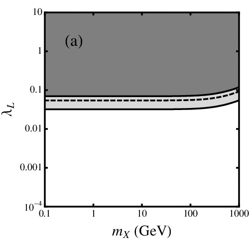
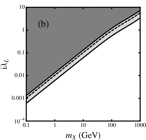
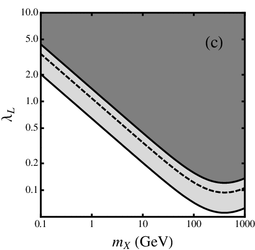
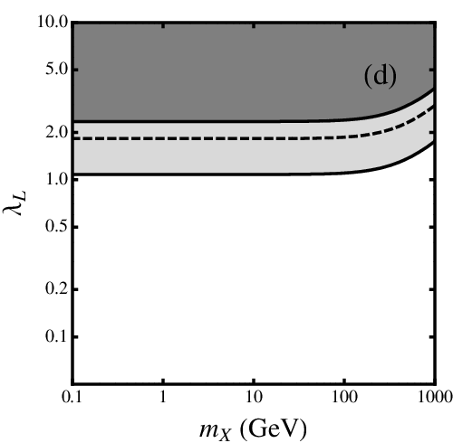
This discrepancy could be lessened if additional sources contribute to the muon’s anomalous magnetic moment, as in the cases above. In Fig. 3 we plot the contribution to aμa_{\mu} in each of the four cases as functions of mXm_{X} while fixing λL=0.1\lambda_{L}=0.1, λR=0\lambda_{R}=0, and mY=400​GeVm_{Y}=400~{\rm GeV} in Cases I and II, and mYL=400​GeVm_{Y_{L}}=400~{\rm GeV} in Cases III and IV. In Case II, we have actually plotted −(Δ​aμ)2-\left(\Delta a_{\mu}\right)_{2}, since, for these parameter choices, it is negative.

Refer to caption
Figure 3: Contributions to aμa_{\mu} as functions of mXm_{X} for λL=0.1\lambda_{L}=0.1, λR=0\lambda_{R}=0, and mY=400​GeVm_{Y}=400~{\rm GeV} in Cases I (solid), II (dashed), III (dotted) and IV (dot-dashed). Note that we have plotted −(Δ​aμ)2-\left(\Delta a_{\mu}\right)_{2} in Case II (dashed) since it is negative for these choices of λL,R\lambda_{L,R}. We use the full one loop expressions for (Δ​aμ)1,…,(Δ​aμ)4\left(\Delta a_{\mu}\right)_{1},\dots,\left(\Delta a_{\mu}\right)_{4}. The light gray band shows values of Δ​aμ\Delta a_{\mu} for which the discrepancy between the theoretical and experimental values of aμa_{\mu} (Eq. 37) is reduced to 1​σ1\sigma.

We see that the helicity flip along the fermion line gives a factor of mXm_{X} in Case III, which suppresses its contributions to aμa_{\mu} at small mXm_{X} for fixed mYLm_{Y_{L}}. For smaller values of mXm_{X}, Case II gives a larger contribution to aμa_{\mu} than in any of the other scenarios. We note that the contributions to aμa_{\mu} for a fermionic XX are generally smaller than for a bosonic XX, given the same value of the coupling.

If any one of these scenarios describes the dominant contribution to the muon’s anomalous magnetic moment beyond the standard model, we can ask what values of λL,R\lambda_{L,R} for a given mXm_{X} and mYm_{Y} reduce the difference between the experimental and theoretical values of aμa_{\mu} to less than 2​σ2\sigma. Fixing λR=0\lambda_{R}=0 and mY=400​GeVm_{Y}=400~{\rm GeV} in Cases I and II, and mYL=400​GeVm_{Y_{L}}=400~{\rm GeV} in Cases III and IV, we plot such values of λL\lambda_{L} as functions of mXm_{X} in Fig. 4.

Refer to caption
Refer to caption
Refer to caption
Refer to caption
Figure 4: Allowed values of λL\lambda_{L} in the situation where XX and YY couple only to μL\mu_{L}, λR=0\lambda_{R}=0, as a function of mXm_{X} for mY=400​GeVm_{Y}=400~{\rm GeV} in Cases I (a) and II (b) and mYL=400​GeVm_{Y_{L}}=400~{\rm GeV} in Cases III (c) and IV (d). In Case II (b), we plot i​λLi\lambda_{L} since a real λL\lambda_{L} would give a negative (Δ​aμ)2\left(\Delta a_{\mu}\right)_{2}. We use the full one loop expressions for (Δ​aμ)1,…,(Δ​aμ)4\left(\Delta a_{\mu}\right)_{1},\dots,\left(\Delta a_{\mu}\right)_{4}. The light gray bands indicate values of λ\lambda and mXm_{X} for which the discrepancy between the theoretical and experimental values of aμa_{\mu} is reduced to less than 2​σ2\sigma. The dashed lines show the values of λ\lambda and mXm_{X} where this discrepancy is 0​σ0\sigma. The dark gray regions contain points where the theoretical value of aμa_{\mu} is at least 2​σ2\sigma larger than the experimental value. The unshaded regions show points where the experimental value of aμa_{\mu} remains at least 2​σ2\sigma larger than the theoretical value.

As we expect from Fig. 3, λ\lambda is constrained to smaller values in Cases I and II than in III and IV. Also, we note that in Case III, the contribution to aμa_{\mu} is proportional to mXm_{X}, which suppresses it for low values of mXm_{X}.

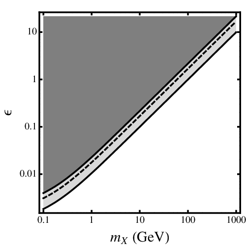
We also show the contribution to aμa_{\mu} as functions of mXm_{X} with λ=ϵ​e=0.06\lambda=\epsilon e=0.06 in Case II with YY identified as the muon in Fig.   5. Also shown are allowed values of ϵ\epsilon as function of mXm_{X}.

Refer to caption
Refer to caption
Figure 5: Left: Contribution to aμa_{\mu} as functions of mXm_{X} for λ=ϵ​e=0.06\lambda=\epsilon e=0.06 or ϵ≃0.2\epsilon\simeq 0.2 in Case II with YY identified as the muon. The light gray band shows values of aμa_{\mu} within the range Δ​aμ±2​σ\Delta a_{\mu}\pm 2\sigma. Right: allowed values of ϵ\epsilon as a function of mXm_{X} in the same case. The light gray bands indicate values of ϵ\epsilon and mXm_{X} for which the discrepancy between the theoretical and experimental values of aμa_{\mu} is less than 2​σ2\sigma. The dark gray regions contain points where the theoretical value of aμa_{\mu} is at least 2​σ2\sigma larger than the experimental value. The unshaded regions show points where the experimental value of aμa_{\mu} remains at least 2​σ2\sigma larger than the theoretical value.

We note that a fermionic XX (Cases III and IV) can be more strongly coupled to muons without violating experimental constraints on aμa_{\mu} if its mass is much smaller than that of YY. If YY’s are observed at the Tevatron or at the LHC, their decay widths can be compared with their contribution to aμa_{\mu} to help determine their spin.

V Conclusions

The experimental value of aμa_{\mu} and its value in the SM currently differ at the 3.1​σ3.1\sigma level. This could be a sign of physics beyond the SM. Hidden sectors that couple to muons can provide an explanation of this deviation. In particular, situations in which the muon is coupled to particles that are charged under both the SM and a hidden symmetry group, GG, and to particles only charged under GG could give rise to a nonzero Δ​aμ\Delta a_{\mu}. These particles could also be found in collider experiments and measurements of their spins and couplings could shed light on the possibility that they contribute significantly to aμa_{\mu}.

The spins of the hidden or mixed particles that couple to the muon greatly affect the structure of their contributions to aμa_{\mu}. In particular, when a fermionic SM singlet is coupled to the muon with a bosonic connector, the constraints on the coupling strength from aμa_{\mu} are less severe for SM singlet masses less that about 100​GeV100~{\rm GeV}. In this way, it is easier to “hide” a light fermionic SM singlet that couples to the muon than a bosonic one.

It is also worth considering whether couplings of the form of Eq. 5, in the case where XX is a dark matter candidate, could be responsible for the recent excesses seen in cosmic ray positrons seen by the PAMELA experiment [14]. Depending on the values of λL\lambda_{L} and λR\lambda_{R}, the dominant annihilation channel for XX’s could be X​X→μ+​μ−XX\to\mu^{+}\mu^{-} through t-channel YY exchange. Dark matter decays into a pair of muons are seen to fit the positron data reasonably well (modulo boost factors) [15], while the muons are kinematically constrained from producing baryons and so would not violate experimental limits on the antiproton fraction of cosmic rays. Future work will study this in more detail.

A proposed muon (g−2)(g-2) experiment hopes to reduce the current experimental error on aμa_{\mu} by a factor ∼4\sim 4 [16]. The uncertainty on the difference between the theoretical and experimental values would then be dominated by the theoretical errors. Such a measurement would help to determine the significance of the deviation between experimental and theoretical values of the muon’s anomalous magnetic moment which is a powerful probe of physics beyond the SM.

Acknowledgements.
The author would like to thank J. L. Rosner, Q.-H. Cao, R. J. Hill, D. Krop, A. M. Thalapillil, and P. Draper for discussions and helpful suggestions. This work was supported in part by the United States Department of Energy under Grant No. DE-FG02-90ER40560.

Appendix A YY Pair Production in e+​e−e^{+}e^{-} Collisions

A.1 Fermionic YY Production Cross Section

For a fermionic YY, we consider the case where its representation under S​U​(2)L×U​(1)YSU(2)_{L}\times U(1)_{Y} is the same as that of the muon. That is, YLY_{L} is a doublet under S​U​(2)LSU(2)_{L} with hypercharge −1-1 while YRY_{R} is an S​U​(2)LSU(2)_{L} singlet with hypercharge −2-2. Its couplings to the photon and ZZ boson are then the same as the muon’s. The Feynman rule for the electron’s (which is the same as the muon’s) coupling to the ZZ boson is shown in Fig. 6.

Refer to caption
Figure 6: Feynman rules for the e+−e−−Ze^{+}-e^{-}-Z vertex (and the μ+−μ−−Z\mu^{+}-\mu^{-}-Z vertex). G=e/(sinθWcosθW)G=e/\left(\sin\theta_{W}\cos\theta_{W}\right), a=1/4−sin2⁡θWa=1/4-\sin^{2}\theta_{W}, and b=1/4b=1/4 with the weak mixing angle sin2⁡θW=0.231\sin^{2}\theta_{W}=0.231.

The cross section, ignoring the width of the ZZ, for e+​e−→Y​Y¯e^{+}e^{-}\to Y\bar{Y} is easily found to be

σ⁡(e+​e−→Y​Y¯)\displaystyle\sigma\left(e^{+}e^{-}\to Y\bar{Y}\right) =2​π​α2sβ{[1+2​G2​a2e2(ss−mZ2)](1−13β2)\displaystyle=\frac{2\pi\alpha^{2}}{s}\beta\left\{\left[1+\frac{2G^{2}a^{2}}{e^{2}}\left(\frac{s}{s-m_{Z}^{2}}\right)\right]\left(1-\frac{1}{3}\beta^{2}\right)\right. (38)
+G4​(a2+b2)e4(ss−mZ2)2(a2−12(a2−b2−13)β2)}\displaystyle\quad\quad\quad\quad\left.+\frac{G^{4}\left(a^{2}+b^{2}\right)}{e^{4}}\left(\frac{s}{s-m_{Z}^{2}}\right)^{2}\left(a^{2}-\frac{1}{2}\left(a^{2}-b^{2}-\frac{1}{3}\right)\beta^{2}\right)\right\} (39)

where GG, aa, and bb, as seen in Fig. 6, are expressed in terms of the electron’s charge and the weak mixing angle θW\theta_{W} as

G\displaystyle G =esinθWcosθW,\displaystyle=\frac{e}{\sin\theta_{W}\cos\theta_{W}}~~~, (40)
a\displaystyle a =14−sin2⁡θW,\displaystyle=\frac{1}{4}-\sin^{2}\theta_{W}~~~, (41)
b\displaystyle b =14.\displaystyle=\frac{1}{4}~~~. (42)

A.2 Scalar YY Production Cross Section

For a scalar YLY_{L} we assume that it couples to the ZZ boson in a gauge invariant way with a strength equal to that of the left-handed muon. We assume analogously for a scalar YRY_{R}. The Feynman rules for these YL−YR−γY_{L}-Y_{R}-\gamma and YL−YR−ZY_{L}-Y_{R}-Z couplings are shown in Fig. 7.

Refer to caption
Refer to caption
Figure 7: Feynman rules for a scalar YY. All momenta are running into the graphs. We use ZLS=e(1−2sin2θW)/(2sinθWcosθW)Z^{S}_{L}=e\left(1-2\sin^{2}\theta_{W}\right)/\left(2\sin\theta_{W}\cos\theta_{W}\right) and ZSR=−etanθWZ^{S}_{R}=-e\tan\theta_{W}.

We then obtain

σ⁡(e+​e−→YL,R+​YL,R−)=π​α2s​(β33)​{1+2​G​ae2​ZL,RS​(ss−mZ2)+G2​(a2+b2)e4​(ZL,RS)2​(ss−mZ2)2}\displaystyle\sigma\left(e^{+}e^{-}\to Y_{L,R}^{+}Y_{L,R}^{-}\right)=\frac{\pi\alpha^{2}}{s}\left(\frac{\beta^{3}}{3}\right)\left\{1+\frac{2Ga}{e^{2}}Z_{L,R}^{S}\left(\frac{s}{s-m_{Z}^{2}}\right)+\frac{G^{2}\left(a^{2}+b^{2}\right)}{e^{4}}\left(Z_{L,R}^{S}\right)^{2}\left(\frac{s}{s-m_{Z}^{2}}\right)^{2}\right\} (43)

where we have again ignored the width of the ZZ. GG, aa, and bb are as in Eqs. 40-42 and

ZLS\displaystyle Z^{S}_{L} =e⁡(1−2​sin2⁡θW)2sinθWcosθW,\displaystyle=\frac{e\left(1-2\sin^{2}\theta_{W}\right)}{2\sin\theta_{W}\cos\theta_{W}}~~~, (44)
ZRS\displaystyle Z^{S}_{R} =−etanθW.\displaystyle=-e\tan\theta_{W}~~~. (45)

A.3 Vector YY Production Cross Section

To properly determine the cross section for vector YY pair production we need to introduce new states to insure unitarity is not violated. As mentioned in Sec. II, we assume that there is an electrically neutral fermion that couples to YL,RνY_{L,R}^{\nu} and eL,Re_{L,R} which we call NL,RN_{L,R}. We write the Feynman rules for the interactions of YL,RνY_{L,R}^{\nu} with e±e^{\pm}, ZZ, and NL,RN_{L,R} in Fig. 8. The coupling strengths gLg_{L} and ZL,RVZ_{L,R}^{V} will be chosen so that the cross section for e+​e−→YLν+​YLν−e^{+}e^{-}\to Y_{L}^{\nu+}Y_{L}^{\nu-} remains finite as s→∞\sqrt{s}\to\infty.

Refer to caption
Refer to caption
Refer to caption
Figure 8: Feynman rules for a vector YY. Vμ​ν​ρ​(p,k,q)=[(p−k)ρ​gμ​ν+(k−q)μ​gν​ρ+(q−p)ν​gμ​ρ]V^{\mu\nu\rho}\left(p,k,q\right)=\left[\left(p-k\right)^{\rho}g^{\mu\nu}+\left(k-q\right)^{\mu}g^{\nu\rho}+\left(q-p\right)^{\nu}g^{\mu\rho}\right] and all momenta are running into the graphs. The photon interaction is fixed by demanding electromagnetic gauge invariance. The values of gLg_{L} and ZL,RVZ_{L,R}^{V} are determined by requiring that they that keep YY pair production unitary. They are given in Eq. 60.

We write the cross section for the production of pair of vector YLY_{L}s as

d​σd​cos⁡θ​(e+​e−→YLν+​YLν−)=π​α216​βs​∑|ℳi​j|2\displaystyle\frac{d\sigma}{d\cos\theta}\left(e^{+}e^{-}\to Y_{L}^{\nu+}Y_{L}^{\nu-}\right)=\frac{\pi\alpha^{2}}{16}\frac{\beta}{s}\sum\left|{\cal M}_{ij}\right|^{2} (46)

where θ\theta is the center-of-mass scattering angle. The squared matrix elements are

|ℳN​N|2\displaystyle\left|{\cal M}_{NN}\right|^{2} =4​gL4e4​(tt−mNL2)2​Ft​(t,s),\displaystyle=\frac{4g_{L}^{4}}{e^{4}}\left(\frac{t}{t-m_{N_{L}}^{2}}\right)^{2}F_{t}\left(t,s\right)~~~, (47)
|ℳγ​γ|2\displaystyle\left|{\cal M}_{\gamma\gamma}\right|^{2} =Fs​(t,s),\displaystyle=F_{s}\left(t,s\right)~~~, (48)
|ℳZ​Z|2\displaystyle\left|{\cal M}_{ZZ}\right|^{2} =G2​(a2+b2)​|ZLV|2e4​(ss−mZ2)2​Fs​(t,s),\displaystyle=\frac{G^{2}\left(a^{2}+b^{2}\right)\left|Z_{L}^{V}\right|^{2}}{e^{4}}\left(\frac{s}{s-m_{Z}^{2}}\right)^{2}F_{s}\left(t,s\right)~~~, (49)
|ℳZ​γ|2\displaystyle\left|{\cal M}_{Z\gamma}\right|^{2} =2​G​a​Re​(ZLV)e2​(ss−mZ2)​Fs​(t,s),\displaystyle=\frac{2Ga~{\rm Re}(Z_{L}^{V})}{e^{2}}\left(\frac{s}{s-m_{Z}^{2}}\right)F_{s}\left(t,s\right)~~~, (50)
|ℳN​Z|2\displaystyle\left|{\cal M}_{NZ}\right|^{2} =−2​G​(a+b)​Re​(ZLV)​gL2e4​(ss−mZ2)​(tt−mNL2)​Fs​t​(t,s),\displaystyle=-\frac{2G\left(a+b\right){\rm Re}(Z_{L}^{V})g_{L}^{2}}{e^{4}}\left(\frac{s}{s-m_{Z}^{2}}\right)\left(\frac{t}{t-m_{N_{L}}^{2}}\right)F_{st}\left(t,s\right)~~~, (51)
|ℳN​γ|2\displaystyle\left|{\cal M}_{N\gamma}\right|^{2} =−2​gL2e2​(tt−mNL2)​Fs​t​(t,s),\displaystyle=-\frac{2g_{L}^{2}}{e^{2}}\left(\frac{t}{t-m_{N_{L}}^{2}}\right)F_{st}\left(t,s\right)~~~, (52)

where ss and tt are the usual Mandelstam variables and we have defined the functions

Ft​(t,s)\displaystyle F_{t}\left(t,s\right) =2​(smYL2)+12​β2​sin2⁡[θ⁡(t)]​[(st)2+14​(smYL2)2],\displaystyle=2\left(\frac{s}{m_{Y_{L}}^{2}}\right)+\frac{1}{2}\beta^{2}\sin^{2}\left[\theta\left(t\right)\right]\left[\left(\frac{s}{t}\right)^{2}+\frac{1}{4}\left(\frac{s}{m_{Y_{L}}^{2}}\right)^{2}\right]~~~, (53)
Fs​(t,s)\displaystyle F_{s}\left(t,s\right) =β2​{16​(smYL2)+sin2⁡[θ⁡(t)]​[(smYL2)2−4​(smYL2)+12]},\displaystyle=\beta^{2}\left\{16\left(\frac{s}{m_{Y_{L}}^{2}}\right)+\sin^{2}\left[\theta\left(t\right)\right]\left[\left(\frac{s}{m_{Y_{L}}^{2}}\right)^{2}-4\left(\frac{s}{m_{Y_{L}}^{2}}\right)+12\right]\right\}~~~, (54)
Fs​t​(t,s)\displaystyle F_{st}\left(t,s\right) =16​(1+mYL2t)+8​β2​(smYL2)+12​β2​sin2⁡[θ⁡(t)]​[(smYL2)2−2​(smYL2)−4​(st)].\displaystyle=16\left(1+\frac{m_{Y_{L}}^{2}}{t}\right)+8\beta^{2}\left(\frac{s}{m_{Y_{L}}^{2}}\right)+\frac{1}{2}\beta^{2}\sin^{2}\left[\theta\left(t\right)\right]\left[\left(\frac{s}{m_{Y_{L}}^{2}}\right)^{2}-2\left(\frac{s}{m_{Y_{L}}^{2}}\right)-4\left(\frac{s}{t}\right)\right]~~~. (55)

We relate θ\theta and tt through

sin2⁡[θ⁡(t)]=−4β2​[(t−mYL2s)2+ts].\displaystyle\sin^{2}\left[\theta\left(t\right)\right]=-\frac{4}{\beta^{2}}\left[\left(\frac{t-m_{Y_{L}}^{2}}{s}\right)^{2}+\frac{t}{s}\right]~~~. (57)

Unitarity will determine the values of gLg_{L} and ZLVZ^{V}_{L}. Requiring that the coefficients of (s/mYL2)2​sin2⁡θ(s/m_{Y_{L}}^{2})^{2}\sin^{2}\theta and of (s/mYL2)(s/m_{Y_{L}}^{2}) vanish as s→∞\sqrt{s}\to\infty gives

gL4+2​[e4+G2​(a2+b2)​|ZLV|2+2​e2​G​a​Re​(ZLV)]−2​gL2​[G⁡(a+b)​Re​(ZLV)+e2]=0,\displaystyle g_{L}^{4}+2\left[e^{4}+G^{2}\left(a^{2}+b^{2}\right)\left|Z_{L}^{V}\right|^{2}+2e^{2}Ga~{\rm Re}(Z_{L}^{V})\right]-2g_{L}^{2}\left[G\left(a+b\right){\rm Re}(Z_{L}^{V})+e^{2}\right]=0~~~, (58)

while setting the coefficient of (s/mYL2)​sin2⁡θ(s/m_{Y_{L}}^{2})\sin^{2}\theta to zero as s→∞\sqrt{s}\to\infty implies

2​[e4+G2​(a2+b2)​|ZLV|2+2​e2​G​a​Re​(ZLV)]−gL2​[G⁡(a+b)​Re​(ZLV)+e2]=0.\displaystyle 2\left[e^{4}+G^{2}\left(a^{2}+b^{2}\right)\left|Z_{L}^{V}\right|^{2}+2e^{2}Ga~{\rm Re}(Z_{L}^{V})\right]-g_{L}^{2}\left[G\left(a+b\right){\rm Re}(Z_{L}^{V})+e^{2}\right]=0~~~. (59)

These two equations are satisfied by

gL2=2​e2​bb−a,ZLV=e2G⁡(b−a).\displaystyle g_{L}^{2}=\frac{2e^{2}b}{b-a}~~~,~~~Z_{L}^{V}=\frac{e^{2}}{G\left(b-a\right)}~~~. (60)

We note that the contribution due to ZZ boson exchange cannot by itself cancel that from photon exchange unless the ZZ coupling to electrons is vector-like (which it is not). These conditions allow us to determine σ⁡(e+​e−→YLν+​YLν−)\sigma\left(e^{+}e^{-}\to Y_{L}^{\nu+}Y_{L}^{\nu-}\right) as a function of mYLm_{Y_{L}} and mNLm_{N_{L}}.

σ⁡(e+​e−→YRν+​YRν−)\sigma\left(e^{+}e^{-}\to Y_{R}^{\nu+}Y_{R}^{\nu-}\right) is obtained from σ⁡(e+​e−→YLν+​YLν−)\sigma\left(e^{+}e^{-}\to Y_{L}^{\nu+}Y_{L}^{\nu-}\right) by taking b→−bb\to-b.

References

  • [1] M. Davier, A. Hoecker, B. Malaescu, C. Z. Yuan and Z. Zhang, arXiv:0908.4300 [hep-ph].
  • [2] J. Prades, E. de Rafael and A. Vainshtein, arXiv:0901.0306 [hep-ph].
  • [3] G. W. Bennett et al. [Muon G-2 Collaboration], Phys. Rev. D 73, 072003 (2006) [arXiv:hep-ex/0602035].
  • [4] J. Prades, arXiv:0909.2546 [hep-ph]; F. Jegerlehner and A. Nyffeler, Phys. Rept. 477, 1 (2009) [arXiv:0902.3360 [hep-ph]]; M. Passera, W. J. Marciano and A. Sirlin, AIP Conf. Proc. 1078, 378 (2009) [arXiv:0809.4062 [hep-ph]].
  • [5] F. Domingo and U. Ellwanger, JHEP 0807, 079 (2008) [arXiv:0806.0733 [hep-ph]]; D. Stockinger, arXiv:0710.2429 [hep-ph].
  • [6] T. Appelquist and B. A. Dobrescu, Phys. Lett. B 516, 85 (2001) [arXiv:hep-ph/0106140].
  • [7] J. A. Conley and J. S. Gainer, arXiv:0811.4168 [hep-ph].
  • [8] B. Holdom, Phys. Lett. B 166, 196 (1986); P. Fayet, Nucl. Phys. B 347, 743 (1990). N. Arkani-Hamed and N. Weiner, JHEP 0812, 104 (2008) [arXiv:0810.0714 [hep-ph]]; C. Cheung, J. T. Ruderman, L. T. Wang and I. Yavin, Phys. Rev. D 80, 035008 (2009) [arXiv:0902.3246 [hep-ph]]; A. Katz and R. Sundrum, JHEP 0906, 003 (2009) [arXiv:0902.3271 [hep-ph]]; D. E. Morrissey, D. Poland and K. M. Zurek, JHEP 0907, 050 (2009) [arXiv:0904.2567 [hep-ph]].
  • [9] M. Pospelov, Phys. Rev. D 80, 095002 (2009) [arXiv:0811.1030 [hep-ph]].
  • [10] J. L. Feng and J. Kumar, Phys. Rev. Lett. 101, 231301 (2008) [arXiv:0803.4196 [hep-ph]]; J. L. Feng, H. Tu and H. B. Yu, JCAP 0810, 043 (2008) [arXiv:0808.2318 [hep-ph]].
  • [11] J. L. Feng, J. Kumar and L. E. Strigari, Phys. Lett. B 670, 37 (2008) [arXiv:0806.3746 [hep-ph]].
  • [12] D. McKeen, Phys. Rev. D 79, 114001 (2009) [arXiv:0903.4982 [hep-ph]].
  • [13] A. Heister et al. [ALEPH Collaboration], Phys. Lett. B 583, 247 (2004); J. Abdallah et al. [DELPHI Collaboration], Eur. Phys. J. C 31, 421 (2003) [arXiv:hep-ex/0311019]; P. Achard et al. [L3 Collaboration], Phys. Lett. B 580, 37 (2004) [arXiv:hep-ex/0310007]; G. Abbiendi et al. [OPAL Collaboration], Eur. Phys. J. C 32, 453 (2004) [arXiv:hep-ex/0309014].
  • [14] O. Adriani et al. [PAMELA Collaboration], Nature 458, 607 (2009) [arXiv:0810.4995 [astro-ph]].
  • [15] P. Meade, M. Papucci, A. Strumia and T. Volansky, arXiv:0905.0480 [hep-ph].
  • [16] D. W. Hertzog, Nucl. Phys. Proc. Suppl. 181-182, 5 (2008); R. M. Carey et al., “The New (g-2) Experiment: A proposal to measure the muon anomalous magnetic moment to +-0.14 ppm precision”; K. R. Lynch [Muon (g-2) Collaboration], Nucl. Phys. Proc. Suppl. 189, 201 (2009).