Exact solutions of the modified Gross-Pitaevskii equation in ‘smart’ periodic potentials in the presence of external source
Abstract
We report wide class of exact solutions of the modified Gross-Pitaevskii equation (GPE) in ‘smart’ Jacobi elliptic potentials: , , and in the presence of external source. Solitonlike solutions, singular solutions, and periodic solutions are found using a recently developed fractional transform: , where is the respective Jacobi elliptic function and the amplitude parameters , , and nonzero. These results generalize those contained in (Paul T, Richter K and Schlagheck P 2005 Phys. Rev. Lett. 94, 020404) for nonzero trapping potential.
1 Introduction
In a mean-field approximation, the dynamics of a dilute-gas Bose-Einstein condensate (BEC) can be captured by the cubic nonlinear Schrödinger equation (NLSE) with a trapping potential [1, 2, 3]. The various traps which are used to contain the BEC have spurred the solutions of the NLSE with new potentials [4, 5]. We consider the mean-field model of a quasi-one-dimensional BEC trapped in a ‘smart’ potential in the presence of an external source[6]
| (1) |
where represents the macroscopic wave function of the condensate and is an experimentally generated macroscopic potential. The parameter indicates the strength of atom-atom interactions and it alone decides whether Eq. (1) is attractive (, focussing nonlinearity) or repulsive (, defocussing nonlinearity). Here, and are real constants related to the source amplitude and the chemical potential, respectively, and is a real function of , and being two real parameters. In the field of nonlinear optics, Eq. (1) may describe the evolution of the local amplitude of an electromagnetic wave in the spatial domain, in a two-dimensional waveguide where becomes the propagation distance and becomes the retarded time, and the system is driven by an external plane pump wave. The Jacobi elliptic potential may describe a transverse modulation of the refractive index in the waveguide.
As is well-known, Eq. (1) is not integrable if , and only small classes of explicit solutions can most likely exist. For , Eq. (1) is a cubic NLSE with a source, and exact rational solutions using a fractional transform are found in Ref. [7]. And in Ref. [11] periodic solutions without source have been reported. More recently, in Ref.[8], a class of exact solutions of Eq. (1) for have been reported. In particular, the rational solutions of the fractional transform: , where have been reported for . This is due to the form of the trapping potential. Nonetheless, in the present paper we find rational solutions of the type , where being the respective Jacobi elliptic function with all the amplitude parameters , , and nonzero. These results generalize those contained in Ref [6] for nonzero trapping potential. The choice of a smart potential allows one to construct a large class of exact solutions, as done in a number of works for the cubic GP equations [9, 10, 11]. In the present work, we consider three different potentials in the GP equation: , , and in the presence of external source, and find exact travelling wave solutions of Eq. (1) with . The choice of these three different ‘smart’ potentials is motivated by the following facts. Firstly, the potential in the limit is which is similar to the standard optical lattice potential [12, 13]. Secondly, the choice of the potential in GP equation mimics[14] the harmonic potential that was used to achieve BEC experimentally. The third potential, we hope it is relevant to the available experimental conditions to achieve BEC.
2 EXACT SOLUTIONS OF THE GPE IN ‘SMART’ PERIODIC POTENTIAL WITH SOURCE
The travelling wave solutions of Eq. (1) with potential are taken to be of the form . Inserting this expression for in Eq. (1) and separating the real and imaginary parts, and integrating the imaginary part, one gets
| (2) |
where is a constant of integration. In order that the external phase be independent of , we consider only solutions with , to obtain
| (3) |
Below we consider three different ‘smart’
Jacobi elliptic potentials [15] and find exact solutions.
Case(I):- . Eq. (3) reads
as
| (4) |
Substituting
| (5) |
in Eq.(4) and equating the coefficients of equal powers of result in relations among the solution parameters , and , and the equation parameters , , , , and . We find that
| (6) | |||
| (7) |
From Eq. (7) it follows that and implying the GPE with repulsive nonlinearity.
Case(II):- . Eq. (3) reads as
| (8) |
Substituting
| (9) |
in Eq.(8) and equating the coefficients of equal powers of result in relations among the solution parameters , and , and the equation parameters , , , , and . We find that
| (10) | |||
| (11) |
From the positivity of we conclude that solutions exist for and . The condition corresponds to the GPE with attractive nonlinearity.
Case(III):- . Eq. (3) reads as
| (12) |
Substituting
| (13) |
in Eq.(12) and equating the coefficients of equal powers of result in relations among the solution parameters , and , and the equation parameters , , , , and . We find that
| (14) | |||
| (15) |
Here we conclude that solutions exist only for and .
3 Rational solutions
In order to obtain Lorentzian-type of solutions of Eq. (3) we use a fractional transform
| (16) |
where is the respective Jacobi elliptic functions. Again we
obtain the Lorentzian-type of solutions of Eq. (3) for three
different ‘smart’ potentials.
Case(I):-. Eq. (3) reads
as
| (17) |
Substituting
| (18) |
in Eq.(17) and equating the coefficients of equal powers of will yield the following consistency conditions.
| (19) | |||
| (20) | |||
| (21) | |||
| (22) | |||
| (23) | |||
| (24) | |||
| (25) |
From the above consistency conditions we obtain the following relations.
| (26) | |||
| (27) |
where . Here, we would like to emphasize that these results generalize those contained in Ref [6], for nonzero trapping potential. This stems from the fact that the constant in expression (18) is nonzero, which follows from the choice of our ‘smart’ potential in Eq. (1).
Case(II):-. Eq. (3) reads as
| (28) |
Substituting
| (29) |
in Eq.(28) and equating the coefficients of equal powers of will yield the following consistency conditions.
| (30) | |||
| (31) | |||
| (32) | |||
| (33) | |||
| (34) | |||
| (35) | |||
| (36) |
From the above consistency conditions we obtain the following relations
| (37) | |||
| (38) |
Case(III):- . Eq. (3) reads as
| (39) |
Substituting
| (40) |
in Eq.(39) and equating the coefficients of equal powers of will yield the following consistency conditions.
| (41) | |||
| (42) | |||
| (43) | |||
| (44) | |||
| (45) | |||
| (46) | |||
| (47) |
From the above consistency conditions we obtain the following relations
| (48) | |||
| (49) |
3.1 Trigonometric solutions
From the consistency conditions that arise from the first two ‘smart’ periodic potentials, we conclude that the limit is forbidden as the amplitude parameters , , and will be zero. On the other hand, for case, only flat background solutions will be possible for limit.
3.2 Solitonlike solutions
Here, in this subsection, we describe the solitonlike solutions that are obtained from the solutions in and in the limit , in detail. In the limit , becomes an array of well separated kink-type of potential barriers: . Then we have the following relations
| (50) | |||
| (51) |
And the strength of the source is
As a special case, if we set and , then we get , , and . This results in a solitonlike solution
| (52) |
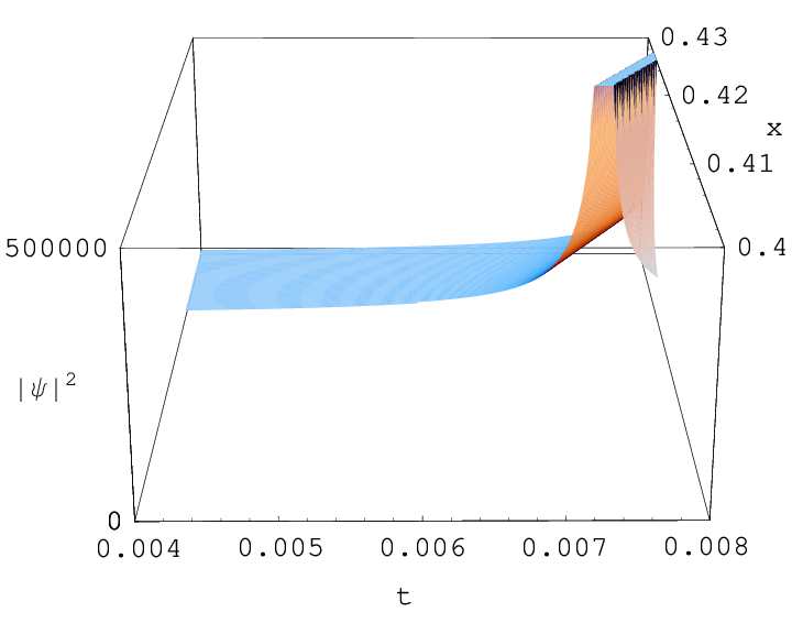
This set corresponds to the singular solution for repulsive case i.e., . The singularity of the pulse profile may correspond to the beam power exceeding material breakdown due to self-focussing [16, 17, 18, 19]. Figure (1) depicts a surface plot of this solution for the parameter values given in the figure caption.
Another interesting solitonlike solution is obtained from the solution in for . In the limit , becomes an array of well separated secant hyperbolic potential barriers: .Then we have the following relations
| (53) | |||
| (54) |
As a special case, if we set , , and then we get , , and . This results in a solitonlike solution
| (55) |
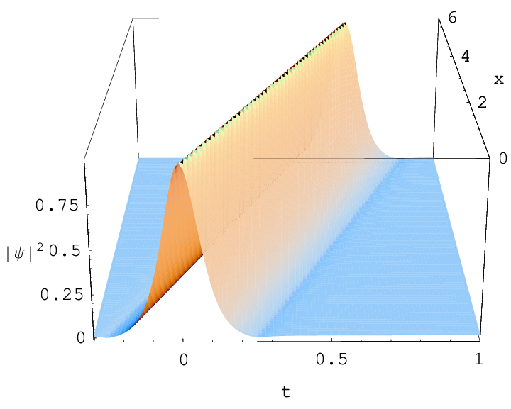
This set corresponds to the non-singular solution for attractive case i.e., . The same has been depicted in Fig. 2 for the parameter values given in in the figure caption.
4 Conclusions
In conclusion, we have shown the existence of wide class of exact solutions for the modified GP equation in ‘smart’ periodic potentials with an external source. The Lorentzian-type of solitons are obtained with the aid of a fractional transform. Our analysis applies to both attractive and repulsive cases of GP equation. Furthermore, our rational solutions generalize those contained in Ref [6], for nonzero trapping potential, because of our choice of ‘smart’ potential. We hope that these potentials may be experimentally realizable, to achieve BEC. Although not presented here, the stability of these wide class of solutions can be checked using a semi-implicit Crank-Nicholson finite difference method [7], as the much used numerical techniques based on fast Fourier transform (FFT) requires the FFT of the source, which is costly.
Acknowledgements
TSR would like to dedicate this paper to the fond memory of his father Shri. Thokala Ratna Raju, for his love and encouragement.
References
References
- [1] Dalfovo F, Giorgini S, Pitaevskii L P and Stringari S 1999 Rev. Mod. Phys. 71, 463
- [2] Carr L D, Leung M A and Reinhardt W P 2000 J. Phys. B: At. Mol. Opt. Phys. 33, 3983 and references therein
- [3] Bongs K et al., 2001 Phys. Rev. A 63, 031602
- [4] Kunze Met al., 1999 Physica D 128, 273; Kivshar Y S, Alexander T J and Turitsyn S K 2001 Phys. Lett. A 278, 225
- [5] Carr L D, Clark C W and Reinhardt W P 2000 Phys. Rev. A 62, 063610; Carr L D, Clark C W and Reinhardt W P 2000 Phys. Rev. A62, 063611
- [6] Paul T, Richter K and Schlagheck P 2005 Phys. Rev. Lett. 94, 020404
- [7] Soloman Raju T, Nagaraja Kumar C and Panigrahi P K 2005 J. Phys. A: Math. and Gen. 38, L271
- [8] Kengne E and Vaillancourt R 2007 J. Math. Phys. 48, 073520
- [9] Bronski J C, Carr L D, Deconinck B and Kutz J N 2001 Phys. Rev. Lett. 86, 1402
- [10] Bronski J C, Carr L D, Deconinck B, Kutz J N and Promislow K 2001 Phys. Rev. E 63, 036612
- [11] Bronski J C, Carr L D, Carretero-González R, Deconinck B, Kutz J N and Promislow K 2001 Phys. Rev. E 64, 056615
- [12] Choi D I and Niu Q 1999 Phys. Rev. Lett. 82, 2022
- [13] Berg-Sorensen K and Mlmer K 1998 Phys. Rev. A 58, 1480
- [14] Kengne E, Vaillancourt R and Malomed B A 2008 J. Phys. B: At. Mol. Opt. Phys. 41, 205202 and references therein
- [15] Abramowitz M and Stegun I A 1964 Handbook of Mathematical Functions(Washington, DC, National Bureau of Standards)
- [16] Fibich G and Gaeta A L 2000 Opt. Lett. 25, 335
- [17] Mollenauer L F, Stolen R H and Gordon J P 1980 Phys. Rev. Lett. 45, 1095
- [18] Boyd R W 1992 Nonlinear Optics(Academic Press, Boston, MA)
- [19] Weinstein M 1983 Commun. Math. Phys. 87, 567