Approximate reconstruction of bandlimited functions for the integrate and fire sampler
Abstract.
In this paper we study the reconstruction of a bandlimited signal from samples generated by the integrate and fire model. This sampler allows us to trade complexity in the reconstruction algorithms for simple hardware implementations, and is specially convenient in situations where the sampling device is limited in terms of power, area and bandwidth.
Although perfect reconstruction for this sampler is impossible, we give a general approximate reconstruction procedure and bound the corresponding error. We also show the performance of the proposed algorithm through numerical simulations.
Key words and phrases:
Keywords: integrate and fire, non-uniform sampling, bandlimited function.1. Introduction
The integrate and fire (IF) model is well known in computational neuroscience as a simplified model of a neuron [8, 12] and is typically used to study the dynamics of large populations. The model consists of a leaky integrator followed by a comparator. The leak corresponds to a gradual loss of the value of the integral.
More recently, the IF model has also been considered as a sampler [4, 16, 10, 11], where the sampler output is tuned to the variation of the integral of the signal. This feature can be exploited when sampling neural recordings, for which relevant information is localized in small intervals where the signal has a high amplitude [3].
The block diagram of the sampler is presented in Figure 1. At every instant , the continuous input is integrated against an averaging function and the result is compared to a positive and negative threshold. When either of these is reached, a pulse is created at time representing the threshold value (positive or negative), the value of the integrator is then reset and the process repeats.

The output is a nonuniformly spaced pulse train, where each of the pulses is either 1 or -1. The averaging function is defined by , where is the characteristic function of and is a constant that models the leakage of the integrator due to practical implementations. The precise firing condition determining the pulses is:
| (1) |
The simplicity of the sampler translates into an efficient hardware implementation which saves both power and area when compared to conventional analog-to-digital converters (ADC) [4]. These constraints are severe, in the case of wireless brain machine interfaces [13], for which the entire system has to be embedded inside the subject. Hence, the IF sampler allows us to move the complexity of the design into the reconstruction algorithm while providing a simple front end at the sampling stage.
The problem of reconstructing a signal from the IF output should be distinguished from the study of the dynamics of a population of neurons, when some stochastic assumption is made on the firing parameters [9]. In this article we study the deterministic reconstruction of a bandlimited signal from the integrate and fire output. Part of the challenge of this stems from the fact that the sampling map that associates a function to its samples is non-linear. Indeed, we see from Equation (1) that the magnitude of the samples is always . Moreover, exact reconstruction for the IF sampler is impossible since the output of the sampler does not completely determine the signal (see Example 1 below.)
In this article, we will show that it is however possible to approximately reconstruct a bandlimited signal in norm with an error comparable to the threshold . Moreover, we give a concrete reconstruction procedure which is of course non-linear but, nevertheless, easy to implement. Since in many situations the IF sampler is so much more convenient to implement than conventional analog-to-digital converters, the loss of accuracy in the reconstruction is a very reasonable trade-off [4], specially if the final analysis of the reconstructed data tolerates some small error [3].
The methods considered so far [11] reconstruct the signal from the system of equations (cf. Equation (1)), thus treating the reconstruction as a (linear) average sampling problem (see [7, 1, 15, 14]). These approaches impose density restrictions on the set of sampling functions (cf. Equation (1).) Since these sampling functions depend on the signal, the density constraints on them are somehow unnatural.
The key for the reconstruction method that we develop lies in the observation that the information derived from the IF output is much richer than the mere system of equations . It also contains the information that no proper subinterval of satisfies Equation (1). We will exploit this extra information to give an approximate reconstruction procedure for a general bandlimited function. Since the sampling process starts at a certain instant , an additional assumption on the size of before is required in order to fully reconstruct . Roughly speaking, the assumption means that the sampling scheme would not have produced any pulse before .
In Section 2 we formally describe the output of the IF sampling scheme. This output depends on an initial time when the process is started and two parameters: the threshold and the constant modeling the leakage on the sampler. In Section 1 we show that the IF output is always a finite sequence. Section 4 gives the approximate reconstruction procedure and Section 5 presents some numerical experiments.
2. The integrate and fire sampling problem
We now define precisely the integrate and fire sampling scheme. Throughout the article we will assume the following.
Assumption 1.
A bandlimited function and numbers , are given.
Here, is the Paley-Wiener space
of (complex-valued) bandlimited functions and is the Fourier transform of . We call the initial time, the firing parameter and the threshold. Using these parameters we formally define the output of the sampler. We first define recursively a finite or countable sequence called the time instants. Suppose that the instants have already been defined and consider the function given by
Observe that is continuous and . If , for all , then the process stops. If , for some , by the continuity of , we can define as the minimum number satisfying the equation
| (2) |
Clearly, in this case .
We have defined a finite or countable sequence of points . We will prove in Proposition 1 that this sequence is in fact finite. Let us assume the time instants and define the samples by,
| (3) |
Observe that, by the definition of the time intervals, .
The output of the sampler is formally given by the time instants and the numbers . We say that this output has been produced by the integrate and fire. The succeeding results apply generally to complex-valued functions, but in the case of the application that motivated this sampling scheme, the signal is taken to be real-valued, and the output of the sampler is encoded as a train of impulses, where only the sign of the samples is stored.
3. Some remarks on the IF output
First we note that bandlimited functions are not completely determined by the output of the IF sampler.
Example 1.
There are non-zero bandlimited signals that will never produce an output from the sampler. Take for instance . Since , is bandlimited. We have for any , for all
We now prove that the set of time instants produced by the IF sampler is indeed finite and give some bounds on its distribution. To this end we introduce some auxiliary functions that will be used throughout the remainder of the article.
Consider the function given by and define,
| (4) |
Since , . In the Fourier domain, and are related by
| (5) |
In the time domain, this can be expressed as
| (6) |
Observation 1.
The function is continuous and , when .
Proof.
We have already observed that . Since and , we have that and the conclusion follows from the Riemann-Lebesgue Lemma. ∎
The following straightforward equation relates to the integrate and fire process.
| (7) |
We can now prove that the output of the IF process is finite.
Proposition 1.
Under Assumption 1, the following holds.
- (a)
The set of time instants produced by the integrate and fire scheme is a finite set .
- (b)
The numbers of time instants in a given finite interval is bounded by
- (c)
If is integrable, the total number of time instants is bounded by
Proof.
We first prove (b) and (c). Let be an interval and let be consecutive time instants contained in . If the bound is trivial, so assume that . For each , using Equation (2) we have,
Summing over the intervals determined by the points we have,
| (8) |
Letting and yields (b). For (a), Hölder’s inequality gives,
and the conclusion follows.
4. The reconstruction
We now address the problem of approximately reconstructing a bandlimited function from the integrate and fire output. Since the samples are taken in the half-line we will make some assumption about the size of before the initial instant. Roughly speaking, the integrate and fire process would not have produced any sample in the interval .
Assumption 2.
The function defined in Equation (4) satisfies,
Note that by Observation 1, any satisfies this assumption. To approximately reconstruct we will first approximately reconstruct from the integrate and fire output and then derive information about by means of Equation (5). We will use the structure of the IF process to produce a number of approximate samples for .
First we argue that, from the output of the IF process, we have enough information to approximate on the time instants . Rewriting Equation (3) in terms of (cf. Equation (7)) we have,
| (9) |
Since the value may not be exactly known we cannot determine from this recurrence relation all the values . However, we can construct an approximation to these values. Let and define recursively,
| (10) |
Observe that Assumption 2 implies that . Using this estimate as a starting point we can iterate on Equation (9) and (10) to get,
| (11) |
Consequently, using only the output of the IF sampling scheme, we have constructed a set of values that approximates on the instants . The second step is to approximate on an arbitrary point of .
To this end observe that, according to the definition of as the minimum number satisfying Equation (2), we have that,
Rewriting this inequality in terms of (cf. Equation (7)) gives,
| (12) |
Combining this last inequality with (11) yields,
| (13) |
We now show that this inequality allows us to approximate anywhere on the line.
Claim 1.
Given an arbitrary time instant , choose in the following way:
- (a)
if , let ,
- (b)
if belongs to some (unique) interval , let ,
- (c)
if , let .
Then, .
Remark 1.
Observe that the procedure to obtain from depends only on the output of the IF process.
Proof.
We will now choose a window function.
Assumption 3.
A Schwartz class function such that
- •
on , and,
- •
is compactly supported,
has been chosen.
Since , the classic oversampling trick for bandlimited functions (see for example [6] or [7]) implies that there exists a number such that
| (15) |
Using the procedure described in Claim 1, we produce a set such that
| (16) |
Let be the function defined by,
| (17) |
It follows that is also a Schwartz function. Moreover, using Equation (5) we have that,
| (18) |
Observe that, since , the sequence and the series in Equation (18) converges in and uniformly - in fact, it converges in the Wiener amalgam norm , see for example [6], [7] and [2].)
Now we can define the approximation of constructed from the IF samples. Let,
| (19) |
Since, by Inequality (16), the sequence is bounded and is a Schwartz function, it follows that Equation (19) defines a bounded function and that the convergence is uniform (see [6] or [2].)
The reconstruction algorithm consists then of calculating the approximated samples following Claim 1 and then convolving them with the kernel , that can be pre-calculated.
We now give a precise error bound for the reconstruction.
Theorem 1.
Proof.
Remark 2.
We currently do not know what choice of the window function minimizes the constant in the theorem. A more detailed study of the choice of the window function should not only consider the size of that constant but also the rate of convergence of the series in Equation (19).
5. Numerical experiments
We study the behavior of the reconstruction algorithm under variations in the threshold and the oversampling period for a specific choice of reconstruction kernel . The test signal is of finite length and real valued, produced as a linear combination of five ‘sinc’ kernels () at a 1Hz frequency, with random locations and weights. The amplitude of the input has been normalized to 1. Although the theory covers infinite dimensional spaces, our simulations are limited by the practical implementations of the sampler and algorithms. The effects of truncation and quantization are not considered here.
This signal is encoded by the IF sampler with and recovered using the procedure described in Section 4. The reconstruction kernel is a raised cosine, defined by,
| (20) |
where and are determined by the maximum input frequency and the desired oversampling period (cf. Equation (15).) Figure 2(a) shows the raised cosine in the time and frequency domain. Observe that the spectrum of is constant for frequencies less than the input bandwidth and then decays smoothly towards zero. The corresponding kernel (cf. Equation (17)) is shown in Figure 2(b).


Using we recover (cf. Equation (19).), an approximation of as shown in Figure 3. As expected the error decreases in regions with high density of samples. This behavior is evident from Figure 4, the dense regions imply that the uniform samples will most likely coincide with the estimated values of at the sample locations. On the other hand, for samples that are far apart the approximation follows a exponential decay from its original value which is not the natural trend in the signal. Figure 4 shows (solid line), and the approximated samples of on the lattice , constructed using the procedure described in Claim 1 called and the envelope where these samples are known to lie (dashed line.)
Currently the reconstruction algorithm uses the approximated samples of at the pulse locations to define the piecewise exponential bound and estimate the reconstruction coefficients on the uniform lattice. Based on the numerical experiments the algorithm can be improved by including the estimated value of at the pulse locations although it implies reconstruction on a nonuniform grid.


For both cases similar error bounds can be defined as in Theorem 1. The variation of the error in relation to the threshold (pulse rate) is shown in Figure 5.

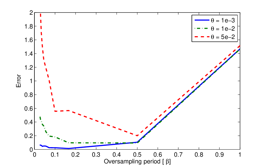
The error depends on the choice of generator and the oversampling period , as seen in Figure 6. The relationship between the kernels and the optimal oversampling period is still not evident.
6. Acknowledgements
The second and fourth authors were supported by NINDS (Grant Number: NS053561). The third author was partially supported by the following grants: PICT06-00177, CONICET PIP 112-200801-00398 and UBACyT X149. The third and fourth authors’ visit to the Numerical Harmonic Analysis Group (NuHAG) of the University of Vienna was funded by the European Marie Curie Excellence Grant EUCETIFA FP6-517154.
References
- [1] A. Aldroubi. Non-uniform weighted average sampling and reconstruction in shift-invariant and wavelet spaces. Appl. Comput. Harmon. Anal., 13(2):151–161, 2002.
- [2] A. Aldroubi and K. Gröchenig. Nonuniform sampling and reconstruction in shift-invariant spaces. SIAM Rev., 43(4):585–620, 2001.
- [3] A. Alvarado, J. Principe, and J. Harris. Stimulus reconstruction from the biphasic integrate-and-fire sampler. In Neural Engineering, 2009. NER ’09. 4th International IEEE/EMBS Conference on, pages 415–418, April 29 2009-May 2 2009.
- [4] D. Chen, Y. Li, D. Xu, J. Harris, and J. Principe. Asynchronous biphasic pulse signal coding and its cmos realization. Circuits and Systems, 2006. ISCAS 2006. Proceedings. 2006 IEEE International Symposium on, pages 4 pp.–2296, 0-0 2006.
- [5] H. G. Feichtinger. Banach convolution algebras of Wiener type. In B. Sz. Nagy and J. Szabados, editors, Proc. Conf. on Functions, Series, Operators, Budapest 1980, volume 35 of Colloq. Math. Soc. Janos Bolyai, pages 509–524, Amsterdam, 1983. North-Holland.
- [6] H. G. Feichtinger. Wiener amalgams over Euclidean spaces and some of their applications. In K. Jarosz, editor, Function Spaces, Proc Conf, Edwardsville/IL (USA) 1990, volume 136 of Lect. Notes Pure Appl. Math., pages 123–137, New York, 1992. Marcel Dekker.
- [7] H. G. Feichtinger and K. Gröchenig. Theory and practice of irregular sampling. In J. Benedetto and M. Frazier, editors, Wavelets: Mathematics and Applications, Studies in Advanced Mathematics, pages 305–363, Boca Raton, FL, 1994. CRC Press.
- [8] W. Gerstner and W. Kistler. Spiking neuron models. Cambridge University Press, 2002.
- [9] A. A. Lazar and E. A. Pnevmatikakis. Reconstruction of sensory stimuli encoded with integrate-and-fire neurons with random thresholds. EURASIP Journal on Advances in Signal Processing, 2009, July 2009.
- [10] A. A. Lazar, E. K. Simonyi, and L. T. Toth. A Toeplitz formulation of a real-time algorithm for time decoding machines. In Proceedings of the Conference on Telecommunication Systems, Modeling and Analysis, November 2005.
- [11] A. A. Lazar and L. T. Toth. Time encoding and perfect recovery of bandlimited signals. In IEEE International Conference on Acoustics, Speech and Signal Processing, volume 6, pages VI709–712, April 2003.
- [12] F. Rieke, D. Warland, de Ruyter, and W. Bialek. Spikes: Exploring the Neural Code. The MIT Press, 1997.
- [13] J. C. Sanchez, J. C. Principe, T. Nishida, R. Bashirullah, J. G. Harris, and J. A. B. Fortes. Technology and signal processing for brain-machine interfaces. Signal Processing Magazine, IEEE, 25(1):29–40, 2008.
- [14] H. Schwab. Reconstruction from Averages. PhD thesis, Dept. Mathematics, Univ. Vienna, 2003.
- [15] W. Sun and X. Zhou. Reconstruction of band-limited functions from local averages. Constr. Approx., 18(2):205–222, 2002.
- [16] D. Wei. Time based analog to digital converters. PhD thesis, University of Florida, 2005.