Hadron-hadron interaction from SU(2) lattice QCD
Abstract
We evaluate interhadron interactions in two-color lattice QCD from Bethe-Salpeter amplitudes on the Euclidean lattice. The simulations are performed in quenched SU(2) QCD with the plaquette gauge action at and the Wilson quark action. We concentrate on S-wave scattering states of two scalar diquarks. Evaluating different flavor combinations with various quark masses, we try to find out the ingredients in hadronic interactions. Between two scalar diquarks (, the lightest baryon in SU(2) system), we observe repulsion in short-range region, even though present quark masses are not very light. We define and evaluate the “quark-exchange part” in the interaction, which is induced by adding quark-exchange diagrams, or equivalently, by introducing Pauli blocking among some of quarks. The repulsive force in short-distance region arises only from the “quark-exchange part”, and disappears when quark-exchange diagrams are omitted. We find that the strength of repulsion grows in light quark-mass regime and its quark-mass dependence is similar to or slightly stronger than that of the color-magnetic interaction by one-gluon-exchange (OGE) processes. It is qualitatively consistent with the constituent-quark model picture that a color-magnetic interaction among quarks is the origin of repulsion. We also find a universal long-range attractive force, which enters in any flavor channels of two scalar diquarks and whose interaction range and strength are quark-mass independent. The weak quark-mass dependence of interaction ranges in each component implies that meson-exchange contributions are small and subdominant, and the other contributions, ex. flavor exchange processes, color-Coulomb or color-magnetic interactions, are considered to be predominant, in the quark-mass range we evaluated.
Keywords:
SU(2) lattice QCD, hadronic interaction, hadronic potentialpacs
12.38.Gc, 12.39.PnI Introduction
Hadron-hadron interactions play important roles in nuclear and hadron physics. Among them baryon-baryon interaction is one of the most important issues to be clarified in reliable manners: Baryons are the main building blocks of our world and their interactions are essential for the structures and dynamics of nuclei. After the successful proposal by Yukawa in 1935 [1], the long- and the intermediate-range interactions have been described by one-boson-exchange potentials (OBEP) [2, 3, 4]. The key players for the hadronic interactions in these regions are considered as mesonic modes. On the other hand, the short-range part of the interactions has not been well clarified so far. Especially, the origin of the large repulsive core in nucleon-nucleon (NN) channel [5], which accounts for the high-density nuclear phenomena, has been one of the longstanding problems in hadron physics [6, 7, 2, 8, 9, 10, 11, 12, 13, 14, 15]. The degrees of freedom of quarks and gluons would be essential in such short-distance region, and hence they should be clarified directly in terms of the fundamental theory, Quantum ChromoDynamics (QCD).
It is now common knowledge that all the hadronic systems are governed by QCD, and it is long after QCD was established as the fundamental theory. Nevertheless, QCD-based description of hadronic systems has not yet been successful due to the strong coupling nature of the low-energy QCD, whose dynamics is far from the perturbative regime and essentially nonperturbative. Among potentially workable strategies for nonperturbative analyses of QCD, lattice QCD is a unique reliable method for low-energy QCD. It can now reproduce empirical hadronic masses with a very good accuracy [16], and its outcome can be directly compared with experiments. There have been several attempts which aim at clarification of interhadron interactions by means of lattice QCD [17, 18, 19, 20, 21]. Recently, a nucleon-nucleon (NN) interaction was evaluated from NN Bethe-Salpeter (BS) amplitudes on the lattice [22], where the short-range repulsion and the attraction in the intermediate region were observed. While the information of scattering phase shifts are properly encoded in asymptotic BS amplitudes, “potentials” directly constructed from BS amplitudes have setup- (operator- or energy-) dependences. Nevertheless, they are considered useful to gain qualitative understanding of hadronic interactions.
In this article, we employ SU(2) lattice QCD, and investigate hadronic interactions aiming at clarifying the essential structure of them. First, the scalar diquark (, the lightest baryon in SU(2) system) is an isospin-zero scalar hadronic state in SU(2) QCD and some of possible one-meson-exchange channels in diquark interactions are restricted, and hence analyses could be simpler. Diquarks in SU(2) QCD have a direct connection to mesons, and two-diquark correlators are identical with two-meson correlators if we neglect possible quark-disconnected diagrams. Second, while SU(2) and SU(3) QCDs have different natures in some situations [23, 24], they often show similar aspects [25], and hence SU(2) QCD can be a testbed for understanding hadron interactions. On the lattice, it is possible to switch on/off Pauli-blocking effects among quarks controlling flavor contents or equivalently quark-exchange diagrams, which enables us to classify hadronic interactions in terms of their origins.
II Formulation
We follow the strategy proposed by CP-PACS group [26], where asymptotic Bethe-Salpeter wavefunctions on the Euclidean lattice are adopted to evaluate pion scattering length. This method has been further employed for various hadron-hadron channels [27, 28].
We measure a two-diquark correlator at Euclidean-time , which is defined as
| (1) | |||
| (2) |
Here, represents the relative coordinate of two scattering hadrons, and and are interpolating fields for diquark states whose flavors are and . is defined with two quark fields,
| (3) |
with being the anti-symmetric tensor. Spinor indices of the two quark fields in are contracted with . Possible ’s are , , and , which respectively correspond to pseudo-scalar, scalar, axialvector, and vector diquarks. We employ wall-type operators for sources, while we use point-type operators for sinks. After Euclidean-time evolution, a system is finally dominated by the ground-state, and loses -dependence besides an overall constant and an exponential damping factor. The BS wavefunction is then obtained as .
With such , we can define an -dependent function assuming a nonrelativistic Schrödinger-type equation,
| (4) |
Thus extracted scattering-energy dependent function is an equivalent potential which reproduces the scattering phase shift at the target energy. Though the information of phase shift is properly encoded in such equivalent potentials , they could be energy- and operator-dependent. In this sense, equivalent potentials contain no more definite information than phase shifts in asymptotic region. Nevertheless, equivalent potentials are expected to be useful to gain understanding of hadronic interactions, at least qualitatively. We extract equivalent potentials, which we simply call as “potential” in this paper, and evaluate hadronic interactions in SU(2) QCD.
We concentrate on S-wave scattering states of two scalar diquarks (), and we project wavefunctions onto -wavefunction , which has overlap with states, by summing over in terms of corresponding discrete rotations. We here neglect the contributions from scattering states, since such contributions can be dropped by taking large Euclidean time .
All the simulations are performed in SU(2) quenched QCD with the standard plaquette gauge action and the Wilson quark action. The lattice size is at , whose lattice spacing is about 0.1 fm if we assume is 440 MeV [29, 30]. We employ four different Hopping parameters = 0.1350, 0.1400, 0.1450, 0.1500 for quarks. Diquarks at these ’s would be well described by conventional quark models, and Nambu-Goldstone-boson nature does not emerge. (See Secs. III.1 and V.2.)
III Lattice QCD results
III.1 Hadron masses
We show the lowest-state diquark masses in each channel in Table 1. The masses are extracted in a standard manner. We fit hadronic correlators by a single-exponential function, . We do not need “quark-annihilation” diagrams in the computation of diquark correlators. The scalar, vector, pseudoscalar, axialvector () channels are investigated.
Fig. 1 shows the mass difference between scalar and axialvector diquarks. The dashed line denotes the fit function, , where is the half of the axialvector-diquark (vector-meson) mass. The mass splitting is clearly proportional to , which supports the color-magnetic interaction as the origin of the mass splitting and indicates the validity of nonrelativistic-quark-model description of scalar and axialvector diquarks, at least in the quark-mass range we consider. In the picture of constituent quark model, if spatial wave functions of constituent quarks in diquarks are affected by quark-mass variation, the dependence of the mass splitting can be modified from the scaling, which originates from the factor of the strength of the color-magnetic interaction. The almost perfect -behavior of the mass splitting then implies that the spatial wave functions in these two diquarks are similar and less dependent on quark mass.

| Scalar | Axialvector | Pseudoscalar | Vector | ||
| 0.1350 | 1.044(2) | 1.056(2) | 1.285( 2) | 1.286( 3) | 0.012(2) |
| 0.1400 | 0.836(2) | 0.855(2) | 1.102( 2) | 1.102( 4) | 0.019(2) |
| 0.1450 | 0.618(2) | 0.651(2) | 0.919( 4) | 0.918( 5) | 0.033(2) |
| 0.1500 | 0.377(3) | 0.447(2) | 0.757( 7) | 0.728( 4) | 0.070(3) |
| 0.1150 | 1.020(2) | 1.026(2) | 1.397( 9) | 1.352( 8) | 0.006(2) |
| 0.1250 | 0.494(2) | 0.504(1) | 1.053(25) | 0.889(19) | 0.010(2) |
III.2 Wavefunctions
We hereby consider two-scalar-diquark wavefunctions with two different flavor combinations. One combination is , where only two independent flavors exist in four quarks. The other is , where all the quarks have different flavors. We adopt the same hopping parameters (quark masses) for all the quarks in both cases, and therefore all the scalar diquarks degenerate in mass. We note that the diagrams for the channel consist of direct and quark-exchange diagrams, and the direct diagrams in the channel are identical with those needed for the channel. “Quark-exchange diagrams” in quark-propagator contraction are included only in the case. The existence of quark-exchange diagrams would be essential for the short-range interactions, since any Pauli-blocking effects among quarks are not included without exchange diagrams. We expect that the origin of short-range hadronic interactions can be accessed by comparing these two flavor combinations.


We refer to the determination of wavefunctions . Law wavefunctions depend on the source-sink separation due to possible excited-state contaminations. We then have to take enough large to ensure the absence of such contaminations. For this aim, we extract -dependent wavefunctions and determine -window where excited-state contaminations are negligible. Fig. 2 shows -dependent wavefunctions at =0.1500 as functions of source-sink separation . The upper and lower panels correspond to and cases, respectively. They show plateaus at , and we then extract “wavefunctions” by fitting the data as at . For further confirmation, we look at -dependent potentials extracted directly from . In Fig. 3, -dependent potentials (=1,2,4) at =0.1500 are shown. One can find that they consistently show plateaus at .

In Fig. 4, as an example, we show the wavefunctions as functions of the relative distance for four different ’s.The flavor combinations are all .
III.3 Potentials : case
We next proceed with the potentials extracted from the wavefunctions. Fig. 5 shows the reconstructed potentials plotted as functions of , where the flavor combination is set to . In this case, we include no quark-exchange diagram and hence no Pauli-blocking effect among quarks is activated.
At a glance, one can find that the interaction in this channel is always attractive, and that the strength of this attraction depends on quark masses. The -dependence is monotonous at all the ’s. In the large region (), the potential has smaller dependence, while it has strong dependence in the short-distance region (). The potential rapidly reduces with decreasing (increasing ), and finally the potentials at =0.1350 and 0.1400 coincide with each other. The potential exhibits saturation at heavy quark-mass region, which implies a long-range quark-mass independent attraction. Although quark masses are also responsible for hadron size itself and would indirectly affect interhadron potentials, these effects seem small in the present quark-mass range.

III.4 Potentials : case
The interhadron potentials with the flavor combination can be seen in Fig. 6. The difference from the previous case is that quark-exchange diagrams are now included, which gives rise to Pauli-blocking effect among quarks.
We readily find that strong repulsions in the short-distance region appear in this case. Compared with the case, the quark-mass dependence is not monotonous: They are smooth functions of at large ’s, while the potential at =0.1350 has a pocket at the intermediate distance. As the quark mass decreases, the short-range repulsive part rapidly grows up and the intermediate attractive pocket disappears. Such qualitative change in shape suggests that the potentials in case consist of two or more parts; attractive part and (probably) repulsive part whose strengths and quark-mass dependences are different from each other.

III.5 Potentials : Quark-exchange part
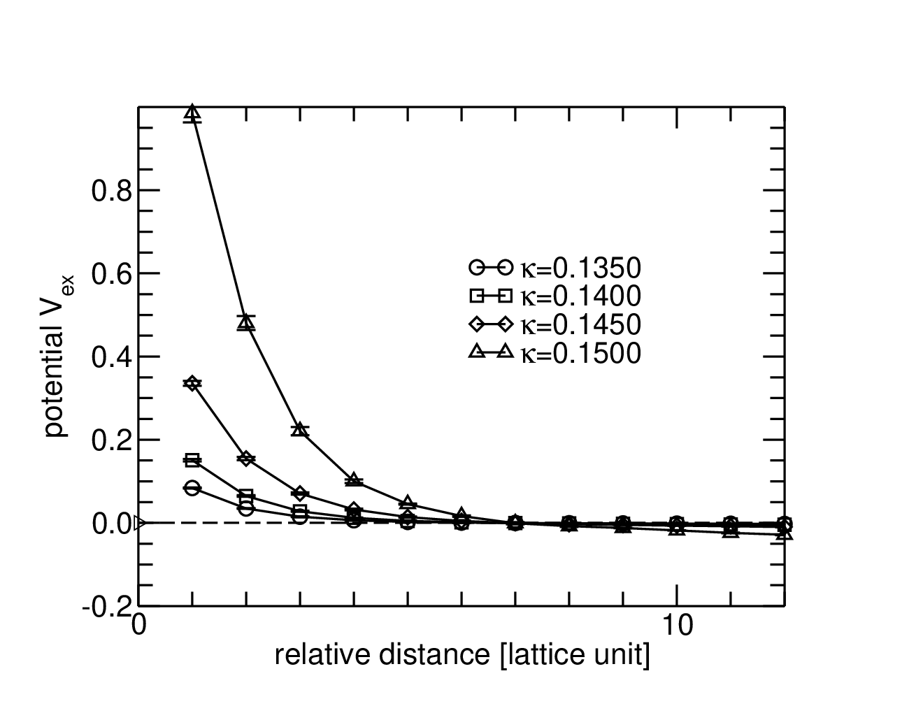
In the following, we define a “quark-exchange part” in as
| (5) |
which is nothing but the difference between and . Taking into account that quark-exchange diagrams are included only in the case of and that the diagrams needed for are identical with the direct diagrams in , it gives a measure of “quark-exchange effect” or Pauli-blocking effect among quarks in the potential . In practice, it is equivalent to assuming
| (6) | |||
| (7) |
for and , with a “direct part” measured only with direct diagrams and a “quark-exchange part” induced by adding exchange diagrams or equivalently by introducing Pauli blocking among quarks. Such decomposition of a diquark-diquark potential is conceptually similar to the usual decomposition procedure in RGM (Resonating Group Method) calculations in quark cluster models [31, 11, 12]. In case multiply repeated quark-exchange processes can be neglected, like the Born approximation, these two components, and , result in so-called direct and exchange potentials, respectively. Thus extracted potential shows a monotonous behavior as is seen in Fig. 7, and therefore the decomposition seems beneficial for our purpose to clarify strengths or ranges of potentials. At the same time, one finds that the short-range repulsion arises only from . Pauli-blocking effect among quarks is essential for the short-range repulsion.
IV Discussions
Now that we have extracted the ingredients of each potential. Namely, and are expressed as
| (8) | |||
| (9) |
and can be regarded as the origins of attractive and repulsive interactions, respectively.
The key property of the -dependent potentials is twofold; interaction ranges and strengths. Their -dependences are also helpful to clarify the origins of the potentials. In phenomenological models, hadronic interactions are usually incorporated as one-boson-exchange-potentials (OBEP), which are Yukawa-type and whose interaction ranges are directly connected to (exchanged) meson masses. Then, such OBE potentials should be sensitive to meson masses, i.e. quark masses. On the other hand, the short-range repulsive core is often considered to arise from a color-magnetic interaction induced by one-gluon-exchanges (OGE), whose strength is proportional to the inverse square of (probably constituent) quark masses, . Such -dependent interactions could be accessed by monitoring the strengths of the potentials.
In this section, we evaluate strengths and ranges of these decomposed potentials, and , together with their -dependences. Since we do not have priori function forms, especially for the short-range repulsive part, we try the following five trial functions, , which have two parameters, strength and range .
| (10) |
| (11) |
| (12) |
| (13) |
| (14) |
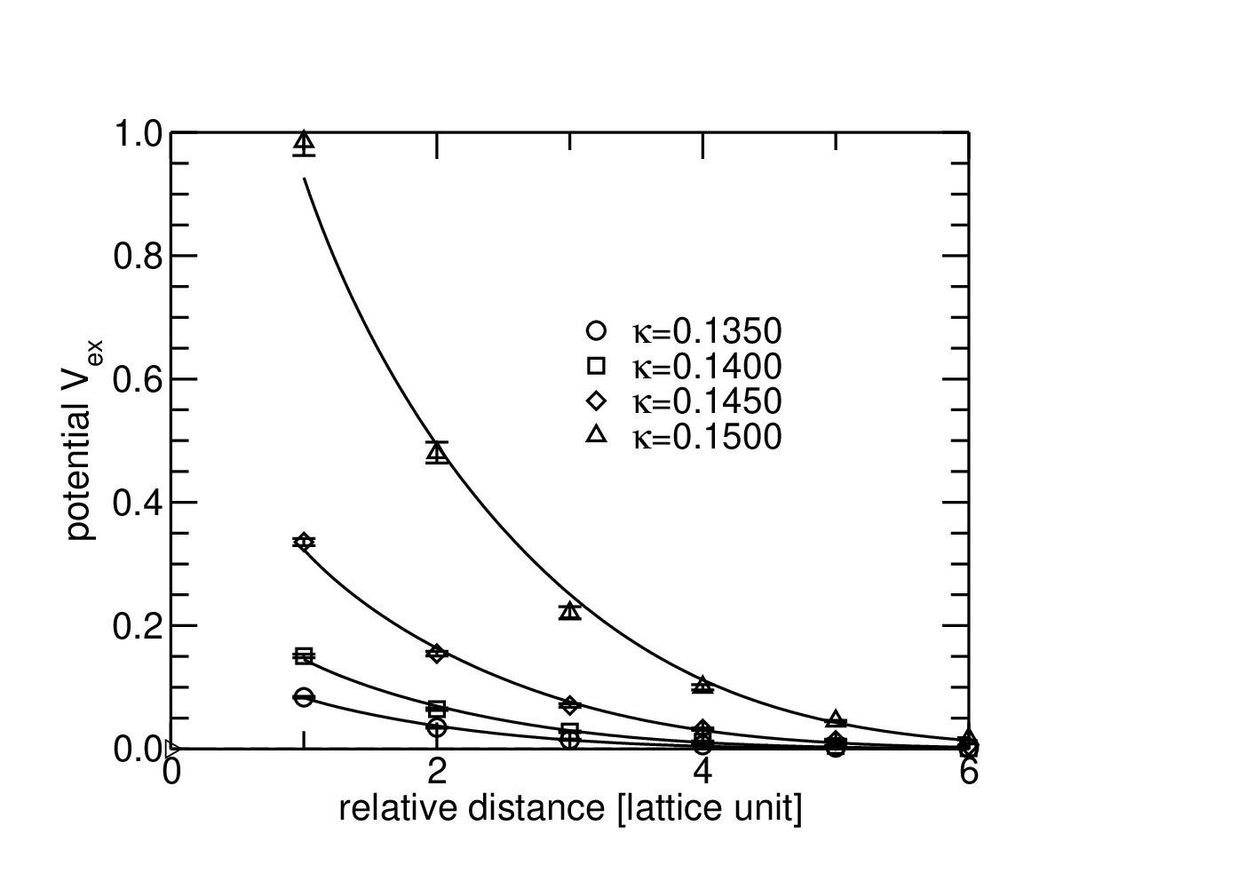
The fit results can be all found in Table. 2, in which , strengths and ranges for and at each are listed. None of five functions produces for all the data, which would be due to the lack of knowledge about detailed function forms, some systematic errors in the lattice data, and possible multi-range components, which will be discussed later. We adopt as the fit function, since it yields relatively smaller for any combination of potential type and quark mass. For reference, we plot (best-fit) ’s and the lattice data in Fig. 8. The lattice data are rather well mimicked by the function.

| 0.1350 | 0.1400 | 0.1450 | 0.1500 | |
| 1.462 | 1.719 | 12.24 | 3.163 | |
| 54.50 | 6.970 | 0.381 | 9.037 | |
| 8.938 | 1.094 | 3.516 | 2.206 | |
| 33.78 | 3.725 | 0.094 | 11.33 | |
| 85.32 | 15.00 | 3.818 | 30.43 | |
| 0.046(001) | 0.050(002) | 0.081(009) | 0.345(007) | |
| 0.015(004) | 0.017(003) | 0.032(001) | 0.144(010) | |
| 0.154(010) | 0.171(006) | 0.294(019) | 1.134(024) | |
| 0.073(013) | 0.083(008) | 0.162(002) | 0.655(050) | |
| 0.011(008) | 0.015(007) | 0.046(007) | 0.206(052) | |
| 4.24(006) | 4.33(011) | 3.87(024) | 2.58(005) | |
| 7.06(150) | 6.77(076) | 5.36(010) | 3.61(020) | |
| 1.93(008) | 1.91(005) | 1.62(007) | 1.16(002) | |
| 3.27(041) | 3.11(021) | 2.42(002) | 1.72(011) | |
| 10.3(060) | 8.12(277) | 4.63(050) | 3.20(058) | |
| 0.1350 | 0.1400 | 0.1450 | 0.1500 | |
| 3.869 | 5.317 | 6.064 | 7.543 | |
| 0.546 | 1.144 | 3.713 | 4.562 | |
| 0.095 | 0.481 | 0.737 | 2.202 | |
| 1.871 | 4.896 | 8.627 | 13.19 | |
| 8.460 | 16.28 | 27.94 | 33.92 | |
| 0.060(003) | 0.099(006) | 0.209(012) | 0.565(036) | |
| 0.025(001) | 0.046(002) | 0.094(006) | 0.277(016) | |
| 0.201(002) | 0.354(008) | 0.744(017) | 2.188(085) | |
| 0.119(007) | 0.223(020) | 0.453(046) | 1.424(163) | |
| 0.040(010) | 0.089(023) | 0.168(050) | 0.606(152) | |
| 2.58(010) | 2.78(010) | 2.99(010) | 3.25(007) | |
| 3.58(008) | 3.63(009) | 3.95(015) | 3.97(009) | |
| 1.14(001) | 1.17(002) | 1.27(002) | 1.29(002) | |
| 1.67(008) | 1.64(009) | 1.80(012) | 1.72(008) | |
| 2.98(048) | 2.61(041) | 2.98(055) | 2.60(030) | |
| 0.1350 | 0.1400 | 0.1450 | 0.1500 | |
| N/A | N/A | 1.338 | 0.246 | |
| N/A | N/A | 0.186(024) | 1.041(046) | |
| N/A | N/A | 1.05(009) | 1.01(004) |
IV.1 strengths and ranges :
In Table 2 and Fig. 9, we show the fitted parameters, strength and range of the attractive part , as functions of half of axialvector-diquark mass. (Shown as “DIR” in Fig. 9.) Interestingly enough, both of the strength and the range of exhibit flattening in the heavy quark-mass region, which indicates that contains a universal attractive potential . “Universal” here means that neither the strength nor the range of depends on quark mass and that always appears in any flavor channels. In fact, an attractive “dip” at the intermediate range in seems to originate from this universal attractive potential . The combination of -dependent short-range repulsive force and -independent long-range attractive force provides a dip at the intermediate range.
In much heavier quark-mass region, the properties of quark wavefunctions would undergo gradual change, and could be quark-mass dependent. However, in the quark-mass range we consider here, can be treated as a fixed function.
Then, the next question is what the reminder is. We define the quark-mass dependent part as
| (15) |
We also fit with , and the fitted parameters are shown in Table 2 and Fig. 9. Here, we simply adopt at as the universal part , since we observe almost no quark-mass dependence already at this . The strength and the range of are shown as “ATT(D)”. The extracted range is no longer dependent on quark mass. That is, is approximately described by two independent parts;
| (16) | |||||
| (17) |
First part represents a -independent weak long-range force, and the second one does a short-range repulsive interaction that has an -dependent strength and an -insensitive interaction range. Possible origins of the universal attraction would be transition processes to other two hadronic (intermediate) states, which is schematically illustrated in the left panel of Fig. 10, or -independent gluonic interactions. As the candidates for -independent gluonic interactions, one can consider color-Coulomb interaction, medium-range attractions due to flavor exchange processes, and so on, since no quark-mass dependence is observed. As is found also in our analyses, such a weak universal attractive force is readily masked by the strong repulsive force in the potential for lighter quark-mass.
IV.2 strengths and ranges :


In Table 2 and Fig. 9, we show the fitted parameters, strength and range of the quark-exchange part , as functions of half of axialvector-diquark mass. (Shown as “EX” in Fig. 9.) Let us first have a look at the range parameter , which are shown as “EX” in Fig. 9. One can find that the range in is almost quark-mass independent. It is interesting since the repulsive cores are sometimes described by e.g. omega-meson exchanges in phenomenological models. The constituent quark-mass (half of AV-diquark mass) variation from 0.53 to 0.22 gives rise to only 10% change in the range , which is much smaller than expected from the meson-mass change. Moreover, at two largest ’s (two lightest quark masses), the range remains unchanged. can be predominantly expressed as
| (18) |
The quark-mass dependence (approximately) appears only in the strength . From these observations, we conjecture that the short-range repulsion is not generated by meson poles as OBEP, but by some other origins.
One most possible mechanism for the short-range repulsion is a color-magnetic (CM) interaction among quarks as suggested by constituent-quark models. A CM interaction accompanied by Pauli blocking among quarks raises the energy of (closely located) two hadrons, which results in strong repulsions. In the first-order perturbation, the contributions from the CM interaction are proportional to its strength, whose -dependence is given by .
The strengths extracted by fits are also shown in Table 2 and Fig. 9. increases in the light-quark-mass region and it is qualitatively consistent with the CM interaction as the origin of repulsion. In the upper panel in Fig. 9, two fit functions, and are respectively plotted as a long-dashed and a dashed line. The strength is well reproduced by rather than , which implies that the quark-mass dependence of repulsion seems stronger than that of the strength of the CM interaction itself. However, considering that the Pauli blocking among quarks is essential for the repulsion and that the interaction range of the repulsive force has a very weak quark-mass dependence, the present results are consistent with the quark-model interpretation that short-range repulsion between hadrons arises from CM interaction among quarks.
V Some additional trials
V.1 Boundary condition dependences
In the previous section, we claimed that one possible contribution for the universal attraction would be transition processes to other two hadronic (intermediate) states, which is schematically illustrated in the left panel of Fig. 10.

In case that two hadrons are closely located, it may not be meaningful to identify their flavors, because in such short-distance regions, two hadrons are largely overlapping with each other and they may differ from two isolated hadrons [31, 32].
In order to get sure that we have no finite-volume artifact for the universal attraction, we repeat the same analyses with antiperiodic spatial boundary conditions [33, 34]. The flavors are again , and anti-periodic boundary conditions are imposed for -flavor quark fields. In this case, - two-diquark state is never affected, since - and -diquarks obey a periodic boundary condition. If there exists finite-volume artifact in intermediate transition states, e.g. - hadronic state, the results would be modified in this new analysis. We eventually observed no modification in all the cases, and no serious finite volume effect is confirmed.
V.2 Removal of high-momentum gluons
Hadronic interactions may be classified into two categories. One is highly nonperturbative phenomena, such as meson interactions, and the other is perturbative contributions represented as CM interactions among quarks. In one sense, these phenomena differs in energy scale they belong to. Recently, a method that restricts energy scale of gluons via the Fourier transformation was proposed and tested [35, 36]. The authors reported that removal of high-energy contributions results in vanishing short-range Coulomb interaction in heavy-quark potentials, keeping the linear confinement part still unchanged. Taking into account that the Coulomb potential in short-distance region comes from OGE processes, removal of high-energy gluons is expected to cut such OGE processes. Though it should be clarified whether such removal also cuts other OGE interactions, e.g. color-magnetic part, this analyses might give us a hint to short-range hadronic interactions. Especially, the origin of short-range repulsive core coming from the color-magnetic OGE interaction would be accessed to some extent in this manner.
We perform 3-dim Fourier transformation [37] for link variables in the Landau gauge and extract in momentum space:
| (19) |
We leave the low-momentum contribution,
| (20) |
and reconstruct new SU(2) link variables in the coordinate space, , so that the distance,
| (21) |
is minimized. Here,
| (22) |
is a truncated link variable reconverted into the coordinate representation, which no longer belongs to SU(2). The infrared cut is set to in lattice unit.

We show the interquark potential in Fig. 11. The upper data in Fig. 11 shown as circles denote the lattice QCD data obtained in full SU(2) calculation, and the lower data shown as squares denote those obtained without high-momentum gluons. The original -potential data is fitted with the Cornell type potential as, . On the other hand, a fit of using the Cornell type potential seems not applicable due to the oscillation behavior in the short-range regions. We simply draw a dotted line, , in the figure. One can find that the short-distance Coulomb interaction disappears and the linear confinement part remains almost unchanged. At the same time, the constant part in the potential, which represents the self energy of a static fundamental charge under the lattice regularization, also disappears in this treatment.
An interesting observation can be found in the masses of scalar and axialvector diquarks. We adopt two hopping parameters = 0.1150 and 0.1250. We note here that we have adjusted ’s to cover approximately the same quark-mass region so that the AV-diquark masses before and after high-momentum-gluon cut are similar. In Table. 1, we list the masses of scalar(S) and axialvector(AV) diquarks. The masses measured with low-momentum link variables almost show no mass splitting, which implies that the color-magnetic interaction that gives rise to S-AV mass splitting is now largely suppressed. The fact that S- and AV-diquark masses degenerate in this manner again implies the validity of nonrelativistic-quark-model description of the diquarks. The NG-boson nature in S-diquark hardly appears in the present quark-mass region.


We show the interhadron potentials measured with the low-momentum link variables in Figs. 12, 13, and 14. Naive expectation is that potentials originating from short-range OGE processes are suppressed, while those from other origins remain unchanged. Actually, all the potentials get smaller after the high-momentum gluons are removed, which can be seen in Figs. 12, 13, and 14. The -dependence of potentials are also much milder now, and the divergent behavior around the origin disappears. The reason why all are now decreased could be that many of the hadronic processes, e.g. flavor exchanges, meson exchanges, and so on, need color recombinations in hadrons. If such recombinations are prohibited, some of hadronic processes depending on them will be also suppressed.

To clarify the origin of repulsion in a clearer way, we plot the values of at =1 and 2 as functions of S-AV mass splitting in Fig. 15. The open symbols are the original data taken from fully calculated potential , and the filled symbols denote the values of obtained without high-momentum gluons. Open and filled symbols are compared at the same . While the open symbols show behavior, the filled symbols deviate from the expected curve and always lie above it, which indicates that the repulsive interaction does not always decrease like the S-AV mass splitting, and that some extra enhancement remains even after the high-momentum-gluon cut. We then expect that the repulsive force still contains small contributions other than CM interaction among quarks.
Restricting gluon’s energy scale surely changes potentials and may be useful to clarify detailed structures. However, there seem to remain several issues to be clarified before quantitative conclusions are reached.
V.3 Different choice in operators
Concern about possible operator dependences of potentials from BS amplitudes has been often raised [38]. BS amplitudes themselves are operator-dependent quantities, and inevitably equivalent potentials extracted from them are. Though the strengths and the ranges of the potentials would be operator dependent, some essential features in hadronic interactions will be clarified by investigating operator dependences. Among possible hadronic operators, we hereby consider spatially extended smeared operators, because hadron-size effect is considered to be one of the most important features: Hadronic states have finite sizes, and hence finite-size (smeared) hadronic operators would be more adequate to describe hadrons. We note that the reduction formula needed to relate BS amplitudes to scattering observables has been proved only for point-type operators [39, 40, 41, 42]. In this subsection, we repeat our analyses employing smeared operators for sinks in order to derive essentials in hadronic interactions.
First, we mention smearing methods. Usually, quark operators are individually smeared, and hadronic operators are constructed from them. In the case of gauge-invariant Gaussian smearing, each quark operator is smeared with a gauge-covariant lattice derivative operator
| (23) |
as
| (24) |
Parameters and are chosen so that quark fields are distributed around with a radius . We hereby consider diquark states which consist of two quarks with identical masses. A smeared hadronic (diquark) operator whose center position is is then defined with and as . However, in reality, does not describe a hadronic state located at , but it contains unwanted contributions because a “position” of a hadron, , does not always coincide with . For example, has nonzero entry at , which is nothing but a point-type hadronic operator located at . While such contributions are not harmful in hadron-mass measurement because hadronic states are projected onto a momentum eigenstate summing up hadronic correlators, it causes serious difference in the measurement of BS amplitudes. should be zero when . In order to satisfy the condition , we improve smearing function with the following prescription.
With new link variables, , and a phase , we define
| (25) | |||||
| (26) | |||||
| (27) |
Smeared quark operators are similarly defined as
| (28) |
Here, can be chosen freely. As a result, are different from in overall phases;
| (29) |
For simplicity, we hereby consider a hadronic operator located at the origin, . Then, a hadronic (diquark) operator is now
| (30) | |||||
| (31) | |||||
| (32) |
Taking ,
| (33) | |||||
| (34) |
If we average as over so that , the “position” of a hadronic operator can be unambiguously defined. ( is always satisfied.) The simplest choice is averaging it over a random set . This scheme is a generalization of projection processes, and could be employed for other purposes.
We note here that nothing other is changed in this process. A hadronic operator is now “projected” onto ()-state so that unwanted contributions are absent. In actual calculations, are averaged over the set . When is smaller than the lattice spatial extent, the delta function is not fully reproduced and the projection is incomplete. To eliminate such (small) contaminations, we further introduce overall random phases.
Next, we measure hadron “sizes” monitoring overlap coefficients. The sink operators relevant to BS amplitudes are now smeared in a gauge invariant way. The root-mean-square radius of the smeared operators are determined so that the smeared operators have maximal overlaps with the ground states (scalar diquarks).

In Fig. 16, we plot the squared overlaps, . Here, denotes the overlap of a diquark operator and -th state, which is defined as
| (35) |
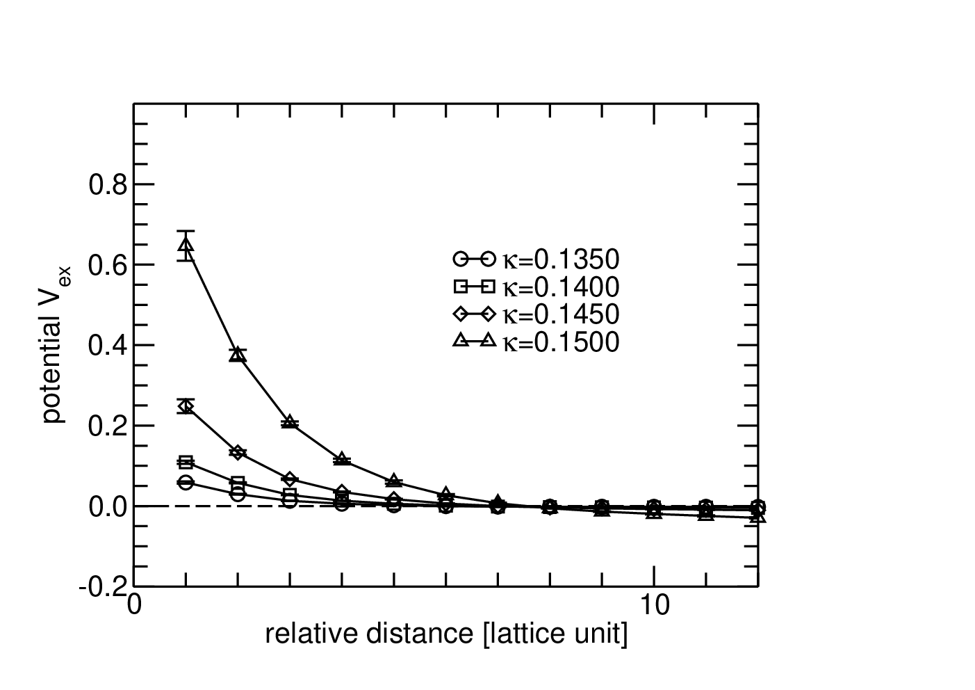
While the squared overlaps are slightly dependent on quark masses, they are saturated at . We then set for all the ’s. In Figs. 17-19, we show ,, and obtained with “properly projected” smeared operators.
obtained with smeared operators are qualitatively similar to those with point operators. It is always attractive and gets stronger at smaller quark-mass region. Especially, the saturation at heavy region can be again seen in Fig. 17. The interaction range of the universal attractive potential is now reduced by about 20%, and the strength is stronger, compared with the universal attraction observed in the point-operator case. On the other hand, repulsive cores in at short-distance region are generally weaker in this case, which is displayed in Fig. 18. Apparent repulsive cores disappear at small ’s, whereas cores still persist and are observed at larger ’s. seems more sensitive to operator choice than . Interestingly, the difference still hold similar properties to that in point-operator case. It grows as decreases and is always repulsive, which confirms that the Pauli-blocking effect is responsible for repulsion also in this case. The interaction range of remains almost unchanged as compared to that extracted with point operators.
Quantitative evaluation of interhadron potentials seems difficult at present, because of its operator dependences. However, several basic properties remain qualitatively unchanged with/without operator smearing: (1) The existence of universal attraction between two hadrons. (2) The difference still shows repulsive contribution at any ’s. (3) The quark-mass dependences of the interaction ranges of direct () and exchange () parts of potentials are much weaker than expected from meson exchanges. (4) The quark-mass dependence of the strength of is consistent with or stronger than .




All the parameters are obtained by fitting potentials measured with “projected” smeared diquark operators .
VI Summary and Outlooks
We have evaluated inter-hadron interactions in two-color lattice QCD based on the -dependent function . The function , which has been expressed as “potential” throughout this paper, has been extracted from the Bethe-Salpeter wave functions on the lattice assuming a nonrelativistic Schrödinger equation. The simulations have been performed in quenched two-color QCD with the plaquette gauge action at and the Wilson quark action. Evaluating different flavor combinations as well as several quark masses, we have extracted and investigated each ingredient in hadronic interactions. We have considered two-diquark scatterings, whose flavors are and . When all the quarks have different flavors, , the interhadron potential is quark-mass dependent and always attractive,
| (36) |
On the other hand, in channel, where exchange diagrams, i.e. Pauli-blocking effect among quarks, are included, shows repulsion in short-distance region, and this repulsion arises only from the exchange diagrams. We have defined the “quark-exchange part” in the potential, which is induced by adding quark-exchange diagrams, or equivalently, by introducing Pauli blocking among some of quarks. Namely, when some of the quarks have identical flavors, , the quark-exchange part is defined as , which means the interhadron potential is written as
| (37) |
It indicates that the short-range repulsive core in arises only from the “quark-exchange part” . Pauli blocking among quarks seems essentially needed to generate repulsive force between two hadrons.
We have found that these - and -dependent contributions can be further decomposed into simpler parts;
| (38) | |||||
| (39) | |||||
| (40) |
Here, ’s are quark-mass independent functions of . Interestingly, can be further decomposed into and , a universal attractive part and an -dependent attractive part.
One prominent observation is that all the -functions , , and are quark-mass independent, which implies that the quark-mass dependences of and do not appear in interaction ranges but only in the overall strengths. Though we first adopted the specific function for potential-form analyses, we finally found that simple rescaling of the potential (the lattice data themselves) well explains all the quark-mass dependences. That is, we eventually encounter no scheme dependence in these descriptions. These observations apparently do not go together with the meson-exchange picture among hadrons, since -dependences of interaction ranges seem very small. At least in the present quark-mass range, mesonic contributions seem small and subdominant, and hence we observed interactions of the other origins.
For the repulsive part, we have found that the strength grows as , which is similar to but slightly stronger than the color-magnetic interaction itself by one-gluon-exchange (OGE) processes. Considering that the Pauli blocking among quarks is essential for the repulsion and the interaction range of the repulsive force has a very weak quark-mass dependence, it is likely to originate from a color-magnetic interaction among quarks.
Actually, the function is energy and operator dependent. In order to clarify operator dependence, we have constructed “projected” smeared operators and compared the results with and without operator smearing. As a result, we observed quantitative changes in potential shapes. Quantitative evaluation of interhadron potentials seems difficult at present, because of its operator dependences. On the other hand, several basic properties remain qualitatively unchanged with/without operator smearing: (1) The existence of universal attraction between two hadrons. (2) The difference still shows repulsive contribution at any ’s. (3) The quark-mass dependences of the interaction ranges of direct and exchange parts of potentials (,) are much weaker than expected from meson exchanges. (4) The quark-mass dependence of the strength of is consistent with or stronger than . To determine the precise forms of interhadron potentials, it would be necessary to perform more sophisticated analyses taking into account energy dependence in a less operator-dependent way.
Since quark-mass dependence in interaction ranges does not appear, the origin of the interactions we observed so far would be all gluonic interactions and/or flavor-exchange processes, e.g. color-magnetic or color-Coulomb interactions, and so on, rather than mesonic contributions. As was found in our analyses, attractive forces are readily masked by the strong repulsive force appearing in the potential in the light quark-mass region. If the universal attraction in hadronic interaction appears also in SU(3) QCD, they might be observed in a channel with no or less quark-exchange contribution between hadrons, such as scattering state. In the lighter quark-mass region, meson-exchange contributions could largely emerge and be predominant, which is left for further studies.
Acknowledgements.
All the numerical calculations were performed on NEC SX-8R at CMC, Osaka university, on SX-8 at YITP, Kyoto University. The authors thank Dr. K. Yazaki for discussions. This work was supported in part by the Yukawa International Program for Quark-Hadron Sciences (YIPQS), and the Grant-in-Aid for the Global COE Program “The Next Generation of Physics, Spun from Universality and Emergence” from MEXT of Japan, and by KAKENHI (20028006, 21740181).References
- [1] H. Yukawa, Proc. Phys. Math. Soc. Jap. 17, 48 (1935).
- [2] Prog. Theor. Phys. Suppl. 39 (1967).
- [3] Rev. Mod. Phys. 39, p495 (1967).
- [4] R. Machleidt, K. Holinde and C. Elster, Phys. Rept. 149, 1 (1987).
- [5] R. Jastrow, Phys. Rev. 81, 165 (1951).
- [6] S. Otsuki, M. Yasuno and R. Tamagaki, Prog. Theor. Phys. Suppl. 1965, 578 (1965).
- [7] V. G. Neudachin, Yu. F. Smirnov and R. Tamagaki, Prog. Theor. Phys. 58, 1072 (1977).
- [8] D. A. Liberman, Phys. Rev. D 16, 1542 (1977).
- [9] M. Harvey, Nucl. Phys. A 352, 326 (1981).
- [10] M. Oka and K. Yazaki, Phys. Lett. B 90, 41 (1980).
- [11] M. Oka and K. Yazaki, Prog. Theor. Phys. 66, 556 (1981).
- [12] M. Oka and K. Yazaki, Prog. Theor. Phys. 66,572 (1981).
- [13] A. Faessler, F. Fernandez, G. Lubeck and K. Shimizu, Phys. Lett. B 112, 201 (1982).
- [14] M. Oka and K. Yazaki, in Quarks and nuclei, ed. W. Weise (World Scientific, Singapore, 1984), p. 489 and references theirein .
- [15] M. Oka, K. Shimizu and K. Yazaki, Prog. Theor. Phys. Suppl. 137, 1 (2000).
- [16] S. Aoki et al. [PACS-CS Collaboration], Phys. Rev. D 79, 034503 (2009) [arXiv:0807.1661 [hep-lat]].
- [17] A. Mihaly, H. R. Fiebig, H. Markum and K. Rabitsch, Phys. Rev. D 55, 3077 (1997).
- [18] C. Stewart and R. Koniuk, Phys. Rev. D 57, 5581 (1998) [arXiv:hep-lat/9803003].
- [19] C. Michael and P. Pennanen [UKQCD Collaboration], Phys. Rev. D 60, 054012 (1999) [arXiv:hep-lat/9901007].
- [20] T. T. Takahashi, T. Doi and H. Suganuma, AIP Conf. Proc. 842, 249 (2006) [arXiv:hep-lat/0601006].
- [21] T. Doi, T. T. Takahashi and H. Suganuma, AIP Conf. Proc. 842, 246 (2006) [arXiv:hep-lat/0601008].
- [22] N. Ishii, S. Aoki and T. Hatsuda, Phys. Rev. Lett. 99, 022001 (2007) [arXiv:nucl-th/0611096].
- [23] J. B. Kogut, M. A. Stephanov and D. Toublan, Phys. Lett. B 464, 183 (1999) [arXiv:hep-ph/9906346].
- [24] J. B. Kogut, D. K. Sinclair, S. J. Hands and S. E. Morrison, Phys. Rev. D 64, 094505 (2001) [arXiv:hep-lat/0105026].
- [25] G. S. Bali, K. Schilling and C. Schlichter, Phys. Rev. D 51, 5165 (1995) [arXiv:hep-lat/9409005].
- [26] S. Aoki et al. [CP-PACS Collaboration], Phys. Rev. D 71, 094504 (2005) [arXiv:hep-lat/0503025].
- [27] K. Sasaki and N. Ishizuka, Phys. Rev. D 78, 014511 (2008) [arXiv:0804.2941 [hep-lat]].
- [28] H. Nemura, N. Ishii, S. Aoki and T. Hatsuda, Phys. Lett. B 673, 136 (2009) [arXiv:0806.1094 [nucl-th]].
- [29] J. Fingberg, U. M. Heller and F. Karsch, Nucl. Phys. B 392, 493 (1993) [arXiv:hep-lat/9208012].
- [30] J. D. Stack, S. D. Neiman and R. J. Wensley, Phys. Rev. D 50, 3399 (1994) [arXiv:hep-lat/9404014].
- [31] Y. Koike, O. Morimatsu and K. Yazaki, Nucl. Phys. A 449, 635 (1986).
- [32] F. Okiharu, H. Suganuma and T. T. Takahashi, Phys. Rev. D 72, 014505 (2005) [arXiv:hep-lat/0412012].
- [33] N. Ishii, T. Doi, H. Iida, M. Oka, F. Okiharu and H. Suganuma, Phys. Rev. D 71, 034001 (2005) [arXiv:hep-lat/0408030].
- [34] T. T. Takahashi and M. Oka, arXiv:0910.0686 [hep-lat].
- [35] A. Yamamoto and H. Suganuma, Phys. Rev. Lett. 101, 241601 (2008) [arXiv:0808.1120 [hep-lat]].
- [36] A. Yamamoto and H. Suganuma, Phys. Rev. D 79, 054504 (2009) [arXiv:0811.3845 [hep-lat]].
- [37] A. Yamamoto, arXiv:0906.2618 [hep-lat].
- [38] S. R. Beane, W. Detmold, K. Orginos and M. J. Savage, arXiv:1004.2935 [hep-lat].
- [39] S. Aoki, T. Hatsuda and N. Ishii, Prog. Theor. Phys. 123, 89 (2010) [arXiv:0909.5585 [hep-lat]].
- [40] K. Nishijima, Phys. Rev. 111, 995 (1958).
- [41] W. Zimmermann, Nuovo Cim. 10, 597 (1958) [Lect. Notes Phys. 558, 199 (2000)].
- [42] R. Haag, Phys. Rev. 112, 669 (1958).