Simulation of strongly correlated fermions in two spatial dimensions
with fermionic Projected Entangled-Pair States

Let us consider a quantum many-body system in a lattice $\mathcal{L}$ made of $N$ sites, labelled by an integer $k\in\{1,2,\cdots,N\}$. Each site $k\in\mathcal{L}$ is described by a complex vector space $\mathbb{V}$ of finite dimension $d$, with basis states $\{\mbox{$|s\rangle$}\}_{s=1,\cdots,d}$. The vector space $\mathbb{V}$ could represent, for instance, the possible states of a quantum spin sitting on that site of $\mathcal{L}$. The system is further characterized by a local (bosonic) Hamiltonian. This is a Hermitian operator $\hat{H}:\mathbb{V}^{\otimes N}\rightarrow\mathbb{V}^{\otimes N}$ that (when expressed in terms of bosonic operators, i.e. operators that commute when acting on different sites) decomposes as a sum of terms each involving only a small number of sites. Let $\mbox{$|\Psi\rangle$}\in\mathbb{V}^{\otimes N}$ be a pure state,

where index $s_{k}$ labels a basis on site $k\in\mathcal{L}$.

A task of interest is to compute a specific state $|\Psi\rangle$ somehow related to $\hat{H}$, e.g. its ground state, and to evaluate the expectation value $\mbox{$\langle\Psi|$}\hat{o}\mbox{$|\Psi\rangle$}$ of some local observable $\hat{o}$. However, representing a vector $\mbox{$|\Psi\rangle$}\in\mathbb{V}^{\otimes N}$ requires a number of complex coefficients $\Psi_{s_{1}s_{2}\cdots s_{N}}$ that grows exponentially in $N$. This poses a serious computational challenge. Exact diagonalization techniques are only affordable for small systems (e.g., at most $N\approx 30-40$ for $d=2$), and alternative numerical strategies are required to analyze large systems.

Projected entangled-pair states[15, 16] (PEPS) were introduced as a means to obtain an efficient description for some states $\mbox{$|\Psi\rangle$}\in\mathbb{V}^{\otimes N}$ of a 2D lattice $\mathcal{L}$. For concreteness, in this work we consider the case of a square lattice, although all the discussions can be extended to other type of lattices. To each site $k\in\mathcal{L}$ there corresponds a vector of integers $\vec{r}=(x(k),y(k))$, and we also write $\vec{r}\in\mathcal{L}$ to denote a site of lattice $\mathcal{L}$.

A PEPS is made of a collection of $N$ tensors $\{A^{[\vec{r}]}\}$, one for each site $\vec{r}\in\mathcal{L}$, connected through bond indices that follow the pattern of links of the lattice $\mathcal{L}$. Upon tracing over all bond indices, a PEPS yields a tensor $\Psi$ with the $d^{N}$ complex coefficients $\Psi_{s_{1}s_{2}\cdots s_{N}}$ of a state $\mbox{$|\Psi\rangle$}\in\mathbb{V^{\otimes N}}$.

Throughout this paper a diagrammatic representation of tensors and tensor networks is used, see Fig. 1. Each tensor is depicted as a shape (circle, square, diamond, etc) and its indices as emerging lines. A line connecting two shapes (or starting and ending at the same shape) denotes an index over which a trace is taken. As an example, Fig. 1(a) represents, in the case of a lattice $\mathcal{L}$ made of $3\times 3$ sites, a tensor $\Psi$ with 9 indices, corresponding to the coefficients $\Psi_{s_{1}s_{2}\cdots s_{9}}$ of $\mbox{$|\Psi\rangle$}\in\mathbb{V}^{\otimes 9}$ , followed by a PEPS made of 9 tensors $\{A^{[\vec{r}]}\}$.

The number of indices in a tensor $A^{[\vec{r}]}$ depends on the number of nearest neighbors of site $\vec{r}\in\mathcal{L}$, with tensors in the bulk having more indices than tensors at a boundary. Specifically, a bulk tensor has components $A^{[\vec{r}]}_{ulsdr}$, with one physical index $s$ and four bond indices $u,l,d,r$. The physical index $s$ labels the basis of the vector space $\mathbb{V}$ for site $\vec{r}\in\mathcal{L}$ and therefore takes $d$ different values, whereas each bond index connects the tensor with a tensor in a nearest neighbor site and ranges from $1$ to $D$, where $D$ is the so-called bond dimension of the PEPS. Correspondingly, a bulk PEPS tensor is represented by a circle with five legs, see Fig. 1(b). As in the rest of the paper, here we follow the prescription that the indices of a tensor are drawn in anti-clockwise order. Notice also that the open indices of the PEPS in Fig. 1(a) reach the exterior of the tensor network in exactly the same (anti-clockwise) order that they appear in $\Psi_{i_{1}i_{2}\cdots i_{N}}$. These notational and diagrammatical details are somewhat superfluous in the bosonic case (since one can change the order of indices in a tensor by simply permuting its components) but will become important in the extension to fermions.

A PEPS on a $L\times L$ lattice, where $N=L^{2}$, contains $O(N)$ bulk tensors, each depending on $dD^{4}$ complex coefficients. Therefore the PEPS is characterized by $O(NdD^{4})$ parameters. If $D$ has a fixed value independent of $N$, then the PEPS is indeed an efficient encoding of some states $\mbox{$|\Psi\rangle$}\in\mathbb{V}^{\otimes N}$, and it can be used e.g. as a variational ansatz for the ground state of $\hat{H}$. However, for the PEPS to be a useful ansatz, we also need to provide an efficient strategy to optimize its tensors and manipulate them in order to extract physically relevant information, as discussed next.

Two major tasks to be accomplished with a PEPS algorithm[15, 16, 17, 18, 19, 20] are: (i) optimization of its $O(NdD^{4})$ parameters so as to obtain a good approximation to e.g. the ground state of the local Hamiltonian $\hat{H}$; (ii) given a PEPS for a state $|\Psi\rangle$, computation of expectation values $\mbox{$\langle\Psi|$}\hat{o}\mbox{$|\Psi\rangle$}$ of local observables $\hat{o}$, as given by

These two tasks happen to be closely related. They involve taking the trace over all the bond indices of a composite tensor network, an operation referred to as contracting the tensor network.

An emblematic example of tensor network contraction required in a PEPS algorithm concerns the computation of the scalar product $\langle\Psi|\Psi\rangle$. We need to introduce a few more definitions and notation. Let $T^{\dagger}$ denote the Hermitian conjugate of a tensor $T$, obtained by reversing the order of the indices of $T$ and taking the complex conjugate of each of its coefficients (and diagrammatically represented as the mirror image of $T$). For instance, tensor $\Psi^{\dagger}$ in Fig. 1(d), corresponding to $\langle\Psi|$,

has coefficients

Fig. 1(c) represents the Hermitian conjugate $A^{[\vec{r}]\dagger}$ of a bulk tensor $A^{[\vec{r}]}$, which has coefficients

We build the Hermitian conjugate of the PEPS for $\Psi$ as the set of tensors $\{A^{[\vec{r}]\dagger}\}$ connected according to the mirror image of the network of connections in the PEPS for $\Psi$, see Fig. 1(d). For each site $\vec{r}\in\mathcal{L}$, let us define the reduced tensor $a^{[\vec{r}]}$ in terms of tensor $A^{[\vec{r}]}$ and $A^{[\vec{r}]\dagger}$ by tracing over the physical index $s$. For instance, in the bulk, the reduced tensor $a^{[\vec{r}]}$ has components

see Fig. 2(f). Then the scalar product $\langle\Psi|\Psi\rangle$ results from contracting a tensor network $\mathcal{E}$ that consists of all reduced tensors $a^{[\vec{r}]}$ connected according to the links in $\mathcal{L}$, see Fig. 2(a)-(e), where the (trivial) jump move of Fig. 3 is used.

Contracting the tensor network $\mathcal{E}$ to obtain the scalar product $\langle\Psi|\Psi\rangle$ comes with a cost that grows exponentially in the linear size $L$ of lattice $\mathcal{L}$, and therefore cannot be accomplished efficiently. A key ingredient of PEPS algorithms is precisely a strategy to efficiently but approximately contract the tensor network $\mathcal{E}$, thus producing an approximation to $\langle\Psi|\Psi\rangle$. This can be done in several ways, depending on the size and topology of lattice $\mathcal{L}$. In a finite lattice with open boundary conditions, one can use matrix product state (MPS) techniques. [15] In the case of a torus, coarse-graining techniques known as tensor entanglement renormalization group (TERG) [18, 19] can be used. Finally, in an infinite lattice, both infinite MPS[17] and corner transfer matrix (CTM)[27, 20] techniques have been employed.

In order to optimize a PEPS so as to approximate the ground state of $\hat{H}$, as well as to evaluate the expectation value of local observables, it is useful to contract certain class of tensor networks called environments. The environment $\mathcal{E}^{[\vec{r}]}$ of a site $\vec{r}\in\mathcal{L}$ is the tensor network obtained from $\mathcal{E}$ by removing tensor $a^{[\vec{r}]}$, and can be used to compute the expectation value of a local observable acting on that site.

Similarly, a two-site environment $\mathcal{E}^{[\vec{r}_{1}\vec{r}_{2}]}$ is the tensor network obtained by removing tensors $a^{[\vec{r}_{1}]}$ and $a^{[\vec{r}_{2}]}$ from $\mathcal{E}$, and can be used e.g. to compute the expectation value of a two-site observable

acting on sites $\vec{r}_{1},\vec{r}_{2}\in\mathcal{L}$. Figure 4(b) shows the environment $\mathcal{E}^{[\vec{r}_{1}\vec{r}_{2}]}$ corresponding to two nearest neighbor sites $\vec{r}_{1},\vec{r}_{2}\in\mathcal{L}$. Again, the exact contraction of the environment cannot be performed efficiently, but efficient schemes, analogous to those employed to contract $\mathcal{E}$, can be used in order to approximately contract $\mathcal{E}^{[\vec{r}_{1},\vec{r}_{2}]}$. The whole environment is in this way approximated by a smaller tensor network $\mathcal{G}^{[\vec{r}_{1}\vec{r}_{2}]}$ made of 6 tensors $\{E_{1},\cdots,E_{6}\}$, see Fig. 4(c). These tensors can then be connected to tensors $A^{[\vec{r}_{1}]}$, $A^{[\vec{r}_{1}]\dagger}$, $A^{[\vec{r}_{2}]}$, $A^{[\vec{r}_{2}]\dagger}$ and $o$ to produce an approximation to $\mbox{$\langle\Psi|$}\hat{o}\mbox{$|\Psi\rangle$}$, see Fig. 4(e).

In a system with a Hamiltonian $\hat{H}$ made of two-site interactions $h^{[\vec{r}_{1}\vec{r}_{2}]}$ between nearest neighbors, the approximate environment $\mathcal{G}^{[\vec{r}_{1}\vec{r}_{2}]}$ is particularly useful. On the one hand, it is employed in the optimization of tensors $A^{[\vec{r}_{1}]}$ and $A^{[\vec{r}_{2}]}$ after a gate has been applied on the two sites, as part of simulating an imaginary-time evolution according to $\hat{H}$,

which offers one way of obtaining a PEPS approximation to the ground state $|\Psi_{\mbox{\tiny GS}}\rangle$ of $\hat{H}$. On the other hand, $\mathcal{G}^{[\vec{r}_{1}\vec{r}_{2}]}$ can also be used to compute the expectation value of the energy on that link, $\mbox{$\langle\Psi|$}\hat{h}^{[\vec{r}_{1}\vec{r}_{2}]}\mbox{$|\Psi\rangle$}$, as part of an algorithm to optimize the PEPS by minimizing its energy,

which is another way of obtaining a PEPS approximation to the ground state $|\Psi_{\mbox{\tiny GS}}\rangle$ of $\hat{H}$. We refer to Refs. 15, 17, 20 for more details. Other PEPS algorithms[18, 19] bypass the computation of environments.

This concludes our short review of PEPS algorithms for bosonic 2D lattice models.

Let us now consider a fermionic lattice system. For the sake of simplicity, we first assume that each site $k\in\mathcal{L}$ is described by a complex vector space $\mathbb{V}$ of dimension $d=2$ that is associated to a fermionic annihilation operator $\hat{c}_{k}$, with anticommutation relations

[we will shortly extend the discussion to sites with vector space of finite dimension $d\geq 2$, see also appendix A]. A basis of the vector space $\mathbb{V}^{\otimes N}$ of the lattice system is given by

Recall that fermionic operators can be expressed in terms of Pauli matrices $\{\hat{\sigma}^{x},\hat{\sigma}^{y},\hat{\sigma}^{z}\}$ by means of a Jordan-Wigner transformation,

The fermionic lattice system $\mathcal{L}$ is further characterized by a local fermionic Hamiltonian $\hat{H}$. This is a Hamiltonian that, when expressed in terms of the fermionic operators $\{\hat{c_{k}}\}$, decomposes as the sum of terms involving only a small number of sites. As in Eq. (1), let $\mbox{$|\Psi\rangle$}\in\mathbb{V}^{\otimes N}$ be a pure state of lattice $\mathcal{L}$,

Here we will assume that $|\Psi\rangle$ is somehow related to the fermionic Hamiltonian $\hat{H}$, for instance it is its ground state. Once more, we would like to find a variational ansatz depending on $O(N)$ parameters to efficiently encode the tensor $\Psi$ containing the $d^{N}$ coefficients $\Psi_{s_{1}s_{2}\cdots s_{N}}$ of a pure state $|\Psi\rangle$.

One possibility would be to use a PEPS exactly as in the bosonic case. However, this might not be a good idea. Remember that the label $k\in\{1,2,\cdots,N\}$ provides an order to the set of sites of $\mathcal{L}$, whose position in the lattice is given by $\vec{r}=(x(k),y(k))$. Two nearest neighbor sites $\vec{r}_{1}$ and $\vec{r}_{2}$ on the square lattice might correspond to values $k_{1}$ and $k_{2}$ that are far apart. Then, when expressed in terms of Pauli matrices, the local fermionic Hamiltonian $\hat{H}$ will no longer look local. For instance, a nearest neighbor hopping term

develops a string of $\hat{\sigma}^{z}$’s. This might be harmful in two ways. On the one hand, the presence of strings of $\hat{\sigma}^{z}$’s would require important modifications in the algorithms to approximate the ground state of $\hat{H}$ with a PEPS, either through imaginary-time evolution or energy minimization. On the other hand, it is unclear that the PEPS itself, which was originally designed as an ansatz for ground states of local bosonic Hamiltonians, will be as good an ansatz also for ground states of fermionic Hamiltonians, given that the latter are non-local when expressed in bosonic variables.

Below we will explain how to modify the PEPS so that it is suitable to study fermionic systems (see also Refs. 10, 13). Before, however, we introduce the notation necessary to deal with local vector spaces $\mathbb{V}$ of dimension $d\geq 2$.

Fermionic systems are governed by Hamiltonians that preserve the parity of the fermionic particle number, to which we refer simply as ‘parity’. That is, fermions can only be created or annihilated in pairs, and parity is a constant of motion. As a result, we can assume that the pure state $\mbox{$|\Psi\rangle$}\in\mathbb{V}^{\otimes N}$ of lattice $\mathcal{L}$ has a well-defined parity, and observables $\hat{o}$ and reduced density matrices are block diagonal in parity.

Let us consider again the vector space $\mathbb{V}$ of a single site, now with finite dimension $d\geq 2$. It is natural to decompose $\mathbb{V}$ as the direct sum of an even parity subspace $\mathbb{V}^{(+)}$ and an odd parity subspace $\mathbb{V}^{(-)}$,

and to choose a basis of vectors with well-defined parity. Accordingly, the physical index $s$ describing one such basis is decomposed as $s=(p,\alpha_{p})$, where $p\in\{-1,+1\}$ is the parity and $\alpha_{p}$ (denoted $\alpha_{+}$ and $\alpha_{-}$) enumerates the different basis states with parity $p$. The parity operator $\hat{P}$ then acts on this basis as

In the case of spinless fermions, with a local dimension $d=2$, the two possible states of a site are the local vacuum $|0\rangle$, signaling the absence of a fermion, and the state $|1\rangle$, corresponding to one fermion. In our notation these states read

In the case of the $t-J$ model there are three possible states per site, $\{{|0\rangle},\mbox{$|\uparrow\rangle$},\mbox{$|\downarrow\rangle$}\}\in\mathbb{V}$, where $|\uparrow\rangle$ and $|\downarrow\rangle$ denote an electron with spin up and spin down, respectively. In our notation these states read

Finally, in the case of the Hubbard model with local dimension $d=4$ there is an additional state, $\mbox{$|\uparrow\downarrow\rangle$}=\hat{c}^{\dagger}_{\uparrow}\hat{c}^{\dagger}_{\downarrow}{|0\rangle}$, corresponding to a doubly occupied site, which in our notation reads

In analogy with the physical index $s=(p,\alpha_{p})$, we introduce a parity operator also on the bond indices of a PEPS. Accordingly, the tensor $A^{[\vec{r}]}_{ulsdr}$ has bond indices $u=(p,\alpha_{p})$, etc. This means that e.g. bond index $u$ can take values

where the bond dimension $D$ is given by $D=D_{+}+D_{-}$. The actual values of $D_{+}$ and $D_{-}$ can be chosen at convenience.

Given a PEPS for bosonic systems, cf. Fig. 1(a), in this work we obtain a PEPS for fermionic systems by applying the two rules used in Ref. 12 to fermionize the MERA. These rules are applied both to the PEPS and to all related tensor networks that are involved e.g. in optimizing the ansatz or computing expectation values of local observables.

Rule 1: Each tensor $T$ in a tensor network is chosen to be parity preserving, i.e.

where $p(i_{k})\in\{1,-1\}$ denotes the parity of the basis state labelled by $i_{k}$, see Fig. 5(a).

Rule 2: Each crossing of lines in the tensor network is replaced with a fermionic swap gate $\hat{X}$, see Fig. 5(b). This gate implements a fermionic exchange and has the form

with $S(i_{1},i_{2})$ given by

Accordingly, starting from a PEPS for a bosonic system, a PEPS for a fermionic system is built as follows: ($i$) choose all the PEPS tensors $\{A^{[\vec{r}]}\}$ to be parity invariant. For instance, in the case of a bulk tensor $A^{[\vec{r}]}_{ulsdr}$, choose

and ($ii$) introduce a fermionic swap gate $\hat{X}$ on any crossing of lines, as illustrated in Fig. 6 for a $3\times 3$ lattice.

Rule 1 is very convenient from a computational perspective: it ensures that the parity of the wave function is exactly preserved during (otherwise approximate) calculations, while the block diagonal structure of tensors can be exploited to reduce computational costs. In addition, Rule 1 is important in order to account for the antisymmetric character of fermionic wavefunctions (Rule 2) in a simple way. However, we emphasize that tensor networks made of parity preserving tensors are also useful to describe bosonic systems (e.g., a $Z_{2}$ invariant spin system, such as the quantum Ising model) and therefore Rule 1 is not what turns a bosonic tensor network ansatz into a fermionic one.

Rule 2 accounts for the fermionic character of the tensor network, in the sense that it is employed to mimic the effect of anticommutators in a network of fermionic operators, as justified in Ref. 9 in the context of the MERA (see also the note on terminology in the Introduction of this paper).

Several additional remarks concerning fermionic tensor networks and their manipulations are in order. We start with a number of comments on fermionic tensor network representations that are relevant to the present formulation of the fermionic PEPS ansatz.

(i) Fermionic order. The label $k\in\{1,2,\cdots,N\}$ for the sites of $\mathcal{L}$ establishes an order on these sites. This order has been used to define a local basis of the Hilbert space in Eq. (12), and can also be used to translate the local fermionic lattice model into a non-local bosonic one through the Jordan-Wigner transformation of Eq. (13) (although this is not the strategy that we follow here). According to our prescription to graphically represent tensors and tensor networks, this order is also the order in which the open indices are drawn in Fig. 6(a). Notice that the structure of line crossings in the PEPS depends on the fermionic order and therefore the number and location of fermionic swap gates, see Fig. 7. Notice also that, in contrast with Refs. 10, 13, we do not explicitly introduce fermionic operators (and corresponding order) on the bond indices of the PEPS, but use instead a simple graphical notation and two rules that already account for the complex pattern of fermionic-exchange minus signs in tensor $\Psi_{i_{1}i_{2}\cdots i_{N}}$.

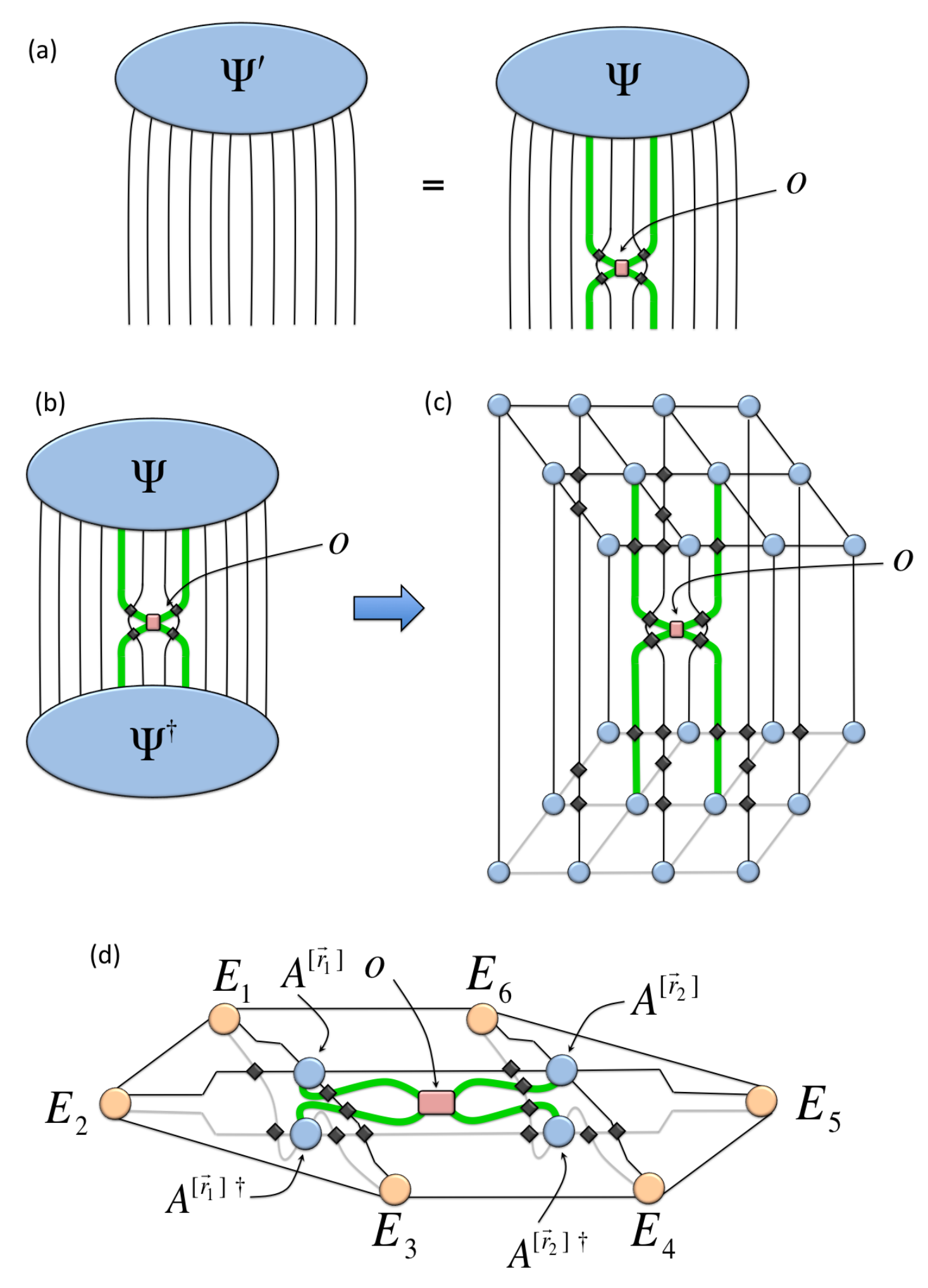
(ii) Local operators. A local fermionic operator $\hat{o}$ is characterized by a tensor of components that describes the action of $\hat{o}$ on a given basis of states. For instance, in the simple case where each site has a vector space $\mathbb{V}$ of dimension $d=2$, we expand a two-site operator $\hat{o}$ as

where

and $\hat{a}$ and $\hat{b}$ are the annihilation operators acting on the two sites (see appendix A for the $d>2$ case). The coefficients $o_{i_{2}i_{1}j_{1}j_{2}}$ are given by

For instance, a hopping term $\hat{a}^{\dagger}\hat{b}$ reads

since the only non-vanishing coefficient is

which is obtained using the anticommutation relations. When the two-site operator $\hat{o}$ acts on two sites $k_{1},k_{2}\in\mathcal{L}$, the state $|\Psi\rangle$ of the system is modified into some other state $\mbox{$|\Psi^{\prime}\rangle$}=\hat{o}\mbox{$|\Psi\rangle$}$. This is implemented simply by connecting the tensor (or tensor network) that represents $\Psi_{s_{1}s_{2}\cdots s_{N}}$ with the four-index tensor $o_{s_{k_{2}}s_{k_{1}}s^{\prime}_{k_{1}}s^{\prime}_{k_{2}}}$ as indicated in Fig. 8(a). In particular, when the two sites are not contiguous in the fermionic order, $|k_{2}-k_{1}|>1$, a number of line crossings appear. This is reflected in the computation of the expectation value $\mbox{$\langle\Psi|$}\hat{o}\mbox{$|\Psi\rangle$}$, see Fig. 8(b)-(d).

(iii) Parity changing tensors. Parity preserving tensors allow us to represent both states $|\Psi\rangle$ with even fermionic particle number (i.e. parity $p=1$) and local operators $\hat{o}$ that are parity preserving. But they also allow us to represent states with an odd fermionic particle number (parity $p=-1$) and parity changing operators. This is so because a parity changing tensor $\tilde{T}$,

can be represented as a parity preserving tensor $T$,

where the additional index $j$ only takes one value, $j=(p,\alpha^{p})=(-1,1)$. For instance, in order to represent a state $\mbox{$|\Psi\rangle$}\in\mathbb{V}^{\otimes N}$ with an odd number of particles by means of a PEPS, an additional index $j=(-1,1)$ is attached to one of the PEPS tensors, see Fig. 9(a). Similarly, a fermionic annihilation operator $c$, which changes parity, can be represented as a tensor with three indices, one of which is fixed to $j=(p,\alpha^{p})=(-1,1)$, see Fig. 9(b). It is sometimes computationally convenient (e.g. in the computation of two-point correlators, Fig. 16) to represent a parity preserving operator that is the product of two parity changing operators, such as the hopping operator $\hat{a}^{\dagger}\hat{b}$ in Eq. (30), by two parity preserving tensors connected by a fixed index $j=(-1,1)$, see Fig. 9(b).

(iv) Simplification. In the particular case of a pair of crossing lines $i$ and $j$ where index $j$ only takes one possible value $p$ of the parity, the fermionic swap gate $\hat{X}$ reduces to a product of two gates. Namely, to a product of two identity operators $\hat{I}\otimes\hat{I}$ if $p=+1$, and to a product of the parity $\hat{P}$ on line $i$ and identity $\hat{I}$ on line $j$ if $p=-1$. It follows, for instance, that the jump move applied to a line $i$ and a parity preserving tensor $T$ with an index $j=(p,\alpha^{p})=(-1,1)$ (used e.g. to represent a parity changing tensor $\tilde{T}$ in Eqs. (33)-34) allows us to ignore index $j$ in $T$ at the price of applying the parity operator $\hat{P}$ to line $i$, see Fig. 10(b). This simplification appears to be useful e.g. in the calculation of the expectation value $\mbox{$\langle\Psi|$}\hat{a}^{\dagger}\hat{b}\mbox{$|\Psi\rangle$}$, see Fig. 16.

A fermionic tensor network can be manipulated simply by performing a sequence of tensor multiplications. It turns out, however, that by considering a special property (jump move) of fermionic tensor networks obeying Rules 1 and 2, the fermionic swap gates can be treated in a very special and advantageous way: they can be ignored until they correspond to a crossing of two indices connected to the same tensor, in which case they can be absorbed into the tensor using a low cost operation. As a result, in a fermionic tensor network algorithm we can follow the same sequence of tensor multiplications that we would have employed to manipulate its bosonic counterpart. In particular, we can use the same optimal sequence of contractions, with the same computational cost (to leading order). Let us discuss all these aspects in more detail.

(i) Jump move. It follows from Rules 1 and 2 that in a fermionic tensor network, as in the bosonic case, lines can be dragged over tensors, see Fig. 10(a). This invariance under ‘jump’ moves allows us to modify fermionic tensor networks in such a way that the fermionic swap gates do not increase the leading cost of manipulations. For a proof of this property, which exploits the fact that tensors are parity-preserving, we refer again to Ref. 12. Notice that the jump move does not include dragging a line over the open end of another line (this would amount to a change in the local fermionic order). The latter transformation is only allowed when it involves a set of open lines with even overall parity, as explained next.

(ii) Open lines. By construction, line ends only appear in the diagrams grouped in such a way that they could be connected to a parity preserving tensor (that is, their combined parity is always even) without introducing additional crossings to the network. For instance, the set of all open legs of the PEPS in Figs. 6(a) or 9(a) have even overall parity, since the PEPS as a whole has parity $p=+1$. Another example is given by the open legs of an environment, Fig. 14(c). Since such groups of open legs with even overall parity could be connected to a parity preserving tensor, the jump move extends naturally to them, as illustrated in Fig. 10(c).

(iii) Absorption of a fermionic swap gate. Given a tensor $T$, with coefficients $T_{i_{1}\cdots ij\cdots i_{M}}$, such that the two contiguous indices $i,j$ are connected to a fermionic swap gate, it is possible to absorb the latter into the former and produce a new tensor $\tilde{T}$ with coefficients

The cost of the absorption is thus just proportional to the number of coefficients in $T$ and comparable to permuting two adjacent indices in a bosonic tensor network. This cost is, in particular, smaller than the tensor multiplication that may have produced $T$ or a subsequent tensor multiplication involving $\tilde{T}$. Therefore the absorption of fermionic swap gates only makes a sub-leading contribution to the total cost of contracting a fermionic tensor network (in the same way that the permutation of indices only makes a sub-leading contribution to the total cost of contracting a bosonic tensor network).

(iv) Same leading cost. In a bosonic system, the contraction of a tensor network is implemented by a sequence of multiplications of tensors, where each multiplication involves two tensors and the sequence is chosen carefully to minimize computational costs. In the fermionic case, it is natural to ask whether the presence of fermionic swap gates will modify the optimal sequence of tensor multiplications and increase the computational cost of the contraction. It turns out that one can always follow the same sequence of multiplications as in the bosonic case. Indeed, as illustrated in the example of Fig. 11, in order to multiply two tensors, one can use jump moves and fermionic swap gate absorptions to eliminate any fermionic swap gate between the two tensors, which can then be multiplied together exactly as in the bosonic case. The leading cost of these manipulations is given by tensor multiplications, and it is therefore the same for bosonic and fermionic systems.

We have explained how to build a fermionic PEPS for the state $\mbox{$|\Psi\rangle$}\in\mathbb{V}^{\otimes N}$ of a fermionic lattice system. The next step is to consider algorithms to compute the expectation value $\langle\hat{o}\rangle$ of a local operator $\hat{o}$ from a fermionic PEPS, as well as to optimize the coefficients in its tensors $\{A^{[\vec{r}]}\}$. It turns out that these algorithms can be obtained by just introducing simple modifications to existing bosonic PEPS algorithms. Here we discuss these modifications broadly.

Let us consider first the computation of the scalar product $\langle\Psi|\Psi\rangle$. As we did in the bosonic case, see Fig. 2, we build this scalar product by connecting the open indices of a PEPS for $|\Psi\rangle$ with those for a PEPS for $\langle\Psi|$ obtained by Hermitian conjugation. The resulting tensor network may contain, in the fermionic case, a large number of fermionic swap gates. However, an important point is that, by using the jump move of Fig. 10(a), the scalar product $\langle\Psi|\Psi\rangle$ can again be re-expressed in terms of a tensor network $\mathcal{E}$ made of reduced tensors $\{a^{[\vec{r}]}\}$, see Fig. 6(d).

As shown in Fig. 6(e), the fermionic reduced tensor $a^{[\vec{r}]}$ differs from its bosonic counterpart by the presence of four fermionic swap gates. Importantly, in a finite or infinite lattice with open boundary conditions, all fermionic swap gates present in the scalar $\langle\Psi|\Psi\rangle$ are absorbed into the reduced tensor $a^{[\vec{r}]}$. Thus, the tensor network $\mathcal{E}$ contains no fermionic swap gates. As a result, an approximation to the scalar product $\langle\Psi|\Psi\rangle$ can be obtained by contracting $\mathcal{E}$ with exactly the same approximate contraction techniques (namely MPS techniques for finite PEPS[15] and either infinite MPS or CTM techniques for infinite PEPS[17, 20]) as in the bosonic case. [In some implementations, it is possible to lower computational costs by considering the components $A^{[\vec{r}]}$ and $A^{[\vec{r}]\dagger}$ of $a^{[\vec{r}]}$ separately. In this case the approximate contraction techniques have to be slightly modified so as to account for the four fermionic swap gates involved in the definition of $a^{[\vec{r}]}$].

Figure 12 considers a PEPS for a fermionic lattice system on a cylinder. Its scalar product can again be expressed in terms of a tensor network $\mathcal{E}$, made of reduced tensors $\{a^{[\vec{r}]}\}$, that contains no line crossings. Therefore its contraction can also be performed exactly as in the bosonic case. Instead, in a fermionic lattice system on a torus, the analogous tensor network $\mathcal{E}$ contains a number of fermionic swap gates, see Fig. 13. However, it can be seen that even in this case $\mathcal{E}$ can still be coarse-grained using the same TERG techniques of Ref. 18, 19 for the bosonic case, by properly coarse-graining the swap fermionic gates at each step of the coarse-graining.

As discussed in Sec. II.3, given an environment $\mathcal{E}^{[\vec{r}_{1}\vec{r_{2}}]}$, an approximation $\mathcal{G}^{[\vec{r}_{1}\vec{r_{2}}]}$ can be used both for the computation of the expectation value $\langle\hat{o}\rangle$ of a local operator $\hat{o}$ and for the optimization of the tensors $\{A^{[\vec{r}]}\}$ defining the PEPS. The approximate contraction of $\mathcal{E}^{[\vec{r}_{1}\vec{r_{2}}]}$ leading to $\mathcal{G}^{[\vec{r}_{1}\vec{r_{2}}]}$ is very similar to the contraction of $\mathcal{E}$ for the scalar product $\langle\Psi|\Psi\rangle$, and can again be accomplished in the fermionic case using the same techniques than in the bosonic case.

From $\mathcal{G}^{[\vec{r}_{1}\vec{r_{2}}]}$, obtaining an approximation to the expectation value $\mbox{$\langle\Psi|$}\hat{o}\mbox{$|\Psi\rangle$}$ involves contracting the tensor network of Fig. 8(d), which differs from its bosonic counterpart in the presence of 12 fermionic swap gates. An analogous tensor network is central to the update of the PEPS tensors $\{A^{[\vec{r}]}\}$ during an imaginary-time evolution towards the ground state $|\Psi_{\mbox{\tiny GS}}\rangle$ of a nearest neighbor fermionic Hamiltonian $\hat{H}$, cf. Eq. (8). More details of this update will be provided in Sec. III in the context of an infinite lattice system, where also the computation of two-point correlators between distant sites will be addressed.

To summarize, the differences between bosonic and fermionic PEPS algorithms are in practice reduced to: (i) use of parity preserving tensors $\{A^{[\vec{r}]}\}$ to efficiently encode the state $\mbox{$|\Psi\rangle$}\in\mathbb{V}^{\otimes N}$; and (ii) presence of fermionic swap gates in some of the tensor networks that need to be contracted, e.g. in order to compute the expected value of a local observable or optimize the tensors $\{A^{[\vec{r}]}\}$ of the variational ansatz. However, thanks to the jump move, the optimal sequence of tensor multiplications involved in the contraction of a given fermionic tensor network is the same than in the bosonic case, as is the incurred computational cost. All in all, we see that fermionic PEPS algorithms can be obtained by introducing a few modifications to bosonic PEPS algorithms. This is further illustrated in the next section, where we provide more details on the specific PEPS algorithm used in Sec. IV, namely the iPEPS algorithm.[17, 20]

The iPEPS ansatz exploits translation invariance of a system on an infinite lattice $\mathcal{L}$ to store the state $|\Psi\rangle$ using only a small number of PEPS tensors, which are repeated throughout the lattice. Here we consider an infinite square lattice $\mathcal{L}$ and assume that the ground state of the system is invariant under translations by one site. We use an iPEPS made of copies of two tensors $A$ and $B$ that are distributed according to a checkerboard pattern, that is,

The reason to use two different tensors $A$ and $B$, instead of a single tensor copied on all locations (as one would expect for a translation invariant ground state) is that the iPEPS algorithm[17, 20] requires that translation invariance be partially broken to the above checkerboard pattern during intermediate stages of the optimization of the ansatz. Invariance under translations by one site is (approximately) restored at the end of the optimization. Needless to say, the same ansatz is also valid for systems where the ground state has checkerboard order (invariance by diagonal shifts), as will be the case in some of the results in Sec. IV.

Let us first consider how to compute the expectation value of a two-site operator $\hat{o}$, see Eq. (2). This requires computing both $\langle\Psi|\Psi\rangle$ and $\mbox{$\langle\Psi|$}\hat{o}\mbox{$|\Psi\rangle$}$.

The scalar product $\langle\Psi|\Psi\rangle$ is expressed in terms of an infinite 2D tensor network $\mathcal{E}$ of reduced tensors $a$ and $b$ distributed according to a checkerboard pattern. As in a finite system, an environment $\mathcal{E}^{[\vec{r}_{1}\vec{r}_{2}]}$ for two nearest sites $\vec{r}_{1},\vec{r}_{2}\in\mathcal{L}$ is then built from $\mathcal{E}$ by removing two reduced tensors, see Fig. 14(a)-(b). Contracting $\mathcal{E}^{[\vec{r}_{1}\vec{r}_{2}]}$ requires an approximation scheme, which produces an approximate environment $\mathcal{G}^{[\vec{r}_{1}\vec{r}_{2}]}$ consisting of six tensors $\{E_{\alpha}\}$ connected through bond indices that take $\chi$ different values, see Fig. 14(d). Here $\chi$ quantifies the degree of approximation in $\mathcal{G}^{[\vec{r}_{1}\vec{r}_{2}]}$. One possible approximation scheme consists in using infinite MPS techniques, as was discussed in the original iPEPS algorithm in Ref. 17. Another possible approximation scheme consists in using CTM techniques,[27] as discussed in the context of the iPEPS algorithm in Ref. 20.

An approximation $\langle\hat{o}\rangle_{\chi}$ to the expectation value $\langle\hat{o}\rangle$ of a two-site observable $\hat{o}$ is then obtained by computing

where $\hat{I}$ denotes the identity operator on the space $\mathbb{V}\otimes\mathbb{V}$ of two sites of $\mathcal{L}$ and we use the same approximate environment $\mathcal{G}^{[\vec{r}_{1}\vec{r}_{2}]}$ to compute $\mbox{$\langle\Psi|$}\hat{o}\mbox{$|\Psi\rangle$}_{\chi}$ and $\mbox{$\langle\Psi|$}\hat{I}\mbox{$|\Psi\rangle$}_{\chi}=\mbox{$\langle\Psi|\Psi\rangle$}_{\chi}$, where the latter is computed as an expectation value for $\hat{o}=\hat{I}$. The approximate value $\langle\hat{o}\rangle_{\chi}$ will in general differ from the exact value $\langle\hat{o}\rangle$. One expects, however, that in the limit of a large $\chi$ one recovers the exact value,

In practice, we compute $\langle\hat{o}\rangle_{\chi}$ for increasingly large values of $\chi$, e.g. $\chi\in\{10,20,\cdots,100\}$, until the expectation value $\langle\hat{o}\rangle_{\chi}$ does no longer depend substantially in $\chi$, and assume that this corresponds to $\langle\hat{o}\rangle$. The cost of computing $\langle\hat{o}\rangle_{\chi}$ using CTM techniques scales with the PEPS bond dimension $D$ and the environment bond dimension $\chi$ as $O(D^{6}\chi^{3})$.

Notice that for any value of the bond dimension $D$, a PEPS produces a variational energy $\langle\hat{H}\rangle$,

that is $\langle\hat{H}\rangle\geq E_{\mbox{\tiny exact}}$, where $E_{\mbox{\tiny exact}}$ is the exact ground state energy. Therefore, if we could compute $\langle\hat{H}\rangle$ exactly, we would obtain an upper bound to $E_{\mbox{\tiny exact}}$, which could e.g. be compared with another upper bound corresponding to another variational ansatz. However, the approximate value $\langle\hat{H}\rangle_{\chi}$ is not guaranteed to be an upper bound to $E_{\mbox{\tiny exact}}$. In this paper we assume that $\langle\hat{H}\rangle_{\chi}$ is an upper bound to $E_{\mbox{\tiny exact}}$ once it has converged for large values of $\chi$. This assumption is seen to be correct in the case of free fermions in Sec. IV.

In the iPEPS algorithm of Refs. 17, 20 an approximation to the ground state is obtained by simulating an evolution in imaginary time, Eq. (8). The optimization of tensors $A$ and $B$ during the imaginary-time evolution is achieved by breaking the evolution into steps (Suzuki-Trotter decomposition) and then considering updates that involve a single link. There are four types of updates, corresponding to the four inequivalent links given by the bond indices $u,l,d,r$ of tensor $A$. For each link, new tensors $A^{\prime}$ and $B^{\prime}$ are produced as a result of an optimization that aims to account for the action of a two-site gate $g=exp(-h^{[\vec{r}_{1}\vec{r}_{2}]}\delta t)$ acting on that link. We refer to Refs. 17, 20 for a detailed explanation on how to use the approximate environment $\mathcal{G}^{[\vec{r}_{1}\vec{r}_{2}]}$ to obtain updated tensors $A^{\prime}$ and $B^{\prime}$. The algorithm proceeds by iteratively updating tensors $A$ and $B$ until they converge to some pair of tensors that depend on $\chi$ and the time step $\delta t$. A finite time step $\delta t$ introduces errors in the imaginary-time evolution. A better approximation to the ground state is obtained by gradually reducing $\delta t$ until its value does no longer affect significantly quantities of interest (e.g. the energy). For instance, this occurs for $\delta t=10^{-5}$ in the simulations of Sec. IV. The cost of simulating an imaginary-time evolution is proportional to the number of time steps that are being simulated and scales as $O(\chi^{3}D^{6})$, since each update requires reconverging an approximate two-site environment $\mathcal{G}^{[\vec{r}_{1}\vec{r}_{2}]}$.

A simplified way of simulating an evolution in imaginary time was proposed in Ref. 19. This simplified update does not involve the environment $\mathcal{G}^{[\vec{r}_{1}\vec{r}_{2}]}$ and has a much lower cost per iteration, namely $O(D^{4}d^{4}+D^{7}d^{3})$ when applied in a straightforward way and reducible to $O(D^{2}d^{6}+D^{3}d^{4}+D^{5}d^{2})$ after more careful considerations. On the one hand, ignoring the environment (that is, the rest of the wavefunction) implies that the update may not be optimal, and indeed there are cases, such as the 2D quantum Ising model near its critical point, where it produces a less accurate approximation to the ground state,[28] although we also found many cases where it only performs marginally worse than when using the environment. On the other hand, its much lower cost accelerates the simulations considerably. Notice, however, that the computation of expectation values with the resulting PEPS still requires computing $\mathcal{G}^{[\vec{r}_{1}\vec{r}_{2}]}$, which has cost $O(\chi^{3}D^{6})$.

As in the bosonic case, the fermionic iPEPS ansatz exploits translation invariance of a system on an infinite lattice $\mathcal{L}$ to store the state $|\Psi\rangle$ using only a small number of PEPS tensors, which are repeated throughout the lattice. Whether we are interested in approximating a ground state invariant under translations by one site or with checkerboard order, we consider again just two (parity preserving) PEPS tensors $A$ and $B$ as in Eq. (36).

It may not seem obvious that a fermionic iPEPS, characterized by tensors $A$ and $B$, represents a state $|\Psi\rangle$ of the infinite lattice $\mathcal{L}$ that is invariant under diagonal shifts (checkerboard order). Indeed, the presence of the ubiquitous fermionic swap gates, which are not homogeneously distributed across the tensor network corresponding to the iPEPS (see Fig. 6 for an illustration in the case of a finite PEPS) may seem incompatible with the checkerboard order. However, the checkerboard order becomes manifest during the computation of expectation values for local observables.

Given a fermionic iPEPS, the computation of the expectation value of e.g. a two-site observable $\hat{o}$ is very similar to the bosonic case. Since there are no fermionic swap gates in the tensor network $\mathcal{E}$ for the scalar product $\langle\Psi|\Psi\rangle$ or the two site environment $\mathcal{E}^{[\vec{r}_{1}\vec{r}_{2}]}$, these tensor networks can be contracted exactly in the same way as in a bosonic iPEPS. [If one wants to use the decomposition of the reduced tensors $a$ and $b$ in terms of $A$ and $B$, Fig. 15, the presence of four fermionic swap gates needs to be taken into account]. In the simulations of Sec. IV, we have used the directional CTM approach discussed in Ref. 20 in order to produce an approximate environment $\mathcal{G}^{[\vec{r}_{1}\vec{r}_{2}]}$. Then an approximation $\langle\hat{o}\rangle_{\chi}$ to the expected value $\langle\hat{o}\rangle$ is computed using the tensor network of Fig. 16(a). Figure 16(b) describes the tensor network that needs to be contracted in order to compute a two-point correlators.

The simulation of time evolution proceeds in a very similar way as in the bosonic iPEPS algorithm, with the difference that the tensor networks involved contain fermionic swap gates instead of simple line crossings. A detailed description of the two updates used in this paper is presented in appendix. B.

Before we move to presenting the results of ground state computations, we conclude this section with a summary of the fermionic iPEPS algorithm:

(i) Ansatz. The state $|\Psi\rangle$ of the system on an infinite square lattice $\mathcal{L}$ is encoded in two parity symmetric tensors $A$ and $B$. These tensors depend on $O(dD^{4})$ parameters, where $d$ is the dimension of the vector space $\mathbb{V}$ of one site of $\mathcal{L}$ and $D$ is the bond dimensions of the iPEPS.

(ii) Computation of expectation values. Given tensors $A$ and $B$, the reduced tensors $a$ and $b$ are computed according to Fig. 15. From the reduced tensors $a$ and $b$, an approximation $\mathcal{G}^{[\vec{r}_{1}\vec{r}_{2}]}$ to a two-site environment $\mathcal{E}^{[\vec{r}_{1}\vec{r}_{2}]}$ is obtained using the CTM algorithm, see Fig. 14. The computational cost scales as $O(\chi^{3}D^{6})$, where $\chi$ is the bond dimension of the approximate environment. Then expectation values are computed by contracting small tensor networks involving $\mathcal{G}^{[\vec{r}_{1}\vec{r}_{2}]}$. For instance, an approximation $\langle\hat{o}\rangle_{\chi}$ to the expected value $\langle\hat{o}\rangle$, Eq. (37), for an operator $\hat{o}$ on two nearest neighbor sites is obtained according to Fig. 16(a), whereas an approximation to a two-point correlator is obtained according to Fig. 16(b).

(iii) Approximation of the ground state. Starting from e.g. random tensors $A$ and $B$, an imaginary-time evolution is used to find an approximation to the ground state of a local Hamiltonian $\hat{H}$. The two updates of appendix B can be used: the standard update, which in general produces better ground state approximations and has cost $O(\chi^{3}D^{6})$; and the simplified update, which has a significantly lower cost and is often only marginally less accurate than the standard update.

References

- [1] J. Hubbard, Proc. Roy. Soc. (London), Ser. A 276, 238 (1963).
- [2] P. W. Anderson, Science 235, 1196 (1987).
- [3] M. Troyer and U.-J. Wiese, Phys. Rev. Lett. 94, 170201 (2005).
- [4] S. R. White, Phys. Rev. Lett. 69, 2863 (1992).
- [5] T. Maier, M. Jarell, T. Pruschke, and M. H. Hettler, Rev. Mod. Phys. 77, 1027 (2005).
- [6] S. Sorella, G. B. Martins, F. Becca, C. Gazza, L. Capriotti, A. Parola, and E. Dagotto, Phys. Rev. Lett. 88, 117002 (2002).
- [7] J. F. Corney and P. D. Drummond, Phys. Rev. Lett. 93, 260401 (2004).
- [8] N.V. Prokof’ev and B.V. Svistunov, Phys. Rev. Lett. 81, 2514 (1998).
- [9] P. Corboz, G. Evenbly, F. Verstraete, and G. Vidal, Phys. Rev. A 81, 010303(R) (2010).
- [10] C. V. Kraus, N. Schuch, F. Verstraete, and J. I. Cirac, arXiv:0904.4667.
- [11] C. Pineda, T. Barthel, and J. Eisert, arXiv:0905.0669.
- [12] P. Corboz and G. Vidal, Phys. Rev. B 80, 165129 (2009).
- [13] T. Barthel, C. Pineda, and J. Eisert, arXiv:0907.3689.
- [14] Q.-Q. Shi, S.-H. Li, J.-H. Zhao, and H.-Q. Zhou, arXiv:0907.5520.
- [15] F. Verstraete and J. I. Cirac, cond-mat/0407066; V. Murg, F. Verstraete, and J. I. Cirac, Phys. Rev. A 75, 033605 (2007).
- [16] G. Sierra and M. A. Martín-Delgado, arXiv:cond-mat/9811170; T. Nishino and K. Okunishi, J. Phys. Soc. Jpn 67 3066 (1998); Y. Nishio, N. Maeshima, A. Gendiar, and T. Nishino, cond-mat/0401115.
- [17] J. Jordan, R. Orús, G. Vidal, F. Verstraete, and J. I. Cirac, Phys. Rev. Lett. 101, 250602 (2008).
- [18] Z.-C. Gu, M. Levin, and X.-G. Wen, Phys. Rev. B 78, 205116 (2008)
- [19] H. C. Jiang, Z. Y. Weng, and T. Xiang, Phys. Rev. Lett. 101, 090603 (2008). Z. Y. Xie, H. C. Jiang, Q. N. Chen, Z. Y. Weng, and T. Xiang, Phys. Rev. Lett. 103, 160601 (2009). P.-C. Chen, C.-Y. Lai, and M.-F. Yang, J. Stat. Mech.: Theory Exp. (2009) P10001.
- [20] R. Orús and G. Vidal, Phys. Rev. B 80, 094403 (2009).
- [21] G. Vidal, Phys. Rev. Lett. 99, 220405 (2007). G. Vidal, Phys. Rev. Lett. 101, 110501 (2008). L. Cincio, J. Dziarmaga, and M. M. Rams Phys. Rev. Lett. 100, 240603 (2008). G. Evenbly and G. Vidal, Phys. Rev. Lett. 102, 180406 (2009). G. Evenbly and G. Vidal, Phys. Rev. B 79, 144108 (2009).
- [22] V. Murg, F. Verstraete, and J. I. Cirac, Phys. Rev. B 79, 195119 (2009).
- [23] G. Evenbly and G. Vidal, arXiv:0904.3383.
- [24] B. Bauer, G. Vidal, and M. Troyer, J. Stat. Mech.: Theory Exp. (2009) P09006.
- [25] P. Chen, C.-Y. Lai, and M.-F. Yang, arXiv:0910.5081.
- [26] F. Verstraete, private communication, Vienna, January 2008.
- [27] T. Nishino and K. Okunishi, J. Phys. Soc. Jpn. 65, 891 (1996).
- [28] J. Jordan, private communication.
- [29] J. de Woul and E. Langmann. arXiv:0907.1277.
- [30] W. Li, L. Ding, R. Yu, T. Roscilde, and S. Haas, Phys. Rev. B 74, 073103 (2006).
- [31] M. M. Wolf, Phys. Rev. Lett. 96, 010404 (2006).
- [32] D. Gioev and I. Klich, Phys. Rev. Lett. 96, 100503 (2006).
- [33] T. Barthel, M.-C. Chung, and U. Schollwock, Phys. Rev. A 74, 022329 (2006).
- [34] G. Evenbly and G. Vidal, arXiv:0710.0692v2.
- [35] W. R. Czart, S. Robaszkiewicz, and B. Tobijaszewska. Acta Phys. Pol. A 114, 129 (2008).
- [36] R. Orús, A. C. Doherty, and G. Vidal, Phys. Rev. Lett. 102, 077203 (2009).
- [37] H. Yokoyama and M. Ogata. J. Phys. Soc. Jpn. 65, 3615 (1996).
- [38] D. A. Ivanov. Phys. Rev. B 70, 104503 (2004).
- [39] M. Lugas, L. Spanu, F. Becca, and S. Sorella. Phys. Rev. B 74, 165122 (2006).
- [40] L. Spanu, M. Lugas, F. Becca, and S. Sorella. Phys. Rev. B 77, 024510 (2008).
- [41] S. R. White and D. J. Scalapino. Phys. Rev. Lett. 80, 1272 (1998).
- [42] S. R. White and D. J. Scalapino. Phys. Rev. Lett. 81, 3227 (1998).
- [43] S. R. White and D. J. Scalapino. Phys. Rev. B 61, 6320 (2000).
- [44] V. J. Emery, S. A. Kivelson, and H. Q. Lin. Phys. Rev. Lett. 64, 475 (1990).
- [45] C. S. Hellberg and E. Manousakis, Phys. Rev. Lett. 78, 4609 (1997).
- [46] S. Singh, R. Pfeifer, and G. Vidal, arXiv:0907.2994.
- [47] N. Schuch, M. M. Wolf, F. Verstraete, and J. I. Cirac. Phys. Rev. Lett. 100, 040501 (2008).
- [48] A. W. Sandvik and G. Vidal. Phys. Rev. Lett. 99, 220602 (2007).