Correlations between perturbation theory and power corrections
in QCD at zero and finite temperature
Abstract
The duality between QCD perturbative series and power corrections recently conjectured by Narison and Zakharov is analyzed. We propose to study correlations between both contributions as diagnostics tool. A very strong correlation between perturbative and non perturbative contributions is observed for several observables at zero and at finite temperature supporting the validity of the dual description.
Keywords:
Perturbation theory, Condensates, Temperature, Power Corrections, Deconfinement, ,
1 Introduction
The disentanglement between perturbative and non perturbative effects in QCD has been a major enterprise in the last three decades since the sum rules technique was first suggested [1, 2]. While short distance radiative corrections are perturbatively computable and are characterized by a smooth logarithmic dependence on the relevant energy scale, non perturbative effects manifest as a stronger power-like dependence and in terms of vacuum expectation values of local and low dimensional gauge invariant operators. Although the underlying quark-gluon dynamics should determine the relative strength of perturbative and non perturbative contributions unambiguously, up till now these condensates have been treated de facto as independent parameters, unrelated to the first few terms of the perturbative series. During many years renormalons have been viewed as a bridge between perturbative and non perturbative physics (see e.g. Ref. [3, 4] and references therein for a review). In a recent paper Narison and Zakharov [5] have conjectured a quite different scenario, namely a duality between condensates and perturbative contributions. This duality concerns the properties of large order perturbative series which involves an expansion in the strong running coupling constant , and it establishes that they are dual to non perturbative power corrections, i.e. powers of . At the practical level, this means that if one considers a short perturbative series then one should add the leading power correction by hand. Only when one uses long perturbative series there is no reason to add power corrections. The confirmation of this conjecture might pave the way for practical approaches where condensates are required; the need of allowed and forbidden local condensates would be justified because of a lack of a complete perturbative series to all orders. This is quite timely since in many applications at zero temperature and finite temperature the phenomenological need for power corrections involving dimension-2 operators is overwhelming. The zero temperature example par excellence is given by the heavy potential, where the string tension, a dimension-2 object not related to any local gauge invariant operator, appears as the unequivocal signal of confinement. There have been speculations on the appearance of dimension 2 contributions to the average plaquette [6]. Recent lattice calculations [7] computing the average plaquette in lattice field theory up to 20-th order do not yet see the onset of renormalon physics; a mild geometric type perturbative series which successfully reconstructs the full result, is observed instead.
While high momenta at zero temperature probes the theory in the asymptotically free region, we note that a parallel discussion for finite temperature above the deconfinement phase transition might be carried out. However, the explicit breaking of Lorentz invariance triggered by the privileged heat bath reference frame makes the theoretical discussion much more involved [8, 9]. At finite temperature the recent discovery of inverse temperature power corrections from relatively old lattice data becomes evident from plots in and has been quite impressive and rather unexpected. They can effectively be explained by a dimension two condensate, starting from the Polyakov loop [10, 11], the heavy quark-antiquark free energy in [12] as well as the trace anomaly and QCD equation of state in [13, 14, 15] (see also Ref. [16]). Of course, it would be quite interesting to determine whether these thermal power corrections are dual, in the sense of Narison and Zakharov, to a long perturbative series. The present paper addresses this important issue.
While the duality conjecture might eventually be tested more convincingly in the future, we suggest an alternative approach where some quantitative insight may also be gathered both at zero and finite temperature from confronting current lattice and perturbative results. Basically, the idea is quite simple. Given that the only scale entering the perturbative series to any order is , in a fit to lattice data containing both perturbation theory and condensates we should observe 1) smaller contributions from condensate at increasing perturbative orders and 2) a rather strong statistical correlation between and the dimensionful condensates.
In the present paper we pursue this idea to check with the accessible theoretical information and lattice data the validity of the duality conjecture. In Sec. 2 we deal first with the more familiar quark-antiquark potential at zero temperature, where we indeed observe, within uncertainties, the expected correlations. This not only supports the perturbative-power duality but also qualifies the correlation method as a handy tool to study the duality elsewhere. We are interested to do so at finite temperature above the deconfinement phase transition for the Polyakov loop in Section 3 and the trace anomaly in Section 4. As a useful guideline we use the finite temperature model where non perturbative thermal power corrections are driven by a dimension 2 gluon condensate in the dimensionally reduced theory [10, 11, 12, 13, 14, 15]. While the model might be improved, taken at face value it provides a unified and coherent description of gluodynamics lattice data using the same values of condensates within estimated errors. It therefore provides an ideal playground to search for possible correlations in the sense of the above mentioned duality.
2 The quark-antiquark potential
Our points are best exemplified with the (zero temperature) heavy quark-antiquark potential within a perturbative expansion for which many efforts have been devoted. Nowadays the perturbative series are partially known up to order in the Weyl or temporal gauge, (see Ref. [17] and references therein11 1 See also [18, 19] for a recent complete three loop calculations in Feynman gauge.). In either case it is known that this perturbative computation can only reproduce lattice data at small separations, and fails for . The Cornell potential is a phenomenological version of this potential and it gives a good overall description of the lattice data [20] for all separations. It reads
| (1) |
where is the QCD coupling constant, which is considered as a constant, i.e. no running, and is the string tension term. The Coulomb term corresponds to the leading order in perturbation theory. The linear term follows from quarkonium phenomenology, and it is widely accepted that it cannot follow from a perturbative computation. This leads to the conclusion that the perturbative potential is not complete, and should be extended with a linear term put by hand, i.e.
| (2) |
Because the accepted separation between perturbative and non perturbative contributions, one is tempted to identify the parameters and . In this section it will be shown that this identification might not be correct, in line with Ref. [5], and in fact there is a mixing between power-like corrections and the perturbative series. This means that eventually . In order to provide further convincing evidence that this might happen, we will analyze lattice data for the heavy potential from Ref. [20] using Eqs. (1) and (2).
Two kinds of fits are considered. In the first ones, a distance interval is sought where the perturbative expansion works well. As expected, this corresponds to taking a sufficiently small distance region, namely, . This regime follows from the requirement that the fitted is compatible with zero within errors. The second type of fits use all distances of lattice data, . In both cases an additive constant is allowed in the potential, chosen so that the fit reproduces exactly a point of lattice data at an intermediate distance . It has been checked that the conclusions are unchanged when this parameter is also included in the fit.
| Order | ||||
|---|---|---|---|---|
| Tree Level | 4.99(11) | 0.991 | 0.98 | |
| 1-loop | 3.66(7) | 4.25(6) | 0.974 | 0.20 |
| 2-loop | 4.54(10) | 4.12(6) | 0.978 | 0.79 |
| N3LO [18, 19] | 4.31(13) | 4.07(6) | 0.980 | 0.93 |
| N3LL [17] | 4.19(14) | 3.85(7) | 0.984 | 0.76 |

For the small distance regime, the perturbative series to describes very well by itself the lattice data () and the string tension turns out to be compatible with zero. The fits including all lattice data are summarized in Table 1. The value of tends to decrease (within errors) as higher orders in perturbation theory are included, and this is what would be expected from the scheme of duality between power corrections and perturbation theory.
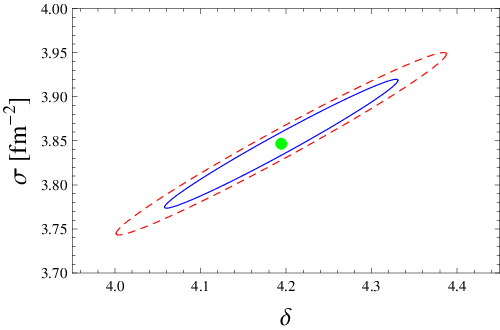
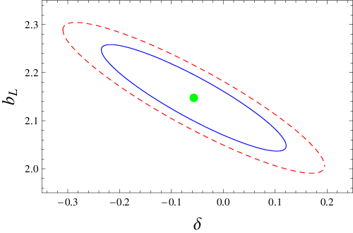
The most relevant feature uncovered by this analysis is the strong correlation found between the perturbative series and the string tension term, not only in the small distance regime, but also in the entire distance regime. Also the correlation is larger at higher orders.22 2 A fit in the interval using the tree level leads to . Figs. 1 and 2 show the correlation ellipses when terms up to N3LL are included in the potential. This strong correlation confirms the dual description of QCD proposed by Narison and Zakharov [5]. In what follows we aim to apply the same correlation method to determine whether or not this duality takes place also at finite temperature above the deconfinement phase transition.
3 The Polyakov loop
The vacuum expectation value of the Polyakov loop in a gauge in which is time independent reads
| (3) |
and an expansion of the exponential gives [10]:
| (4) |
It has been shown in a series of works [10, 11, 12, 13, 14, 15] that power corrections provide the bulk of observables at finite temperature in the non perturbative regime of the deconfined phase of QCD, i.e. in the regime . Our considerations were first proposed to describe the lattice data for the renormalized Polyakov loop in this regime, and follows from the introduction of a tachyonic gluon mass at short distances in the gluon propagator [10]. This is the analog of the zero temperature modification proposed in Ref. [21]. Moreover, as shown in [12], a common value for this mass reproduces both the string tension and Polyakov loop data. These considerations imply that the perturbative value of should be augmented with a non perturbative term directly related to the tachyonic mass [10]:
| (5) |
Up to radiative corrections, the perturbative part is proportional to whereas is temperature independent. Thus, the total Polyakov loop can be separated into perturbative and non perturbative contributions in , and reads ()
| (6) |
The presently available perturbative calculations have been carried out to order [22] (recently corrected in [23]).33 3 For gluodynamics with this gives (7) (where the subindex P stands for perturbative). Since the function starts at order , changes in affect . Clearly, Eq. (6), with a perturbative series plus a dimension 2 power-like term, resembles Eq. (2).
The lattice data from Ref. [24] for the renormalized Polyakov loop with can be fitted using Eq. (6), including the non perturbative term and different orders in the perturbative series. The scale in is taken as . Results are shown in Table 2. Within uncertainties it can be seen that the coefficient of the power-like term does not change much while the correlations are quite strong. The corresponding correlation ellipses are displayed in Fig. 3.
| Order | |||||
|---|---|---|---|---|---|
| 1.121(8) | 1.72(5) | 0.45 | |||
| 1.125(11) | 2.23(16) | 1.22 | |||
| 1.123(9) | 2.15(11) | 1.44 |
The possible contribution of a dimension four condensate in can also be considered. To this end, we carry out a fit with the formula:
| (8) |
The results are shown in Table 3. It is noteworthy that the correlations tend to increase with the perturbative order. Although the fit does not yield a clear signal for , the correlation is remarkably high. This is in line with some appreciation in [5] about the eventual extension of the duality also to dimension four condensates.
4 Trace anomaly and equation of state
Power-like terms have also been found in the equation of state of gluodynamics and QCD [16, 25, 15]. The natural observable to display such effects is the trace anomaly, or interaction measure:
| (9) |
Unlike the pressure, the trace anomaly gets no contribution from the ideal gas part and this is the primary quantity used in lattice to obtain the pressure [26]. Perturbatively, the quantity is proportional to up to radiative corrections. Within the same model used to analyze the Polyakov loop, it has a further power-like contribution proportional to from the dimension 2 condensate [15]:
| (10) |
where is the Debye mass. The trace anomaly can then be expressed in the following form
| (11) |
where for three colors and no quarks. This pattern is similar to the one in Eq. (2) for the potential and in Eq. (6) for the Polyakov loop.
One can make the same analysis that was performed in previous sections, and fit lattice data for the trace anomaly from Ref. [26] using Eq. (11). The weak coupling expansion for the free energy is known up to order [27, 28, 29, 30, 31, 32, 33, 34]. A renormalization group invariant (RGI) resummation, to be used below, is presented in [15]. The perturbative series is poorly convergent for the lattice QCD available temperatures , and even at much higher temperatures. There have also been numerous attempts to resum perturbation theory in order to get a better convergence of the result, one of the most developed techniques being the hard thermal loop (HTL) perturbation theory. The free energy of the gluon plasma has been computed recently up to three-loop order in HTL (see [35] and references therein).
In the fit of the lattice data for the trace anomaly we consider both resummations (RGI and HTL), which enter as the term in Eq. (11). All the fits were performed in a regime in which , so that reliable errors could be extracted. In particular, because PT is expected to work better as the temperature increases, it is sufficient to change the lowest temperature value of the interval. As fitting parameters we take and the parameter defined by . Because the running coupling depends on , a change in is related to a change in , and the correlation between and is measured by the quantity .
| Order | |||||
|---|---|---|---|---|---|
| =const | 3.46(13) | 0.35 | |||
| 3.29(13) | 0.722 | 0.86 | |||
| 3.57(18) | 0.42 | ||||
| 3.73(19) | 0.78 | ||||
| 2.74(58) | 0.891 | 0.99 | |||
| 3.35(49) | 0.983 | 0.37 |
In the RGI resummation, at order an undetermined parameter, , appears due to infrared divergences. Setting , we fit the lattice data using and as free parameters at order . In this case, the best fit in the regime gives [15]:
| (12) |
with . Next we fit and from to . For the highest order the central value of previously obtained is used. The results are shown in Table 4 and Fig. 4. The fit favors vanishing small perturbative contributions, producing large values of . To prevent this, from to an upper bound has been set. Although the results are not fully conclusive, in general, the correlation between perturbative and non perturbative terms becomes larger when higher orders in PT are included, and also, the value of the non perturbative coefficient tends to be smaller for the higher orders. The correlation ellipses for are displayed in Fig. 4.
We have also performed the analyses of this section using lattice data from Refs. [36] and [37]. The values of the parameters agree within estimated errors with those quoted here from Ref. [26]. As a rule these alternative lattice data lead to larger errors. For instance, the fit using the lattice data from Ref. [36] in the regime yields , , , , , , for orders from LO to respectively. The decrease of as the PT order in increased is more evident with these data, although they are affected by larger errors. The correlation increases in this case from at LO to at .

In order to extract the possible contribution of a dimension four condensate, we have also considered a fit using the formula:
| (13) |
The results are shown in Table 5. The parameter is compatible with zero, but a high correlation between both non perturbative terms and is displayed, in line with results of Sec. 3. The correlation tends to increase with the perturbative order, as in Table 4. The correlation ellipsoid corresponding to a joint fit of , and is displayed in Fig. 5.
| Order | ||||||
|---|---|---|---|---|---|---|
| =const | 3.7(7) | 0.31 | ||||
| 3.09(51) | 0.747 | 0.80 | ||||
| 0.30 | ||||||
| 0.31 | ||||||
| 2.6(9) | 0.883 | 0.76 | ||||
| 0.983 | 0.960 | 0.29 |

The analogous analysis can be carried out considering for the HTL perturbation theory result at 1-loop [38], 2-loops [39] and 3-loops [35]. The results are presented in Tables 6 and 7.
| Order | |||||
|---|---|---|---|---|---|
| 1-loop | 3.69(40) | 0.975 | 0.36 | ||
| 2-loops | 3.57(28) | 0.949 | 0.41 | ||
| 3-loops | 0.08(5) | 0.977 | 0.67 |
| Order | ||||||
|---|---|---|---|---|---|---|
| 1-loop | 0.932 | 0.29 | ||||
| 2-loops | 3.58(40) | 0.411 | 0.47 | |||
| 3-loops | 0.964 | 0.92 |
A large correlation between and (or ) is found even at 1-loop order. In addition, the effect of a smaller contribution from at increasing perturbative orders is rather clear in the HTL scheme. Once again, the correlation between dimension 2 and dimension 4 condensates turns out to be strong.44 4 The relative small correlation at 2-loops in Table 7 is confirmed when other lattice data are used [36, 37], but this result seems to be anomalous in view of Table 6. Nevertheless at this order a high correlation between and , , is found.
5 Conclusions
We have proposed to study statistical correlations between perturbative series and power corrections when analyzing lattice QCD results as a way to probe quantitatively the duality proposed by Narison and Zakharov in Ref. [5]. We have found that the effects of this duality start feeling at leading order in perturbation theory, because even at this order the correlations are very strong. We have performed an analysis for the heavy potential at zero temperature, and for several observables in the deconfined regime of thermal QCD, for which power corrections were derived in previous works. As a byproduct, we have addressed the important question on the finding of inverse power corrections at finite temperature above the deconfinement phase transition. Our analysis dissolves the apparent contradiction between the real existence of thermal power corrections in the lattice results and the persistent failure of perturbation theory to a given finite order to reproduce them; these two extremely disjoint scenarios are actually complementary and strongly interrelated.
The present correlation study can be extended to other cases where the condensate-perturbative duality might be expected. A very extreme situation corresponds to just use power corrections and no perturbation theory at all. This could be considered the starting point of the analysis, where some “non perturbative” physics would be expected. Another extreme situation requires a complete knowledge of perturbation theory to all orders, a certainly unrealistic situation. For the situation in-between note that to observe a decreasing condensate for increasing orders in perturbation theory it is not at all trivial as it depends on the behavior of the perturbative expansion. On the other hand, showing that the residual condensate actually vanishes when all terms in perturbation theory are taken into account seems to us as difficult as solving QCD exactly.
We acknowledge useful correspondence with the authors of Ref. [17].
References
- [1] M.A. Shifman, A.I. Vainshtein and V.I. Zakharov, Nucl. Phys. B147 (1979) 385.
- [2] M.A. Shifman, A.I. Vainshtein and V.I. Zakharov, Nucl. Phys. B147 (1979) 448.
- [3] V.I. Zakharov, Prog. Theor. Phys. Suppl. 131 (1998) 107, hep-ph/9802416.
- [4] V.I. Zakharov, (2003), hep-ph/0309178.
- [5] S. Narison and V.I. Zakharov, Phys. Lett. B679 (2009) 355, 0906.4312.
- [6] G. Burgio et al., Phys. Lett. B422 (1998) 219, hep-ph/9706209.
- [7] E.M. Ilgenfritz et al., (2009), 0910.2795.
- [8] U. Kraemmer and A. Rebhan, Rept. Prog. Phys. 67 (2004) 351, hep-ph/0310337.
- [9] E. Shuryak, Prog. Part. Nucl. Phys. 62 (2009) 48, 0807.3033.
- [10] E. Megias, E. Ruiz Arriola and L.L. Salcedo, JHEP 01 (2006) 073, hep-ph/0505215.
- [11] E. Megias, E. Ruiz Arriola and L.L. Salcedo, Eur. Phys. J. A31 (2007) 553, hep-ph/0610163.
- [12] E. Megias, E. Ruiz Arriola and L.L. Salcedo, Phys. Rev. D75 (2007) 105019, hep-ph/0702055.
- [13] E. Megias, E. Ruiz Arriola and L.L. Salcedo, (2008), 0805.4579.
- [14] E. Megias, E.R. Arriola and L.L. Salcedo, Nucl. Phys. Proc. Suppl. 186 (2009) 256, 0809.2044.
- [15] E. Megias, E. Ruiz Arriola and L.L. Salcedo, Phys. Rev. D80 (2009) 056005, 0903.1060.
- [16] R.D. Pisarski, Prog. Theor. Phys. Suppl. 168 (2007) 276, hep-ph/0612191.
- [17] N. Brambilla et al., Phys. Rev. D80 (2009) 034016, 0906.1390.
- [18] C. Anzai, Y. Kiyo and Y. Sumino, (2009), 0911.4335.
- [19] A.V. Smirnov, V.A. Smirnov and M. Steinhauser, (2009), 0911.4742.
- [20] S. Necco and R. Sommer, Nucl. Phys. B622 (2002) 328, hep-lat/0108008.
- [21] K.G. Chetyrkin, S. Narison and V.I. Zakharov, Nucl. Phys. B550 (1999) 353, hep-ph/9811275.
- [22] E. Gava and R. Jengo, Phys. Lett. B105 (1981) 285.
- [23] Y. Burnier, M. Laine and M. Vepsalainen, (2009), 0911.3480.
- [24] S. Gupta, K. Huebner and O. Kaczmarek, Phys. Rev. D77 (2008) 034503, 0711.2251.
- [25] M. Cheng et al., Phys. Rev. D77 (2008) 014511, 0710.0354.
- [26] G. Boyd et al., Nucl. Phys. B469 (1996) 419, hep-lat/9602007.
- [27] E.V. Shuryak, Sov. Phys. JETP 47 (1978) 212.
- [28] S.A. Chin, Phys. Lett. B78 (1978) 552.
- [29] J.I. Kapusta, Nucl. Phys. B148 (1979) 461.
- [30] T. Toimela, Phys. Lett. B124 (1983) 407.
- [31] P. Arnold and C.x. Zhai, Phys. Rev. D51 (1995) 1906, hep-ph/9410360.
- [32] C.x. Zhai and B.M. Kastening, Phys. Rev. D52 (1995) 7232, hep-ph/9507380.
- [33] E. Braaten and A. Nieto, Phys. Rev. D51 (1995) 6990, hep-ph/9501375.
- [34] K. Kajantie et al., Phys. Rev. D67 (2003) 105008, hep-ph/0211321.
- [35] J.O. Andersen, M. Strickland and N. Su, (2009), 0911.0676.
- [36] CP-PACS, M. Okamoto et al., Phys. Rev. D60 (1999) 094510, hep-lat/9905005.
- [37] T. Umeda et al., Phys. Rev. D79 (2009) 051501, 0809.2842.
- [38] J.O. Andersen, E. Braaten and M. Strickland, Phys. Rev. D61 (2000) 014017, hep-ph/9905337.
- [39] J.O. Andersen et al., Phys. Rev. D66 (2002) 085016, hep-ph/0205085.