跳到论文正文
W Papers独立论文阅读器 arXiv:0912.0429 论文正文 计算阅读时间 · 0%
引用这篇论文根据当前论文元数据生成,正式投稿前建议核对。


License: arXiv.org perpetual non-exclusive license
arXiv:0912.0429v1 [math.CO] 02 Dec 2009

Loops in canonical RNA pseudoknot structures

Markus E. Nebel†, Christian M. Reidys∗ and Rita R. Wang ∗ Address: ∗ Center for Combinatorics, LPMC-TJKLC
Nankai University
Tianjin 300071
P.R. China
Phone: *86-22-2350-6800
Fax: *86-22-2350-9272
† TU Kaiserslautern
67663 Kaiserslautern
Germany
Email address: reidys@nankai.edu.cn
Date: October, 2009
Abstract.

In this paper we compute the limit distributions of the numbers of hairpin-loops, interior-loops and bulges in kk-noncrossing RNA structures. The latter are coarse grained RNA structures allowing for cross-serial interactions, subject to the constraint that there are at most k−1k-1 mutually crossing arcs in the diagram representation of the molecule. We prove central limit theorems by means of studying the corresponding bivariate generating functions. These generating functions are obtained by symbolic inflation of 𝗅𝗏k𝟧{\sf lv}_{k}^{\sf 5}-shapes [11].

Key words and phrases: 
kk-noncrossing τ\tau-canonical RNA structure, bivariate generating function, singularity analysis, central limit theorem, hairpin-loop, interior-loop, bulge

1. Introduction

An RNA molecule is a sequence of the four nucleotides A, G, U, C together with the Watson-Crick (A-U, G-C) and U-G base pairing rules. The sequence of bases is called the primary structure of the RNA molecule. Two bases in the primary structure which are not adjacent may form hydrogen bonds following the Watson-Crick base pairing rules. Three decades ago Waterman et al. [9, 10, 13] analyzed RNA secondary structures. Secondary structures are coarse grained RNA contact structures. They can be represented as diagrams and planar graphs, see Fig. 1.

Refer to caption

Figure 1. The Sprinzl tRNA RD7550 secondary structure represented as 22-noncrossing diagram (top) and planar graph (bottom).

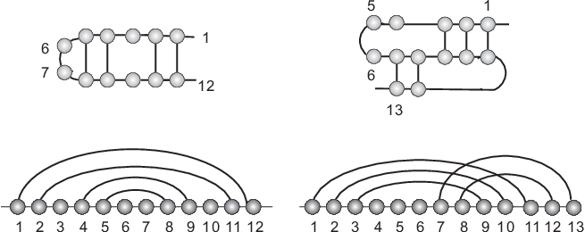
Diagrams are labeled graphs over the vertex set [n]={1,…,n}[n]=\{1,\dots,n\} with vertex degrees ≤1\leq 1, represented by drawing its vertices on a horizontal line and its arcs (i,j)(i,j) (i<ji<j), in the upper half-plane, see Fig. 1 and Fig. 2. Here, vertices and arcs correspond to the nucleotides A, G, U, C and Watson-Crick (A-U, G-C) and (U-G) base pairs, respectively. In a diagram two arcs (i1,j1)(i_{1},j_{1}) and (i2,j2)(i_{2},j_{2}) are called crossing if i1<i2<j1<j2i_{1}<i_{2}<j_{1}<j_{2} holds. Accordingly, a kk-crossing is a sequence of arcs (i1,j1),…,(ik,jk)(i_{1},j_{1}),\dots,(i_{k},j_{k}) such that i1<i2<⋯<ik<j1<j2<⋯<jki_{1}<i_{2}<\dots<i_{k}<j_{1}<j_{2}<\dots<j_{k}, see Fig. 2. We call diagrams containing at most (k−1)(k-1)-crossings, kk-noncrossing diagrams (kk-noncrossing partial matchings). The length of an arc (i,j)(i,j) is given by j−ij-i, characterizing the minimal length of a hairpin loop. A stack of length τ\tau is a sequence of “parallel” arcs of the form

(1.1) ((i,j),(i+1,j−1),…,(i+(τ−1),j−(τ−1))),((i,j),(i+1,j-1),\ldots,(i+(\tau-1),j-(\tau-1))),

and we denote it by Si,jτS_{i,j}^{\tau}. We call an arc of length one a 11-arc. A kk-noncrossing, τ\tau-canonical RNA structure is a kk-noncrossing diagram without 11-arcs, having a minimum stack-size of τ\tau, see Fig. 2. Let 𝒯k,τ​(n)\mathcal{T}_{k,\tau}(n) denote the set of kk-noncrossing, τ\tau-canonical RNA structures of length nn and let 𝖳k,τ​(n)\mathsf{T}_{k,\tau}(n) denote their number.

Refer to caption

Figure 2. A 22-noncrossing, 22-canonical RNA structure (left) and a 33-noncrossing, 22-canonical RNA structure (right) represented as planer graphs (top) and diagrams (bottom).

We next introduce the following structural elements of kk-noncrossing, τ\tau-canonical RNA structures, see Fig. 3 and Fig. 4.

Refer to caption

Figure 3. 33-noncrossing, 66-canonical structures: the pseudoknot structure of the PrP-encoding mRNA represented as diagrams (top) and planer graphs (bottom)..

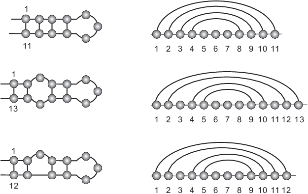
Let [i,j][i,j] denote an interval, i.e. a sequence of consecutive isolated vertices (i,i+1,…,j−1,j)(i,i+1,\ldots,j-1,j). We consider, see Fig. 4

  1. (1)

    a hairpin-loop is a pair

    ((i,j),[i+1,j−1]).((i,j),[i+1,j-1]).
  2. (2)

    an interior-loop is a sequence

    ((i1,j1),[i1+1,i2−1],(i2,j2),[j2+1,j1−1]),((i_{1},j_{1}),[i_{1}+1,i_{2}-1],(i_{2},j_{2}),[j_{2}+1,j_{1}-1]),

    where (i2,j2)(i_{2},j_{2}) is nested in (i1,j1)(i_{1},j_{1}).

  3. (3)

    a bulge is a sequence

    ((i1,j1),[i1+1,i2−1],(i2,j1−1))or((i1,j1),(i1+1,j2),[j2+1,j1−1]).((i_{1},j_{1}),[i_{1}+1,i_{2}-1],(i_{2},j_{1}-1))\quad\text{or}\quad((i_{1},j_{1}),(i_{1}+1,j_{2}),[j_{2}+1,j_{1}-1]).
  4. (4)

    a stem is a sequence of stacks

    (Si1,j1τ1,Si2,j2τ2,…,Sis,jsτs)\left(S_{i_{1},j_{1}}^{\tau_{1}},S_{i_{2},j_{2}}^{\tau_{2}},\ldots,S_{i_{s},j_{s}}^{\tau_{s}}\right)

    where the stack Sim,jmτmS_{i_{m},j_{m}}^{\tau_{m}} is nested in Sim−1,jm−1τm−1S_{i_{m-1},j_{m-1}}^{\tau_{m-1}}, 2≤m≤s2\leq m\leq s and there are no arcs of the form (i1−1,j1+1)(i_{1}-1,j_{1}+1) and (is+τs,js−τs)(i_{s}+\tau_{s},j_{s}-\tau_{s}).

Refer to caption

Figure 4. The loop-types: hairpin-loop (top), interior-loop (middle) and bulge (bottom).

2. Preliminaries

Let fk​(n,ℓ)f_{k}(n,\ell) denote the number of kk-noncrossing diagrams on nn vertices having exactly ℓ\ell isolated vertices. A diagram without isolated points is called a matching. The exponential generating function of kk-noncrossing matchings satisfies the following identity [2, 4, 5]

(2.1) 𝐇k​(z)=∑n≥0fk​(2​n,0)⋅z2​n(2​n)!=det[Ii−j​(2​z)−Ii+j​(2​z)]|i,j=1k−1{{\bf H}_{k}(z)}=\sum_{n\geq 0}f_{k}(2n,0)\cdot\frac{z^{2n}}{(2n)!}=\det[I_{i-j}(2z)-I_{i+j}(2z)]|_{i,j=1}^{k-1}

where Ir​(2​z)=∑j≥0z2​j+rj!​(j+r)!I_{r}(2z)=\sum_{j\geq 0}\frac{z^{2j+r}}{{j!(j+r)!}} is the hyperbolic Bessel function of the first kind of order rr. Eq. (2.1) allows us to conclude that the ordinary generating function

𝐅k​(z)=∑n≥0fk​(2​n,0)​zn{\bf F}_{k}(z)=\sum_{n\geq 0}f_{k}(2n,0)z^{n}

is DD-finite [12]. This follows from the fact that Ir​(2​z)I_{r}(2z) is DD-finite and DD-finite power series form an algebra [12]. Consequently, there exists some e∈ℕe\in\mathbb{N} such that

(2.2) q0,k​(z)​ded​ze​𝐅k​(z)+q1,k​(z)​de−1d​ze−1​𝐅k​(z)+⋯+qe,k​(z)​𝐅k​(z)=0,q_{0,k}(z)\frac{d^{e}}{dz^{e}}{\bf F}_{k}(z)+q_{1,k}(z)\frac{d^{e-1}}{dz^{e-1}}{\bf F}_{k}(z)+\cdots+q_{e,k}(z){\bf F}_{k}(z)=0,

where qj,k​(z)q_{j,k}(z) are polynomials and q0,k​(z)≠0q_{0,k}(z)\neq 0. The ordinary differential equations (ODE) for 𝐅k​(z){\bf F}_{k}(z), where 2≤k≤72\leq k\leq 7 are obtained by the MAPLE package GFUN from the exact data of fk​(2​n,0)f_{k}(2n,0). They are verified by first deriving the corresponding PP-recursions [12] for fk​(2​n,0)f_{k}(2n,0) second transforming these PP-recursions into PP-recursions of fk​(2​n,0)/(2​n)!f_{k}(2n,0)/(2n)! and third deriving the corresponding ODEs for 𝐇k​(z){\bf H}_{k}(z) and verifying that the RHS of eq. (2.1) is a solution. The key point is that any singularity of 𝐅k​(z){\bf F}_{k}(z) is contained in the set of roots of q0,k​(z)q_{0,k}(z) [12], which we denote by RkR_{k}. For 2≤k≤72\leq k\leq 7, we give the polynomials q0,k​(z)q_{0,k}(z) and their roots in Table 1.

kk q0,k​(z)q_{0,k}(z) RkR_{k}
22 (4​z−1)​z(4z-1)z {14}\{\frac{1}{4}\}
33 (16​z−1)​z2(16z-1)z^{2} {116}\{\frac{1}{16}\}
44 (144​z2−40​z+1)​z3(144z^{2}-40z+1)z^{3} {14,136}\{\frac{1}{4},\frac{1}{36}\}
55 (1024​z2−80​z+1)​z4(1024z^{2}-80z+1)z^{4} {116,164}\{\frac{1}{16},\frac{1}{64}\}
66 (14400​z3−4144​z2+140​z−1)​z5(14400z^{3}-4144z^{2}+140z-1)z^{5} {14,136,1100}\{\frac{1}{4},\frac{1}{36},\frac{1}{100}\}
77 (147456​z3−12544​z2+224​z−1)​z6(147456z^{3}-12544z^{2}+224z-1)z^{6} {116,164,1144}\{\frac{1}{16},\frac{1}{64},\frac{1}{144}\}

Table 1. We present the polynomials q0,k​(z)q_{0,k}(z) and their nonzero roots obtained by the MAPLE package GFUN.

In [8] we showed that for arbitrary kk

(2.3) fk​(2​n,0)∼c~k​n−((k−1)2+(k−1)/2)​(2​(k−1))2​n,c~k>0f_{k}(2n,0)\,\sim\,\widetilde{c}_{k}\,n^{-((k-1)^{2}+(k-1)/2)}\,(2(k-1))^{2n},\qquad\widetilde{c}_{k}>0

in accordance with the fact that 𝐅k​(z){\bf F}_{k}(z) has the unique dominant singularity ρk2\rho_{k}^{2}, where ρk=1/(2​k−2)\rho_{k}=1/(2k-2).

We next introduce a central limit theorem due to Bender [1]. It is proved by analyzing the characteristic function by the Lévy-Cramér Theorem (Theorem IX.4 in [3]).

Theorem 1.

Suppose we are given the bivariate generating function

(2.4) f⁡(z,u)=∑n,t≥0f⁡(n,t)​zn​ut,f(z,u)=\sum_{n,t\geq 0}f(n,t)\,z^{n}\,u^{t},

where f⁡(n,t)≥0f(n,t)\geq 0 and f⁡(n)=∑tf⁡(n,t)f(n)=\sum_{t}f(n,t). Let 𝕏n\mathbb{X}_{n} be a r.v. such that ℙ⁡(𝕏n=t)=f⁡(n,t)/f⁡(n)\mathbb{P}(\mathbb{X}_{n}=t)=f(n,t)/f(n). Suppose

(2.5) [zn]​f​(z,es)∼c⁡(s)​nα​γ​(s)−n[z^{n}]f(z,e^{s})\sim c(s)\,n^{\alpha}\,\gamma(s)^{-n}

uniformly in ss in a neighborhood of 00, where c⁡(s)c(s) is continuous and nonzero near 00, α\alpha is a constant, and γ⁡(s)\gamma(s) is analytic near 00. Then there exists a pair (μ,σ)(\mu,\sigma) such that the normalized random variable

(2.6) 𝕏n∗=𝕏n−μ​nn​σ2\mathbb{X}^{*}_{n}=\frac{\mathbb{X}_{n}-\mu\,n}{\sqrt{{n\,\sigma}^{2}}}

has asymptotically normal distribution with parameter (0,1)(0,1). That is we have

(2.7) limn→∞ℙ⁡(𝕏n∗<x)=12​π​∫−∞xe−12​c2​𝑑c\lim_{n\to\infty}\mathbb{P}\left(\mathbb{X}^{*}_{n}<x\right)=\frac{1}{\sqrt{2\pi}}\int_{-\infty}^{x}\,e^{-\frac{1}{2}c^{2}}dc\,

where μ\mu and σ2\sigma^{2} are given by

(2.8) μ=−γ′​(0)γ⁡(0)andσ2=(γ′​(0)γ⁡(0))2−γ′′​(0)γ⁡(0).\mu=-\frac{\gamma^{\prime}(0)}{\gamma(0)}\quad\text{\it and}\quad\sigma^{2}=\left(\frac{\gamma^{\prime}(0)}{\gamma(0)}\right)^{2}-\frac{\gamma^{\prime\prime}(0)}{\gamma(0)}.

The crucial points for applying Theorem 1 are (a) eq. (2.5)

[zn]​f​(z,es)∼c⁡(s)​nα​γ​(s)−n,[z^{n}]f(z,e^{s})\sim c(s)\,n^{\alpha}\,\gamma(s)^{-n},

uniformly in ss in a neighborhood of 00, where c⁡(s)c(s) is continuous and nonzero near 00 and α\alpha is a constant and (b) the analyticity of γ⁡(s)\gamma(s) in ss near 00. In the following, we have generating functions of the form 𝐅k​(ψ​(z,s)){\bf F}_{k}(\psi(z,s)). In this situation, Theorem 2 below guarantees under specific conditions

[zn]​𝐅k​(ψ⁡(z,s))∼A⁡(s)​n−((k−1)2+(k−1)/2)​(1γ⁡(s))n,A⁡(s) continuous,[z^{n}]{\bf F}_{k}(\psi(z,s))\sim A(s)\,n^{-((k-1)^{2}+(k-1)/2)}\left(\frac{1}{\gamma(s)}\right)^{n},\quad\text{$A(s)$ continuous},

for 2≤k≤72\leq k\leq 7. The analyticity of γ⁡(s)\gamma(s) is guaranteed by the analytic implicit function theorem [3].

Theorem 2.

[7] Suppose 2≤k≤72\leq k\leq 7. Let ψ⁡(z,s)\psi(z,s) be an analytic function in a domain

(2.9) 𝒟={(z,s)||z|≤r,|s|<ϵ}\mathcal{D}=\{(z,s)||z|\leq r,|s|<\epsilon\}

such that ψ⁡(0,s)=0\psi(0,s)=0. In addition suppose γ⁡(s)\gamma(s) is the unique dominant singularity of 𝐅k​(ψ​(z,s)){\bf F}_{k}(\psi(z,s)) and analytic solution of ψ⁡(γ⁡(s),s)=ρk2\psi(\gamma(s),s)=\rho_{k}^{2}, |γ⁡(s)|≤r|\gamma(s)|\leq r, ∂zψ⁡(γ⁡(s),s)≠0\partial_{z}\psi(\gamma(s),s)\neq 0 for |s|<ϵ|s|<\epsilon. Then 𝐅k​(ψ​(z,s)){\bf F}_{k}(\psi(z,s)) has a singular expansion and

(2.10) [zn]𝐅k(ψ(z,s))∼A(s)n−((k−1)2+(k−1)/2)(1γ⁡(s))nfor some continuous A⁡(s)∈ℂ,[z^{n}]{\bf F}_{k}(\psi(z,s))\sim A(s)\,n^{-((k-1)^{2}+(k-1)/2)}\left(\frac{1}{\gamma(s)}\right)^{n}\quad\text{for some continuous $A(s)\in\mathbb{C}$},

uniformly in ss contained in a small neighborhood of 00.

To keep the paper selfcontained we give a direct proof of Theorem 2 in Section 5. This avoids calling upon generic results, such as the uniformity Lemma of singularity analysis [3].

3. The generating function

In this section we compute the bivariate generating functions of hairpin-loops, interior-loops and bulges. Let hk,τ​(n,t)h_{k,\tau}(n,t), ik,τ​(n,t)i_{k,\tau}(n,t) and bk,τ​(n,t)b_{k,\tau}(n,t) denote the numbers of kk-noncrossing, τ\tau-canonical RNA structures of length nn with tt hairpin-loops, interior-loops and bulges. We set

(3.1) 𝐇k,τ​(z,u1)\displaystyle{\bf H}_{k,\tau}(z,u_{1}) =\displaystyle= ∑n≥0∑t≥0hk,τ​(n,t)​zn​u1t,\displaystyle\sum_{n\geq 0}\sum_{t\geq 0}h_{k,\tau}(n,t)z^{n}\,u_{1}^{t},
(3.2) 𝐈k,τ​(z,u2)\displaystyle{\bf I}_{k,\tau}(z,u_{2}) =\displaystyle= ∑n≥0∑t≥0ik,τ​(n,t)​zn​u2t,\displaystyle\sum_{n\geq 0}\sum_{t\geq 0}i_{k,\tau}(n,t)z^{n}\,u_{2}^{t},
(3.3) 𝐁k,τ​(z,u3)\displaystyle{\bf B}_{k,\tau}(z,u_{3}) =\displaystyle= ∑n≥0∑t≥0bk,τ​(n,t)​zn​u3t.\displaystyle\sum_{n\geq 0}\sum_{t\geq 0}b_{k,\tau}(n,t)z^{n}\,u_{3}^{t}.

In order to derive the above generating functions we use symbolic enumeration [3]. A combinatorial class is a set of finite size with the definition of size function of its elements, whose elements are all finite size and the number of certain size elements is finite. Suppose 𝒞\mathcal{C} be a combinatorial class and c∈𝒞c\in\mathcal{C}. We denote the size of cc by |c||c|. There are two special combinatorial classes ℰ\mathcal{E} and 𝒵\mathcal{Z} which respectively contains only an element of size 00 and an element of size 11. The subset of 𝒞\mathcal{C} which contains all the elements of size nn in 𝒞\mathcal{C} is denoted by 𝒞n\mathcal{C}_{n}. Then the generating function of a combinatorial class 𝒞\mathcal{C} is

(3.4) 𝐂⁡(z)=∑c∈𝒞z|c|=∑n≥0Cn​zn,{\bf C}(z)=\sum_{c\in\mathcal{C}}z^{|c|}=\sum_{n\geq 0}C_{n}\,z^{n},

where 𝒞n⊂𝒞\mathcal{C}_{n}\subset\mathcal{C} and Cn=|𝒞n|C_{n}=|\mathcal{C}_{n}|. In particular the generating functions of ℰ\mathcal{E} and 𝒵\mathcal{Z} are given by 𝐄⁡(z)=1{\bf E}(z)=1 and 𝐙⁡(z)=z{\bf Z}(z)=z. For any two combinatorial classes 𝒞\mathcal{C}, 𝒟\mathcal{D}, we have the following operations:

  • •

    𝒞+𝒟:=𝒞∪𝒟\mathcal{C}+\mathcal{D}:=\mathcal{C}\cup\mathcal{D}, if 𝒞∩𝒟=∅\mathcal{C}\cap\mathcal{D}=\varnothing

  • •

    𝒞×𝒟:={(c,d)|c∈𝒞,d∈𝒟}\mathcal{C}\times\mathcal{D}:=\{(c,d)|c\in\mathcal{C},d\in\mathcal{D}\} and 𝒞m:=∏i=1m𝒞\mathcal{C}^{m}:=\prod_{i=1}^{m}\mathcal{C}

  • •

    Seq​(𝒞)=ℰ+𝒞+𝒞2+⋯\textsc{Seq}(\mathcal{C})={\mathcal{E}}+\mathcal{C}+\mathcal{C}^{2}+\cdots.

We have the following relations between the operations of combinatorial classes and the operations of their generating functions:

(3.5) 𝒜=𝒞+𝒟\displaystyle\mathcal{A}=\mathcal{C}+\mathcal{D} ⇒\displaystyle\Rightarrow 𝐀⁡(z)=𝐂⁡(z)+𝐃⁡(z)\displaystyle{\bf A}(z)={\bf C}(z)+{\bf D}(z)
(3.6) 𝒜=𝒞×𝒟\displaystyle\mathcal{A}=\mathcal{C}\times\mathcal{D} ⇒\displaystyle\Rightarrow 𝐀⁡(z)=𝐂⁡(z)⋅𝐃⁡(z)\displaystyle{\bf A}(z)={\bf C}(z)\cdot{\bf D}(z)
(3.7) 𝒜=Seq​(𝒞)\displaystyle\mathcal{A}=\textsc{Seq}(\mathcal{C}) ⇒\displaystyle\Rightarrow 𝐀⁡(z)=(1−𝐂⁡(z))−1,\displaystyle{\bf A}(z)=(1-{\bf C}(z))^{-1},

where 𝐀⁡(z){\bf A}(z), 𝐂⁡(z){\bf C}(z), 𝐃⁡(z){\bf D}(z) is the generating function of 𝒜\mathcal{A}, 𝒞\mathcal{C} and 𝒟\mathcal{D}.

Given a kk-noncrossing, τ\tau-canonical RNA structure δ\delta, its 𝗅𝗏k𝟧{\sf lv}_{k}^{\sf 5}-shape, 𝗅𝗏k𝟧​(δ){\sf lv}_{k}^{\sf 5}(\delta) [11], is obtained by first removing all isolated vertices and second collapsing any stack into a single arc, see Fig.5. By construction, 𝗅𝗏k𝟧{\sf lv}_{k}^{\sf 5}-shapes do not preserve stack-lengths, interior loops and unpaired regions. In the following, we shall refer to 𝗅𝗏k𝟧{\sf lv}_{k}^{\sf 5}-shape simply as shape. Let 𝒯k,τ{\mathcal{T}}_{k,\tau} denote the set of kk-noncrossing, τ\tau-canonical structures and ℐk{\mathcal{I}}_{k} the set of all kk-noncrossing shapes and ℐk​(m){\mathcal{I}}_{k}(m) those having mm 11-arcs, see Figure 5. Each stem of a kk-noncrossing, τ\tau-canonical RNA structure is mapped into an arc in its corresponding shape and all hairpin-loops are mapped into 11-arcs. Therefore we have the surjective map,

(3.8) φ:𝒯k,τ→ℐk.\varphi:\ {\mathcal{T}}_{k,\tau}\rightarrow{\mathcal{I}}_{k}.

Refer to caption

Figure 5. A 33-noncrossing, 22-canonical RNA structure (top-left) is mapped into its shape (top-right) in two steps. A stem (blue) is mapped into a single shape-arc (blue). A hairpin-loop (red) is mapped into a shape-11-arc (red).

Indeed, for a given shape γ\gamma in ℐk{\mathcal{I}}_{k}, we can derive a kk-noncrossing, τ\tau-canonical structure having arc-length≥2\geq 2, we can add arcs to each arc contained in the shape such that every resulting stack has τ\tau arcs and insert one isolated vertex in each 11-arc. Let ℐk​(s,m){\mathcal{I}}_{k}(s,m) and ik​(s,m)i_{k}(s,m) denote the set and number of the 𝗅𝗏k𝟧{\sf lv}_{k}^{\sf 5}-shapes of length 2​s2s with mm 11-arcs and

(3.9) 𝐈k​(x,y)=∑s≥0∑m=0sik​(s,m)​xs​ym{\bf I}_{k}(x,y)=\sum_{s\geq 0}\sum_{m=0}^{s}i_{k}(s,m)x^{s}y^{m}

be the bivariate generating function. Furthermore, let ℐk​(m)\mathcal{I}_{k}(m) denote the set of shapes γ\gamma having mm 11-arcs. Let k,s,mk,s,m be natural numbers where k≥2k\geq 2, then the generating function 𝐈k​(x,y){\bf I}_{k}(x,y) [11] is given by

(3.10) 𝐈k​(x,y)=1+x1+2​x−x​y​𝐅k​(x⁡(1+x)(1+2​x−x​y)2){\bf I}_{k}(x,y)=\frac{1+x}{1+2x-xy}{\bf F}_{k}\left(\frac{x(1+x)}{(1+2x-xy)^{2}}\right)
Theorem 3.

Suppose k,τ∈ℕ,k≥2,τ≥1k,\tau\in\mathbb{N},k\geq 2,\tau\geq 1. Then

(3.11) 𝐇k,τ​(z,u1)=(1−z)​(1−z2+z2​τ)(1−z)2​(1−z2+z2​τ)+z2​τ−z2​τ+1​u1𝐅k​(z2​τ​(1−z)2​(1−z2+z2​τ)((1−z)2​(1−z2+z2​τ)+z2​τ−z2​τ+1​u1)2),\begin{split}{\bf H}_{k,\tau}(z,u_{1})=&\frac{(1-z)(1-z^{2}+z^{2\tau})}{(1-z)^{2}(1-z^{2}+z^{2\tau})+z^{2\tau}-z^{2\tau+1}u_{1}}\\ &{\bf F}_{k}\left(\frac{z^{2\tau}(1-z)^{2}(1-z^{2}+z^{2\tau})}{\left((1-z)^{2}(1-z^{2}+z^{2\tau})+z^{2\tau}-z^{2\tau+1}u_{1}\right)^{2}}\right),\end{split}
(3.12) 𝐈k,τ​(z,u2)=(1−z2)​(1−z)2−u2​z2​τ+2+(2​z2−2​z+1)​z2​τ(1−z)​((1−z2)​(1−z)2−u2​z2​τ+2+(2​z2−3​z+2)​z2​τ)𝐅k​(z2​τ​((1−z2)​(1−z)2−u2​z2​τ+2+(2​z2−2​z+1)​z2​τ)((1−z2)​(1−z)2−u2​z2​τ+2+(2​z2−3​z+2)​z2​τ)2),\begin{split}{\bf I}_{k,\tau}(z,u_{2})=&\frac{(1-z^{2})(1-z)^{2}-u_{2}z^{2\tau+2}+(2z^{2}-2z+1)z^{2\tau}}{(1-z)\left((1-z^{2})(1-z)^{2}-u_{2}z^{2\tau+2}+(2z^{2}-3z+2)z^{2\tau}\right)}\\ &{\bf F}_{k}\left(\frac{z^{2\tau}\left((1-z^{2})(1-z)^{2}-u_{2}z^{2\tau+2}+(2z^{2}-2z+1)z^{2\tau}\right)}{\left((1-z^{2})(1-z)^{2}-u_{2}z^{2\tau+2}+(2z^{2}-3z+2)z^{2\tau}\right)^{2}}\right),\end{split}
(3.13) 𝐁k,τ​(z,u3)=(1−z2)​(1−z)−2​u3​z2​τ+1+(z+1)​z2​τ(1−z)​((1−z2)​(1−z)−2​u3​z2​τ+1+(z+2)​z2​τ)𝐅k​(z2​τ​((1−z2)​(1−z)−2​u3​z2​τ+1+(z+1)​z2​τ)(1−z)​((1−z2)​(1−z)−2​u3​z2​τ+1+(z+2)​z2​τ)2).\begin{split}{\bf B}_{k,\tau}(z,u_{3})=&\frac{(1-z^{2})(1-z)-2u_{3}z^{2\tau+1}+(z+1)z^{2\tau}}{(1-z)\left((1-z^{2})(1-z)-2u_{3}z^{2\tau+1}+(z+2)z^{2\tau}\right)}\\ &{\bf F}_{k}\left(\frac{z^{2\tau}\left((1-z^{2})(1-z)-2u_{3}z^{2\tau+1}+(z+1)z^{2\tau}\right)}{(1-z)\left((1-z^{2})(1-z)-2u_{3}z^{2\tau+1}+(z+2)z^{2\tau}\right)^{2}}\right).\end{split}
Proof.

We prove the theorem via symbolic enumeration representing a kk-noncrossing, τ\tau-canonical structure as the inflation of a shape, γ\gamma. Since a structure inflated from γ∈ℐk​(s,m)\gamma\in\mathcal{I}_{k}(s,m) has exactly ss stems, (2​s+1)(2s+1) (possibly empty) intervals of isolated vertices and mm nonempty such intervals we rewrite the generating functions as

𝐇k,τ​(z,u1)\displaystyle{\bf H}_{k,\tau}(z,u_{1}) =\displaystyle= ∑m≥0∑γ∈ℐk​(m)𝐓γ​(z,u1,1,1),\displaystyle\sum_{m\geq 0}\sum_{\gamma\in\,{\mathcal{I}}_{k}(m)}{\bf T}_{\gamma}(z,u_{1},1,1),
𝐈k,τ​(z,u2)\displaystyle{\bf I}_{k,\tau}(z,u_{2}) =\displaystyle= ∑m≥0∑γ∈ℐk​(m)𝐓γ​(z,1,u2,1),\displaystyle\sum_{m\geq 0}\sum_{\gamma\in\,{\mathcal{I}}_{k}(m)}{\bf T}_{\gamma}(z,1,u_{2},1),
𝐁k,τ​(z,u3)\displaystyle{\bf B}_{k,\tau}(z,u_{3}) =\displaystyle= ∑m≥0∑γ∈ℐk​(m)𝐓γ​(z,1,1,u3).\displaystyle\sum_{m\geq 0}\sum_{\gamma\in\,{\mathcal{I}}_{k}(m)}{\bf T}_{\gamma}(z,1,1,u_{3}).

where 𝐓γ​(z,u1,u2,u3){\bf T}_{\gamma}(z,u_{1},u_{2},u_{3}) is the generating function of all kk-noncrossing, τ\tau-canonical structures with shape γ\gamma and ui​(i=1,2,3)u_{i}(i=1,2,3) are variables associated with the number of hairpin-loops, interior-loops and bulges. In order to compute the latter we consider the inflation process: we inflate γ∈ℐk​(m)\gamma\in{\mathcal{I}}_{k}(m) having ss arcs, where s≥ms\geq m, to a structure as follows:

  • •

    we inflate each arc of the shape to a stem of stacks of minimum size τ\tau. Any isolated vertices inserted during this first inflation step separate the added stacks,

  • •

    we insert isolated vertices at the remaining (2​s+1)(2s+1) positions.

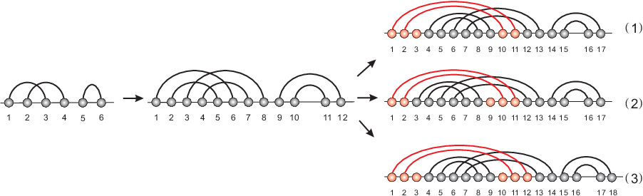
We inflate any shape-arc to a stack of size at least τ\tau and subsequently add additional stacks. The latter are called induced stacks and have to be separated by means of inserting isolated vertices, see Fig. 6. Note that during this first inflation step no intervals of isolated vertices, other than those necessary for separating the nested stacks are inserted.
Refer to caption

Figure 6. The first inflation step a shape (left) is inflated to a 33-noncrossing, 22-canonical structure. First, every arc in the shape is inflated to a stack of size at least two (middle), and then the shape is inflated to a new 33-noncrossing, 22-canonical structure (right) by adding one stack of size two. There are three ways to insert the isolated vertices.

After the first inflation step we proceed inflating further by inserting only additional isolated vertices at the remaining (2​s+1)(2s+1) positions in which such insertions are possible. For each 11-arc at least one such isolated vertex is necessarily inserted, see Fig. 7.

Refer to caption

Figure 7. The second inflation step: the structure (left) obtained in (1) in Fig. 6 is inflated to a new 33-noncrossing, 22-canonical RNA structures (right) by adding isolated vertices (red).

We proceed by expressing the above two inflations in terms of symbolic enumeration. For this purpose we introduce the combinatorial classes ℳ\mathcal{M} (stems), 𝒦τ\mathcal{K}^{\tau} (stacks), 𝒩τ\mathcal{N}^{\tau} (induced stacks), ℒ\mathcal{L} (isolated vertices), ℛ\mathcal{R} (arcs) and 𝒵\mathcal{Z} (vertices), where 𝐙⁡(z)=z{\bf Z}(z)=z and 𝐑⁡(z)=z2{\bf R}(z)=z^{2}. Let μ1\mu_{1}, μ2\mu_{2} and μ3\mu_{3} be the labels for hairpin-loops, interior-loops and bulges, respectively. Then

(3.14) 𝒯γ\displaystyle\mathcal{T}_{\gamma} =\displaystyle= (ℳ)s×ℒ2​s+1−m×([𝒵×ℒ]μ1)m,\displaystyle\left(\mathcal{M}\right)^{s}\times\mathcal{L}^{2s+1-m}\times\left([\mathcal{Z}\times\mathcal{L}]_{\mu_{1}}\right)^{m},
(3.15) ℳ\displaystyle\mathcal{M} =\displaystyle= 𝒦τ×Seq​(𝒩τ),\displaystyle\mathcal{K}^{\tau}\times\textsc{Seq}\left(\mathcal{N}^{\tau}\right),
(3.16) 𝒩τ\displaystyle\mathcal{N}^{\tau} =\displaystyle= 𝒦τ×([𝒵×ℒ]μ3+[𝒵×ℒ]μ3+[(𝒵×ℒ)2]μ2),\displaystyle\mathcal{K}^{\tau}\times\left([\mathcal{Z}\times\mathcal{L}]_{\mu_{3}}+[\mathcal{Z}\times\mathcal{L}]_{\mu_{3}}+[\left(\mathcal{Z}\times\mathcal{L}\right)^{2}]_{\mu_{2}}\right),
(3.17) 𝒦τ\displaystyle\mathcal{K}^{\tau} =\displaystyle= ℛτ×Seq​(ℛ),\displaystyle\mathcal{R}^{\tau}\times\textsc{Seq}\left(\mathcal{R}\right),
(3.18) ℒ\displaystyle\mathcal{L} =\displaystyle= Seq​(𝒵).\displaystyle\textsc{Seq}\left(\mathcal{Z}\right).

and consequently, translating the above relations into generating functions the generating function 𝐓γ​(z,u1,u2,u3){\bf T}_{\gamma}(z,u_{1},u_{2},u_{3}) is given by

(z2​τ1−z21−z2​τ1−z2​(2​u3​z1−z+u2​(z1−z)2))s​(11−z)2​s+1−m​(u1​z1−z)m=(1−z)−1​(z2​τ(1−z2)​(1−z)2−(2​u3​z​(1−z)+u2​z2)​z2​τ)s​(u1​z)m,\begin{split}\left(\frac{\frac{z^{2\tau}}{1-z^{2}}}{1-\frac{z^{2\tau}}{1-z^{2}}\left(2\frac{u_{3}\,z}{1-z}+u_{2}\left(\frac{z}{1-z}\right)^{2}\right)}\right)^{s}\left(\frac{1}{1-z}\right)^{2s+1-m}\left(\frac{u_{1}\,z}{1-z}\right)^{m}\\ =(1-z)^{-1}\left(\frac{z^{2\tau}}{(1-z^{2})(1-z)^{2}-(2u_{3}\,z\,(1-z)+u_{2}\,z^{2})z^{2\tau}}\right)^{s}(u_{1}\,z)^{m},\end{split}

where the indeterminants uiu_{i} (i=1,2,3i=1,2,3) correspond to the labels μi\mu_{i}, i.e. the occurrences of hairpin-loops, interior-loops and bulges. Accordingly, for any two shapes γ1,γ2∈ℐk​(m)\gamma_{1},\gamma_{2}\in{\mathcal{I}}_{k}(m) having ss arcs, we have

(3.19) 𝐓γ1​(z,u1,u2,u3)=𝐓γ2​(z,u1,u2,u3).{\bf T}_{\gamma_{1}}(z,u_{1},u_{2},u_{3})={\bf T}_{\gamma_{2}}(z,u_{1},u_{2},u_{3}).

We set

(3.20) η⁡(u2,u3)=z2​τ(1−z2)​(1−z)2−(2​u3​z​(1−z)+u2​z2)​z2​τ.\eta(u_{2},u_{3})=\frac{z^{2\tau}}{(1-z^{2})(1-z)^{2}-(2u_{3}\,z\,(1-z)+u_{2}\,z^{2})z^{2\tau}}.

and accordingly derive

𝐇k,τ​(z,u1)\displaystyle{\bf H}_{k,\tau}(z,u_{1}) =\displaystyle= ∑m≥0∑γ∈ℐk​(m)𝐓γ​(z,u1,1,1)=∑s≥0∑m=0sik​(s,m)​𝐓γ​(z,u1,1,1),\displaystyle\sum_{m\geq 0}\sum_{\gamma\in\,{\mathcal{I}}_{k}(m)}{\bf T}_{\gamma}(z,u_{1},1,1)=\sum_{s\geq 0}\sum_{m=0}^{s}i_{k}(s,m){\bf T}_{\gamma}(z,u_{1},1,1),
𝐈k,τ​(z,u2)\displaystyle{\bf I}_{k,\tau}(z,u_{2}) =\displaystyle= ∑m≥0∑γ∈ℐk​(m)𝐓γ​(z,1,u2,1)=∑s≥0∑m=0sik​(s,m)​𝐓γ​(z,1,u2,1),\displaystyle\sum_{m\geq 0}\sum_{\gamma\in\,{\mathcal{I}}_{k}(m)}{\bf T}_{\gamma}(z,1,u_{2},1)=\sum_{s\geq 0}\sum_{m=0}^{s}i_{k}(s,m){\bf T}_{\gamma}(z,1,u_{2},1),
𝐁k,τ​(z,u3)\displaystyle{\bf B}_{k,\tau}(z,u_{3}) =\displaystyle= ∑m≥0∑γ∈ℐk​(m)𝐓γ​(z,1,1,u3)=∑s≥0∑m=0sik​(s,m)​𝐓γ​(z,1,1,u3).\displaystyle\sum_{m\geq 0}\sum_{\gamma\in\,{\mathcal{I}}_{k}(m)}{\bf T}_{\gamma}(z,1,1,u_{3})=\sum_{s\geq 0}\sum_{m=0}^{s}i_{k}(s,m){\bf T}_{\gamma}(z,1,1,u_{3}).

It now remains to observe

∑s≥0∑m=0sik​(s,m)​xs​ym=1+x1+2​x−x​y​𝐅k​(x⁡(1+x)(1+2​x−x​y)2).\sum_{s\geq 0}\,\sum_{m=0}^{s}\,i_{k}(s,m)\,x^{s}\,y^{m}=\frac{1+x}{1+2x-xy}{\bf F}_{k}\left(\frac{x(1+x)}{(1+2x-xy)^{2}}\right).

and to subsequently substitute x=η⁡(1,1)x=\eta(1,1) and y=u1​zy=u_{1}\,z for deriving 𝐇k,τ​(z,u1){\bf H}_{k,\tau}(z,u_{1}). Substituting x=η⁡(u2,1)x=\eta(u_{2},1) and y=zy=z in we obtain 𝐈k,τ​(z,u2){\bf I}_{k,\tau}(z,u_{2}) and finally x=η⁡(1,u3)x=\eta(1,u_{3}) and y=zy=z produce the expression for 𝐁k,τ​(z,u3){\bf B}_{k,\tau}(z,u_{3}), whence the theorem. ∎

4. The central limit theorem

For fixed kk-noncrossing, τ\tau-canonical structure, SS, let ℍn,k,τ​(S)\mathbb{H}_{n,k,\tau}(S), 𝕀n,k,τ​(S)\mathbb{I}_{n,k,\tau}(S) and 𝔹n,k,τ​(S)\mathbb{B}_{n,k,\tau}(S) denote the number of hairpin-loops, interior-loops and bulges in SS. Then we have the r.v.s

  • •

    ℍn,k,τ\mathbb{H}_{n,k,\tau}, where ℙ⁡(ℍn,k,τ=t)=hk,τ​(n,t)𝖳k,τ​(n)\mathbb{P}\left(\mathbb{H}_{n,k,\tau}=t\right)=\frac{h_{k,\tau}(n,t)}{{\sf T}_{k,\tau}(n)}

  • •

    𝕀n,k,τ\mathbb{I}_{n,k,\tau}, where ℙ⁡(𝕀n,k,τ=t)=ik,τ​(n,t)𝖳k,τ​(n)\mathbb{P}\left(\mathbb{I}_{n,k,\tau}=t\right)=\frac{i_{k,\tau}(n,t)}{{\sf T}_{k,\tau}(n)}

  • •

    𝔹n,k,τ\mathbb{B}_{n,k,\tau}, where ℙ⁡(𝔹n,k,τ=t)=bk,τ​(n,t)𝖳k,τ​(n).\mathbb{P}\left(\mathbb{B}_{n,k,\tau}=t\right)=\frac{b_{k,\tau}(n,t)}{{\sf T}_{k,\tau}(n)}.

Here hk,τ​(n,t)h_{k,\tau}(n,t), ik,τ​(n,t)i_{k,\tau}(n,t) and bk,τ​(n,t)b_{k,\tau}(n,t) are the numbers of kk-noncrossing, τ\tau-canonical structures of length nn with tt hairpin-loops, interior-loops and bulges. The key for computing the distributions of the above r.v.s are the bivariate generating functions derived in Theorem 3:

(4.1) 𝐇k,τ​(z,u1)\displaystyle{\bf H}_{k,\tau}(z,u_{1}) =\displaystyle= ∑n≥0∑t≥0hk,τ​(n,t)​zn​u1t,\displaystyle\sum_{n\geq 0}\sum_{t\geq 0}h_{k,\tau}(n,t)z^{n}\,u_{1}^{t},
(4.2) 𝐈k,τ​(z,u2)\displaystyle{\bf I}_{k,\tau}(z,u_{2}) =\displaystyle= ∑n≥0∑t≥0ik,τ​(n,t)​zn​u2t,\displaystyle\sum_{n\geq 0}\sum_{t\geq 0}i_{k,\tau}(n,t)z^{n}\,u_{2}^{t},
(4.3) 𝐁k,τ​(z,u3)\displaystyle{\bf B}_{k,\tau}(z,u_{3}) =\displaystyle= ∑n≥0∑t≥0bk,τ​(n,t)​zn​u3t.\displaystyle\sum_{n\geq 0}\sum_{t\geq 0}b_{k,\tau}(n,t)z^{n}\,u_{3}^{t}.

The following proposition is based on Theorem 2 and facilitates the application of Theorem 1.

Proposition 1.

Suppose 2≤k≤72\leq k\leq 7, 1≤τ≤101\leq\tau\leq 10. There exists a unique dominant 𝐇k,τ​(z,es){\bf H}_{k,\tau}(z,e^{s})-singularity, γk,τ​(s)\gamma_{k,\tau}(s), such that for |s|<ϵ|s|<\epsilon, where ϵ>0\epsilon>0:
(1) γk,τ​(s)\gamma_{k,\tau}(s) is analytic,
(2) γk,τ​(s)\gamma_{k,\tau}(s) is the solution of minimal modulus of

(4.4) z2​τ​(1−z)2​(1−z2+z2​τ)((1−z)2​(1−z2+z2​τ)+z2​τ−z2​τ+1​es)2−ρk2=0.\frac{z^{2\tau}(1-z)^{2}(1-z^{2}+z^{2\tau})}{\left((1-z)^{2}(1-z^{2}+z^{2\tau})+z^{2\tau}-z^{2\tau+1}e^{s}\right)^{2}}-\rho_{k}^{2}=0.

and

(4.5) [zn]​𝐇k,τ​(z,es)∼C⁡(s)​n−((k−1)2+k−12)​(1γk,τ​(s))n,[z^{n}]{\bf H}_{k,\tau}(z,e^{s})\sim C(s)\,n^{-((k-1)^{2}+\frac{k-1}{2})}\left(\frac{1}{\gamma_{k,\tau}(s)}\right)^{n},

uniformly in ss in a neighborhood of 00 and continuous C⁡(s)C(s).

Proof.

The first step is to establish the existence and uniqueness of the dominant singularity γk,τ​(s)\gamma_{k,\tau}(s).
We denote

(4.6) ϑ⁡(z,s)\displaystyle\vartheta(z,s) =\displaystyle= (1−z)2​(1−z2+z2​τ)+z2​τ−z2​τ+1​es,\displaystyle(1-z)^{2}(1-z^{2}+z^{2\tau})+z^{2\tau}-z^{2\tau+1}e^{s},
(4.7) ψτ​(z,s)\displaystyle\psi_{\tau}(z,s) =\displaystyle= z2​τ​(1−z)2​(1−z2+z2​τ)​ϑ​(z,s)−2,\displaystyle z^{2\tau}(1-z)^{2}(1-z^{2}+z^{2\tau})\vartheta(z,s)^{-2},
(4.8) ωτ​(z,s)\displaystyle\omega_{\tau}(z,s) =\displaystyle= (1−z)​(1−z2+z2​τ)​ϑ​(z,s)−1,\displaystyle(1-z)(1-z^{2}+z^{2\tau})\vartheta(z,s)^{-1},

and consider the equations

(4.9) ∀ 2≤i≤k;Fi,τ​(z,s)=ψτ​(z,s)−ρi2,\forall\,2\leq i\leq k;\qquad F_{i,\tau}(z,s)=\psi_{\tau}(z,s)-\rho_{i}^{2},

where ρi=1/(2​i−2)\rho_{i}=1/(2i-2). Theorem 3 and Table 1 imply that the singularities of 𝐇k,τ​(z,es){\bf H}_{k,\tau}(z,e^{s}) are are contained in the set of roots of

(4.10) Fi,τ​(z,s)=0andϑ⁡(z,s)=0F_{i,\tau}(z,s)=0\quad\text{and}\quad\vartheta(z,s)=0

where i≤ki\leq k. Let ri,τr_{i,\tau} denote the solution of minimal modulus of

(4.11) Fi,τ​(z,0)=ψτ​(z,0)−ρi2=0.F_{i,\tau}(z,0)=\psi_{\tau}(z,0)-\rho_{i}^{2}=0.

We next verify that, for sufficiently small ϵi>0\epsilon_{i}>0, |z−ri,τ|<ϵi|z-r_{i,\tau}|<\epsilon_{i}, |s|<ϵi|s|<\epsilon_{i}, the following assertions hold

  • •

    ∂∂z​Fi,τ​(ri,τ,0)≠0\frac{\partial}{\partial z}F_{i,\tau}(r_{i,\tau},0)\neq 0

  • •

    ∂∂z​Fi,τ​(z,s)\frac{\partial}{\partial z}F_{i,\tau}(z,s) and ∂∂s​Fi,τ​(z,s)\frac{\partial}{\partial s}F_{i,\tau}(z,s) are continuous.

The analytic implicit function theorem, guarantees the existence of a unique analytic function γi,τ​(s)\gamma_{i,\tau}(s) such that, for |s|<ϵi|s|<\epsilon_{i},

(4.12) Fi,τ​(γi,τ​(s),s)=0 and γi,τ​(0)=ri,τ.F_{i,\tau}(\gamma_{i,\tau}(s),s)=0\quad\text{ and }\quad\gamma_{i,\tau}(0)=r_{i,\tau}.

Analogously, we obtain the unique analytic function δ⁡(s)\delta(s) satisfying ϑ⁡(z,s)=0\vartheta(z,s)=0 and where δ⁡(0)\delta(0) is the minimal solution of ϑ⁡(z,0)=0\vartheta(z,0)=0 for |s|<ϵδ|s|<\epsilon_{\delta}, for some ϵδ>0\epsilon_{\delta}>0. We next verify that the unique dominant singularity of 𝐇k,τ​(z,1){\bf H}_{k,\tau}(z,1) is the minimal positive solution rk,τr_{k,\tau} of Fk,τ​(z,0)=0F_{k,\tau}(z,0)=0 and subsequently using an continuity argument. Therefore, for sufficiently small ϵ\epsilon where ϵ<ϵi\epsilon<\epsilon_{i} and ϵ<ϵδ\epsilon<\epsilon_{\delta}, |s|<ϵ|s|<\epsilon, the module of γi,τ​(s)\gamma_{i,\tau}(s), i<ki<k and δ⁡(s)\delta(s) are all strictly larger than the modulus of γk,τ​(s)\gamma_{k,\tau}(s). Consequently, γk,τ​(s)\gamma_{k,\tau}(s) is the unique dominant singularity of 𝐇k,τ​(z,es){\bf H}_{k,\tau}(z,e^{s}).
Claim. There exists some continuous C⁡(s)C(s) such that, uniformly in ss, for ss in a neighborhood of 00

[zn]​𝐇k,τ​(z,es)∼C⁡(s)​n−((k−1)2+k−12)​(1γk,τ​(s))n.[z^{n}]{\bf H}_{k,\tau}(z,e^{s})\sim C(s)\,n^{-((k-1)^{2}+\frac{k-1}{2})}\left(\frac{1}{\gamma_{k,\tau}(s)}\right)^{n}.

To prove the Claim, let rr be some positive real number such that rk,τ<r<δ⁡(0)r_{k,\tau}<r<\delta(0). For sufficiently small ϵ>0\epsilon>0 and |s|<ϵ|s|<\epsilon,

|γk,τ​(s)|≤rand|δ⁡(s)|>r.|\gamma_{k,\tau}(s)|\leq r\quad\text{and}\quad|\delta(s)|>r.

Then ψτ​(z,s)\psi_{\tau}(z,s) and ωτ​(z,s)\omega_{\tau}(z,s) are all analytic in 𝒟={(z,s)||z|≤r,|s|<ϵ}\mathcal{D}=\{(z,s)||z|\leq r,|s|<\epsilon\} and ψτ​(0,s)=0\psi_{\tau}(0,s)=0. Since γk,τ​(s)\gamma_{k,\tau}(s) is the unique dominant singularity of

𝐇k,τ​(z,es)=ωτ​(z,s)​𝐅k​(ψτ​(z,s)),{\bf H}_{k,\tau}(z,e^{s})=\omega_{\tau}(z,s)\,{\bf F}_{k}(\psi_{\tau}(z,s)),

satisfying

(4.13) ψτ​(γk,τ​(s),s)=ρk2and|γk,τ​(s)|≤r,\psi_{\tau}(\gamma_{k,\tau}(s),s)=\rho_{k}^{2}\quad\text{and}\quad|\gamma_{k,\tau}(s)|\leq r,

for |s|<ϵ|s|<\epsilon. For sufficiently small ϵ>0\epsilon>0, ∂∂z​Fk,τ​(z,s)\frac{\partial}{\partial z}F_{k,\tau}(z,s) is continuous and ∂∂z​Fk,τ​(rk,τ,0)≠0\frac{\partial}{\partial z}F_{k,\tau}(r_{k,\tau},0)\neq 0. Thus there exists some ϵ>0\epsilon>0, such that for |s|<ϵ|s|<\epsilon, ∂∂z​Fk,τ​(γk,τ​(s),s)≠0\frac{\partial}{\partial z}F_{k,\tau}(\gamma_{k,\tau}(s),s)\neq 0. According to Theorem 2, we therefore derive

(4.14) [zn]​𝐇k,τ​(z,es)∼C⁡(s)​n−((k−1)2+k−12)​(1γk,τ​(s))n,[z^{n}]{\bf H}_{k,\tau}(z,e^{s})\sim C(s)\,n^{-((k-1)^{2}+\frac{k-1}{2})}\left(\frac{1}{\gamma_{k,\tau}(s)}\right)^{n},

uniformly in ss in a neighborhood of 00 and continuous C⁡(s)C(s). ∎

After establishing the analogues of Proposition 1 for 𝐈k,τ​(z,u)\mathbf{I}_{k,\tau}(z,u) and 𝐁k,τ​(z,u)\mathbf{B}_{k,\tau}(z,u), see the Supplemental Materials, Theorem 1 implies the following central limit theorem for the distributions of hairpin-loops, interior-loops and bulges in kk-noncrossing structures.

Theorem 4.

Let k,τ∈ℕk,\tau\in\mathbb{N}, 2≤k≤72\leq k\leq 7, 1≤τ≤101\leq\tau\leq 10 and suppose the random variable 𝕏\mathbb{X} denotes either ℍn,k,τ\mathbb{H}_{n,k,\tau}, 𝕀n,k,τ\mathbb{I}_{n,k,\tau} or 𝔹n,k,τ\mathbb{B}_{n,k,\tau}. Then there exists a pair

(μk,τ,𝕏,σk,τ,𝕏2)(\mu_{k,\tau,\mathbb{X}},\sigma_{k,\tau,\mathbb{X}}^{2})

such that the normalized random variable 𝕏∗\mathbb{X}^{*} has asymptotically normal distribution with parameter (0,1)(0,1), where μk,τ,𝕏\mu_{k,\tau,\mathbb{X}} and σk,τ,𝕏2\sigma_{k,\tau,\mathbb{X}}^{2} are given by

(4.15) μk,τ,𝕏=−γk,τ,𝕏′​(0)γk,τ,𝕏​(0),σk,τ,𝕏2=(γk,τ,𝕏′​(0)γk,τ,𝕏​(0))2−γk,τ,𝕏′′​(0)γk,τ,𝕏​(0),\mu_{k,\tau,\mathbb{X}}=-\frac{\gamma_{k,\tau,\mathbb{X}}^{\prime}(0)}{\gamma_{k,\tau,\mathbb{X}}(0)},\qquad\sigma_{k,\tau,\mathbb{X}}^{2}=\left(\frac{\gamma_{k,\tau,\mathbb{X}}^{\prime}(0)}{\gamma_{k,\tau,\mathbb{X}}(0)}\right)^{2}-\frac{\gamma_{k,\tau,\mathbb{X}}^{\prime\prime}(0)}{\gamma_{k,\tau,\mathbb{X}}(0)},

where γk,τ,𝕏​(s)\gamma_{k,\tau,\mathbb{X}}(s) represents the unique dominant singularity of 𝐇k,τ​(z,es){\bf H}_{k,\tau}(z,e^{s}), 𝐈k,τ​(z,es){\bf I}_{k,\tau}(z,e^{s}), and 𝐁k,τ​(z,es){\bf B}_{k,\tau}(z,e^{s}), respectively.

In Tables 2, 3 and 4 we present the values of the pairs (μk,τ,𝕏,σk,τ,𝕏2)(\mu_{k,\tau,\mathbb{X}},\sigma_{k,\tau,\mathbb{X}}^{2}).

k=2k=2 k=3k=3 k=4k=4
μk,τ\mu_{k,\tau} σk,τ2\sigma_{k,\tau}^{2} μk,τ\mu_{k,\tau} σk,τ2\sigma_{k,\tau}^{2} μk,τ\mu_{k,\tau} σk,τ2\sigma_{k,\tau}^{2}
τ=1\tau=1 0.105573 0.032260 0.012013 0.011202 0.003715 0.003641
τ=2\tau=2 0.061281 0.018116 0.009845 0.008879 0.003734 0.003602
τ=3\tau=3 0.043900 0.012752 0.007966 0.007060 0.003200 0.003060
τ=4\tau=4 0.034477 0.009896 0.006680 0.005854 0.002757 0.002622
k=5k=5 k=6k=6 k=7k=7
μk,τ\mu_{k,\tau} σk,τ2\sigma_{k,\tau}^{2} μk,τ\mu_{k,\tau} σk,τ2\sigma_{k,\tau}^{2} μk,τ\mu_{k,\tau} σk,τ2\sigma_{k,\tau}^{2}
τ=1\tau=1 0.001626 0.001612 0.000855 0.000852 0.000505 0.000504
τ=2\tau=2 0.001897 0.001864 0.001123 0.001111 0.000731 0.000726
τ=3\tau=3 0.001693 0.001655 0.001035 0.001021 0.000692 0.000686
τ=4\tau=4 0.001486 0.001448 0.000922 0.000907 0.000624 0.000618

Table 2. Hairpin-loops: The central limit theorem for the numbers of hairpin-loops in kk-noncrossing, τ\tau-canonical structures. We list μk,τ\mu_{k,\tau} and σk,τ2\sigma^{2}_{k,\tau} derived from eq. (4.15).
k=2k=2 k=3k=3 k=4k=4
μk,τ\mu_{k,\tau} σk,τ2\sigma_{k,\tau}^{2} μk,τ\mu_{k,\tau} σk,τ2\sigma_{k,\tau}^{2} μk,τ\mu_{k,\tau} σk,τ2\sigma_{k,\tau}^{2}
τ=1\tau=1 0.015403 0.013916 0.001185 0.001176 0.000264 0.000264
τ=2\tau=2 0.012959 0.011395 0.001823 0.001793 0.000603 0.000599
τ=3\tau=3 0.011075 0.009570 0.001878 0.001837 0.000693 0.000688
τ=4\tau=4 0.009682 0.008261 0.001803 0.001755 0.000700 0.000693
k=5k=5 k=6k=6 k=7k=7
μk,τ\mu_{k,\tau} σk,τ2\sigma_{k,\tau}^{2} μk,τ\mu_{k,\tau} σk,τ2\sigma_{k,\tau}^{2} μk,τ\mu_{k,\tau} σk,τ2\sigma_{k,\tau}^{2}
τ=1\tau=1 0.000090 0.000090 0.000039 0.000039 0.000019 0.000019
τ=2\tau=2 0.000275 0.000274 0.000149 0.000149 0.000090 0.000090
τ=3\tau=3 0.000343 0.000341 0.000198 0.000198 0.000126 0.000126
τ=4\tau=4 0.000359 0.000357 0.000214 0.000213 0.000140 0.000140

Table 3. Interior-loops: The central limit theorem for the numbers of interior-loops in kk-noncrossing,τ\tau-canonical structures. We list μk,τ\mu_{k,\tau} and σk,τ2\sigma^{2}_{k,\tau} derived from eq. (4.15).
k=2k=2 k=3k=3 k=4k=4
μk,τ\mu_{k,\tau} σk,τ2\sigma_{k,\tau}^{2} μk,τ\mu_{k,\tau} σk,τ2\sigma_{k,\tau}^{2} μk,τ\mu_{k,\tau} σk,τ2\sigma_{k,\tau}^{2}
τ=1\tau=1 0.049845 0.042310 0.008982 0.008684 0.003094 0.003058
τ=2\tau=2 0.025088 0.021785 0.005789 0.005597 0.002457 0.002422
τ=3\tau=3 0.015859 0.013979 0.003936 0.003814 0.001762 0.001737
τ=4\tau=4 0.011197 0.009980 0.002878 0.002795 0.001318 0.001301
k=5k=5 k=6k=6 k=7k=7
μk,τ\mu_{k,\tau} σk,τ2\sigma_{k,\tau}^{2} μk,τ\mu_{k,\tau} σk,τ2\sigma_{k,\tau}^{2} μk,τ\mu_{k,\tau} σk,τ2\sigma_{k,\tau}^{2}
τ=1\tau=1 0.001422 0.001414 0.000770 0.000767 0.000463 0.000462
τ=2\tau=2 0.001326 0.001316 0.000817 0.000813 0.000547 0.000546
τ=3\tau=3 0.000991 0.000984 0.000632 0.000629 0.000436 0.000435
τ=4\tau=4 0.000755 0.000750 0.000489 0.000486 0.000342 0.000341

Table 4. Bulges: The central limit theorems for the numbers of bulges in kk-noncrossing, τ\tau-canonical structures. We list μk,τ\mu_{k,\tau} and σk,τ2\sigma^{2}_{k,\tau} derived from eq. (4.15).

5. Proof of Theorem 2

Proof of Theorem 2. We consider the composite function 𝐅k​(ψ​(z,s)){\bf F}_{k}(\psi(z,s)). In view of [zn]​f​(z,s)=γn​[zn]​f​(zγ,s)[z^{n}]f(z,s)=\gamma^{n}[z^{n}]f(\frac{z}{\gamma},s) it suffices to analyze the function 𝐅k​(ψ⁡(γ⁡(s)​z,s)){\bf F}_{k}(\psi(\gamma(s)z,s)) and to subsequently rescale in order to obtain the correct exponential factor. For this purpose we set

ψ~​(z,s)=ψ⁡(γ⁡(s)​z,s),\widetilde{\psi}(z,s)=\psi(\gamma(s)z,s),

where ψ⁡(z,s)\psi(z,s) is analytic in a domain 𝒟={(z,s)||z|≤r,|s|<ϵ}\mathcal{D}=\{(z,s)||z|\leq r,|s|<\epsilon\}. Consequently ψ~​(z,s)\widetilde{\psi}(z,s) is analytic in |z|<r~|z|<\widetilde{r} and |s|<ϵ~|s|<\widetilde{\epsilon}, for some 1<r~, 0<ϵ~<ϵ1<\widetilde{r},\,0<\widetilde{\epsilon}<\epsilon, since it’s a composition of two analytic functions in 𝒟\mathcal{D}. Taking its Taylor expansion at z=1z=1,

(5.1) ψ~​(z,s)=∑n≥0ψ~n​(s)​(1−z)n,\widetilde{\psi}(z,s)=\sum_{n\geq 0}\widetilde{\psi}_{n}(s)(1-z)^{n},

where ψ~n​(s)\widetilde{\psi}_{n}(s) is analytic in |s|<ϵ~|s|<\widetilde{\epsilon}. The singular expansion of 𝐅k​(z){\bf F}_{k}(z), 2≤k≤72\leq k\leq 7, for z→ρk2z\rightarrow\rho_{k}^{2}, follows from the ODEs, see eq. (2.2), and is given by

(5.2) 𝐅k​(z)={Pk​(z−ρk2)+ck′​(z−ρk2)((k−1)2+(k−1)/2)−1​log⁡(z−ρk2)​(1+o⁡(1))Pk​(z−ρk2)+ck′​(z−ρk2)((k−1)2+(k−1)/2)−1​(1+o⁡(1)){\bf F}_{k}(z)=\begin{cases}P_{k}(z-\rho_{k}^{2})+c_{k}^{\prime}(z-\rho_{k}^{2})^{((k-1)^{2}+(k-1)/2)-1}\log(z-\rho_{k}^{2})\left(1+o(1)\right)\\ P_{k}(z-\rho_{k}^{2})+c_{k}^{\prime}(z-\rho_{k}^{2})^{((k-1)^{2}+(k-1)/2)-1}\left(1+o(1)\right)\end{cases}

depending on whether kk is odd or even and where Pk​(z)P_{k}(z) are polynomials of degree ≤(k−1)2+(k−1)/2−1\leq(k-1)^{2}+(k-1)/2-1, ck′c_{k}^{\prime} is some constant, and ρk=1/2​(k−1)\rho_{k}=1/2(k-1). By assumption, γ⁡(s)\gamma(s) is the unique analytic solution of ψ⁡(γ⁡(s),s)=ρk2\psi(\gamma(s),s)=\rho_{k}^{2} and by construction 𝐅k​(ψ⁡(γ⁡(s)​z,s))=𝐅k​(ψ~​(z,s)){\bf F}_{k}(\psi(\gamma(s)z,s))={\bf F}_{k}(\widetilde{\psi}(z,s)). In view of eq. (5.1), we have for z→1z\rightarrow 1 the expansion

(5.3) ψ~​(z,s)−ρk2=∑n≥1ψ~n​(s)​(1−z)n=ψ~1​(s)​(1−z)​(1+o⁡(1)),\widetilde{\psi}(z,s)-\rho_{k}^{2}=\sum_{n\geq 1}\widetilde{\psi}_{n}(s)(1-z)^{n}=\widetilde{\psi}_{1}(s)(1-z)(1+o(1)),

that is uniform in ss since ψ~n​(s)\widetilde{\psi}_{n}(s) is analytic for |s|<ϵ~|s|<\widetilde{\epsilon} and ψ~0​(s)=ψ⁡(γ⁡(s),s)=ρk2\widetilde{\psi}_{0}(s)=\psi(\gamma(s),s)=\rho_{k}^{2}. As for the singular expansion of 𝐅k​(ψ~​(z,s)){\bf F}_{k}(\widetilde{\psi}(z,s)) we derive, substituting the eq. (5.3) into the singular expansion of 𝐅k​(z){\bf F}_{k}(z), for z→1z\rightarrow 1,

(5.4) {P~k​(z,s)+ck​(s)​(1−z)((k−1)2+(k−1)/2)−1​log⁡(1−z)​(1+o⁡(1))for k oddP~k​(z,s)+ck​(s)​(1−z)((k−1)2+(k−1)/2)−1​(1+o⁡(1))for k even\begin{cases}\widetilde{P}_{k}(z,s)+c_{k}(s)(1-z)^{((k-1)^{2}+(k-1)/2)-1}\log(1-z)\left(1+o(1)\right)&\text{\rm for $k$ odd}\\ \widetilde{P}_{k}(z,s)+c_{k}(s)(1-z)^{((k-1)^{2}+(k-1)/2)-1}\left(1+o(1)\right)&\text{\rm for $k$ even}\end{cases}

where P~k​(z,s)=Pk​(ψ~​(z,s)−ρk2)\widetilde{P}_{k}(z,s)=P_{k}(\widetilde{\psi}(z,s)-\rho_{k}^{2}) and ck​(s)=ck′​ψ~1​(s)((k−1)2+(k−1)/2)−1c_{k}(s)=c_{k}^{\prime}\widetilde{\psi}_{1}(s)^{((k-1)^{2}+(k-1)/2)-1} and

ψ~1​(s)=∂zψ~​(z,s)|z=1=γ⁡(s)​∂zψ⁡(γ⁡(s),s)≠0for ​|s|<ϵ.\widetilde{\psi}_{1}(s)=\partial_{z}\widetilde{\psi}(z,s)|_{z=1}=\gamma(s)\partial_{z}\psi(\gamma(s),s)\neq 0\quad\text{\rm for }|s|<\epsilon.

Furthermore P~k​(z,s)\widetilde{P}_{k}(z,s) is analytic at |z|≤1|z|\leq 1, whence [zn]​P~k​(z,s)[z^{n}]\widetilde{P}_{k}(z,s) is exponentially small compared to 11. Therefore we arrive at

(5.5) [zn]​𝐅k​(ψ~​(z,s))∼{[zn]​ck​(s)​(1−z)((k−1)2+(k−1)/2)−1​log⁡(1−z)​(1+o⁡(1))[zn]​ck​(s)​(1−z)((k−1)2+(k−1)/2)−1​(1+o⁡(1))[z^{n}]{\bf F}_{k}(\widetilde{\psi}(z,s))\sim\begin{cases}[z^{n}]c_{k}(s)(1-z)^{((k-1)^{2}+(k-1)/2)-1}\log(1-z)\left(1+o(1)\right)\\ [z^{n}]c_{k}(s)(1-z)^{((k-1)^{2}+(k-1)/2)-1}\left(1+o(1)\right)\end{cases}

depending on kk being odd or even and uniformly in |s|<ϵ~|s|<\widetilde{\epsilon}. We observe that ck​(s)c_{k}(s) is analytic in |s|<ϵ~|s|<\widetilde{\epsilon}. Note that a dependency in the parameter ss is only given in the coefficients ck​(s)c_{k}(s), that are analytic in ss. Standard transfer theorems [3] imply that

(5.6) [zn]𝐅k(ψ~(z,s))∼A(s)n−((k−1)2+(k−1)/2)for some A⁡(s)∈ℂ,[z^{n}]{\bf F}_{k}(\widetilde{\psi}(z,s))\sim A(s)\,n^{-((k-1)^{2}+(k-1)/2)}\quad\text{\rm for some $A(s)\in\mathbb{C}$},

uniformly in ss contained in a small neighborhood of 00. Finally, as mention in the beginning of the proof, we use the scaling property of Taylor expansions in order to derive

(5.7) [zn]​𝐅k​(ψ⁡(z,s))=(γ⁡(s))−n​[zn]​𝐅k​(ψ~​(z,s))[z^{n}]{\bf F}_{k}(\psi(z,s))=\left(\gamma(s)\right)^{-n}[z^{n}]{\bf F}_{k}(\widetilde{\psi}(z,s))

and the proof of the Theorem is complete.

Acknowledgments. This work was supported by the 973 Project, the PCSIRT Project of the Ministry of Education, the Ministry of Science and Technology, and the National Science Foundation of China.

References

  • [1] E.A. Bender. Central and local limit theorems applied to asymptotic enumeration. J. Combin. Theory A. 15(1973) 91–111.
  • [2] W.Y.C. Chen, E.Y.P. Deng, R.R.X. Du, R.P. Stanley, C.H. Yan, Crossings and nestings of matchings and partitions, Trans. Amer. Math. Soc. 359(4) (2007) 1555–1575.
  • [3] P. Flajolet, R. Sedgewick, Analytic combinatorics, Cambridge University Press, New York, 2009.
  • [4] D.J. Grabiner, P. Magyar, Random walks in Weyl chambers and the decomposition of tensor powers, J. Algebr. Comb. 2 (1993) 239–260.
  • [5] E.Y. Jin, J. Qin, C.M. Reidys, Combinatorics of RNA structures with pseudoknots, Bull. Math. Biol. 70(1) (2008) 45–67.
  • [6] E.Y. Jin, C.M. Reidys, Combinatorial design of pseudoknot RNA, Adv. Appl. Math. 42 (2009) 135–151.
  • [7] E.Y. Jin, C.M. Reidys, RNA pseudoknots structures with arc-length ≥3\geq 3 and stack-length ≥σ\geq\sigma, Discrete Appl. Math., to appear.
  • [8] E.Y. Jin, C.M. Reidys, R.R. Wang, Asympotic analysis of kk-noncrossing matchings, arXiv:0803.0848, (2008).
  • [9] D. Kleitman, Proportions of irreducible diagrams, Studies in Appl. Math. 49 (1970) 297–299.
  • [10] R. Nussinov, G. Pieczenik, J.R. Griggs, D.J. Kleitman, Algorithms for loop matchings, SIAM J. of Appl. Math. 35 (1978) 68–82.
  • [11] C.M. Reidys, R.R. Wang, Shapes of RNA pseudoknot structures, submitted.
  • [12] R. Stanley, Differentiably finite power series, Europ. J. Combinatorics 1 (1980) 175–188.
  • [13] M.S. Waterman, Combinatorics of RNA hairpins and cloverleafs. Stud. Appl. Math. 60(1979) 91-96.