On the density-potential mapping in time-dependent density-functional theory
Abstract
The key questions of uniqueness and existence in time-dependent density-functional theory are usually formulated only for potentials and densities that are analytic in time. Simple examples, standard in quantum mechanics, lead however to non-analyticities. We reformulate these questions in terms of a non-linear Schrödinger equation with a potential that depends non-locally on the wavefunction.
pacs
PACS: 31.15.ee, 31.15.ec, 71.15.QeI Introduction
The reduced one-particle probability density (henceforth density tout court) in a gas of identical interacting particles in an external confining potential carries a wealth of information. For example, the linear response of the density to a driving field is related to density-density correlations and the excitation spectrum of the system. By continuity, the density evolution sets the total current through an arbitrary open surface across a finite system driven out of equilibrium, giving access to transport properties, or across a closed surface, giving access to transfer processes out of a chosen volume. The density determines the generalized mean forces on macroscopic degrees of freedom, with which the gas interacts, and hence the coupled dynamics of the two subsystems.
In fact, the theorems of time-dependent (TD) density-functional theory (DFT) prove that, given an initial many-body state, the TD density contains in principle the expectations of all observables of the interacting system, evolving under a TD scalar potential. Following (the much older) ground-state DFT [1, 2], TDDFT calculations operate by constructing a fictitious system of non-interacting electrons, evolving under another TD scalar potential, such that the fictitious system reproduces the electron density of the interacting system. TDDFT thus provides access to the properties of the interacting system via the much more tractable corresponding non-interacting problem. In recent years, TDDFT has become a central tool for a range of problems involving departures from the electronic ground state (GS). Most applications are in the linear-response regime, calculating the electronic excitation spectra and response of atoms, molecules, solids, even biomolecules, exposed to external fields [3]. Real-time electron dynamics in strong fields have also been studied, including electron transfer processes and transport, ionization, high-harmonic generation, and coupled non-adiabatic electron-nuclear dynamics [4].
TDDFT is based on two distinct results. The first is that, under a given particle interaction and for a given initial many-body state , there is a 1:1 correspondence between the ensuing evolution of the density and the external potential acting on the system. This is the Runge-Gross theorem (RG) [5]. It implies that the potential and all other properties of the system are functionals of the density and initial state, and practical calculations hope to approximate some of these functionals accurately.
The second result is that for every density , evolving from a given initial state under a given particle interaction and external potential , there exists an external potential that returns the same density, , under another particle interaction (the key case of interest being ), starting from, in general, another initial state (so long as the two initial states share the same and ). This result is van Leeuwen’s -representability theorem (vL) [6], later extended to TD current DFT [7]. It means that, by contrast with GS DFT, there is no doubt about the existence of a KS system, i.e. a set of non-interacting electrons whose TD density matches that of the interacting system. The -representability difficulty is lessened in the TD case because the TD Schrödinger equation (TDSE) is first-order in time, and the dependence on the initial wavefunction takes care of a large part of the difficulties associated with -representability.
The first result has been proven for potentials that are analytic in time about the initial time (henceforth denoted -analytic), i.e. such that is equal to its Taylor series expansion in about the initial time, for a finite time interval. The second assumes -analytic potentials and densities. There are also two extensions of RG in the linear-response regime that go beyond these analyticity requirements. In the first [8], the short-time density response to “small” but arbitrary potentials has been shown to be unique under two assumptions: that the system starts from a stationary state (not necessarily the GS) of the initial Hamiltonian and that the corresponding linear density-response function is -analytic. In the second [9], uniqueness of the linear density response, starting from the electronic GS, was proven for any Laplace-transformable (in time) potential. As most physical potentials have finite Laplace transforms, this represents a significant widening of the class of potentials for which a 1:1 mapping can be established in the linear-response regime, from an initial GS; this includes e.g. potentials turning on as with , , or with positive non-integer. It covers most cases of physical interest, under these conditions.
The TDSE is a coupled partial differential equation, which inextricably links analyticity properties in space and time. Thus potentials and initial wavefunctions that are (or could be) standard examples in textbooks, in which the potential or the initial wavefunction has some non-analytic properties in space, yield densities that are not analytic in time. We demonstrate this with several examples in the last part of this paper. This implies that the assumptions underlying vL are more restrictive than they may first appear.
In this paper we build on the foundational work in Refs. [5, 6] on the problems of uniqueness and existence in TDDFT. Our goal is to extend the fundamental framework laid there, by suggesting a simultaneous formulation of these two problems, which overcomes the requirement that the potential or density be analytic in time. This formulation is close to (but different from) several problems whose solutions have been proven to exist mathematically. We relate the one-to-one mappings to the existence and uniqueness of solutions to a particular type of non-linear TDSE (NLSE). While there has been a considerable amount of work on the NLSE [10], the particular non-linear structure we have here has not been investigated before, to the best of our knowledge. We do not give a general solution to this problem, but discuss the features of the equation in relation to other NLSEs in the literature. As the existence of solutions of the latter do not require -analyticity, this suggests that the reformulation will be a useful tool for exploring the limitations (or extensions) of our knowledge of the domain of the Runge-Gross functional.
In Section II, we carefully introduce our reformulation. We explore some consequences of the reformulation and what is known about solutions to the NLSE that we find. Section III turns to the motivation behind this endeavor, with the aid of simple examples where the density evolution under -analytic potentials is non-analytic in time.
II Alternative Formulation of the Density-Potential Mapping
It is straightforward to see that, for a given initial state for a system of electrons, a given state-evolution, , can be generated by at most one TD scalar potential , as follows from TDSE
| (1) |
as long as the wavefunction is non-vanishing on a dense set of values of its arguments. Here, , and are the many-electron operators for the total kinetic energy, the electron-electron interaction (with corresponding to non-interacting electrons) and , respectively. That no two distinct ’s can generate the same , up to a physically irrelevant purely time-dependent phase, can be shown by assuming otherwise, inserting into TDSE, and finding , a physically irrelevant purely time-dependent constant.
What RG proves is the much stronger statement that not only the states must be different, but also their one-particle densities,
| (2) |
must differ, under the restriction that the potentials considered are analytic around . Here is the number-density operator for the system of electrons with position operators . This restriction means that potentials that switch on at like , with non-integer, or are not covered by the proof. (Note that the first example is infinitely differentiable, with vanishing derivatives at , while higher-order derivatives of the second and third types diverge as ). These potentials are Laplace-transformable in , and in the linear-response regime starting from the GS are covered by the vL extension of RG [9].
Here, we formulate (but do not prove) a 1:1 mapping defined via the existence and uniqueness properties of the solution to a system of coupled equations. Differentiating the continuity equation (, where is the current density) once with respect to gives [6]
| (3) |
where
| (4) |
with the current-density operator [11].
We now choose a given prescribed density, which we denote by , and a given initial many-electron state , such that , . We then ask, does a potential exist, such that the density it generates via Eqs. (1) and (2), from the chosen initial state, is equal to the prescribed density, , and is this potential unique?
Noting the appearance of the time-evolving state in the evaluation of in Eq. (3), we re-phrase the question by asking whether the coupled equations
| (5) | |||
| (6) |
have a unique solution for and , given the inputs and . At a notional level, these coupled equations work as follows. Eq. (5) determines the potential , at every , as an instantaneous functional of the state ; the (fixed-time) equation is of Sturm-Liouville form, for which a unique locally square-integrable solution exists for strictly positive densities, and locally square-integrable right-hand side [12]. The restriction to nodeless densities is in practice a minor one as most densities of -electron systems do not have nodes; but it certainly excludes a small subset of them, and excludes typical TD and excited-state densities of one-electron systems. The restriction to locally square-integrable right-hand sides (meaning that the integral of the square of the right-hand side over a finite region is finite) is generally satisfied for physical wavefunctions [13]. A formal solution to Eq. (5) is discussed in the appendix. Eq. (6) then determines the evolution of the state, under the potential just obtained, through an infinitesimal time-step to the “next” time, and so on. Eqs. (5) and (6) therefore define the density-potential mapping: if a unique solution to Eqs. (5) and (6) exists for a given , then there is a 1:1 mapping between the density and potential. If, further, the density is -representable, it directly follows that the unique solution reproduces this target density, .
Non--representability can arise in two ways. First, if no solution exists to Eqs. (5)-(6) for a particular , then is not -representable. Second, a solution to systems of equations of type (5)-(6) does not necessarily have [14]. If there does exist a unique solution but one that fails to return the chosen target density, , then this target density is not -representable [15].
The coupled equations (5) and (6) can be expressed as evolution equations as follows. By taking one further -derivative of Eq. (5), we obtain the system of first-order, in time, partial differential equations
| (7) |
for the pair . The initial conditions are the initial state and , given by the solution of
| (8) |
A system of first-order ordinary differential equations with fixed initial conditions always has a unique solution (given appropriate continuity conditions on the right [16], such as Lipschitz continuity). But partial differential equations are more complex. While the initial-value problem for many classes of partial differential equations is known to have a unique solution, to our knowledge, there are no results yet for equations of the form (7).
Instead, we consider a reformulation of the coupled equations (5) and (6) as a NLSE with non-local potential term, i.e. the potential at depends on the wavefunction not just at or near but further away too. The solution for is an instantaneous functional of , and as can be seen from Eq. (5), and its dependence on is quadratic. Denoting this solution symbolically by , Eqs. (5) and (6) now reduce to the effective NLSE
| (9) |
The problems of -representability of the chosen density and of the uniqueness of this representability reduce to the problem of the existence and uniqueness of the solution to Eq. (9) (together with the requirement that the solution returns , whose negation implies that the chosen density is not -representable, as discussed earlier). Two specific issues that bear on this problem are the nature of the non-linearity of this equation and the boundary behaviour of .
NLSEs with non-local interaction were investigated by Ginibre and Velo [17], who in particular proved under certain conditions the existence and uniqueness of short-time solutions. However their non-linear term (a) does not include Coulomb interactions, (b) deals only with the version of Eq. (5) for the ordinary Laplacian, and (c) does not involve derivatives of the wavefunction. Much of the recent mathematical work involves non-linearities depending on the wavefunction and a single derivative, whereas in this case the potential depends non-locally on four derivatives of . For point (b), the results of Ref. [17] could be extended to a general uniformly elliptic operator on the left (i.e. one which has eigenvalues bounded below by a positive constant, everywhere in space), but this is not what we have: the density appearing on the left-hand side of Eq. (5) decays at infinity, so the differential operator on the left is not uniformly elliptic (i.e. is not gapped away from zero). This makes it difficult to obtain estimates on the behavior of at infinity needed to reproduce the Picard iteration needed to show existence and uniqueness as in Ref. [17]. Problem (b) is absent in the simplified case of periodic boundary conditions, and smoothing over Coulomb singularities deals with problem (a) (as would be relevant for solid-state calculations using pseudo-potentials with a smoothed-out interaction term). For example, Burq, Gerard, and Tzvetkov [18] prove short-time existence and uniqueness of the NLSE with local potential term on compact manifolds. However, even in this case it is not clear whether the given NLSE has the hoped-for solution, because of the loss of derivatives (point (c) above). Ref. [19] proves well-posedness for a NLSE that loses two or more derivatives, however for Hamiltonians with local interactions only. Part of the motivation for this paper is the hope that the further analysis of this problem in mathematical physics will stimulate future work.
III Examples of non t-analytic densities
The practical motivation behind a formulation that goes beyond the analyticity requirements of the original Runge-Gross and van Leeuwen theorems is that it is not unusual, and certainly not pathological, for temporal non-analyticity to arise. If it were true that under any particle interaction, a -analytic potential always generates a -analytic density, and vice-versa, then the constructs of Refs. [5] and [6] would be sufficient to provide a self-contained (even if somewhat restrictive) framework for TDDFT. However, we now argue, with the aid of several examples, that in general a -analytic potential need not produce a -analytic density. Although the RG 1:1 mapping holds in such cases, the -representability proof of Ref. [6] does not apply, opening up the question of the existence and uniqueness of a corresponding Kohn-Sham system.
III.1 Spatially non-analytic initial states
In the first set of examples, spatial non-analyticity in the initial wavefunction leads to temporal non-analyticity in the density.
III.1.1 “Bump” initial states: smooth but non-analytic
Consider a free particle in 1d with an initial wavefunction that is constant in space within a region, e.g.
| (10) |
Here, is a constant, and and are assumed to be such that is infinitely differentiable in everywhere. By repeated application of TDSE
| (11) |
we see that, for a point in , all -derivatives of vanish at [20]. Thus, the Taylor series in time for at fixed is
| (12) |
At the points considered, this series exists, and converges (with, furthermore, an infinite radius of convergence), but not to the function itself: . The true wavefunction, , evolves in time, since the initial state is not a free-particle eigenstate. In particular, the true solution will have density from the outer regions, and , dispersing into the inner region, . Therefore, is not analytic in time. Similarly, using
| (13) | |||||
for the Taylor series for the density at we obtain ; it exists and converges, but not to : . Thus, the density is not -analytic, even though the potential () is.
The above arguments may be straightforwardly extended to initial states that have compact support but are smooth: there in the region , while outside this region, . Such functions are sometimes referred to as “bump functions”. The true solution disperses, while the time Taylor series of does not. Although formally solving the TDSE, the Taylor series is not a valid solution because it is not uniformly convergent in the non-constant region. Similar observations and a detailed analysis for free propagation of smooth compactly supported initial states can be found in Ref. [21].
The above example is easily extended to any initial “spline” state
| (14) |
where is the th stationary state, with energy , of some static confining potential , and and are arbitrary (but may, if desired, be assumed to be such as to ensure infinite smoothness everywhere). Starting from this initial state, we consider evolution under the potential . By repeated application of TDSE
| (15) |
for we arrive at and , with the conclusion, again, that neither the wavefunction nor the density is -analytic.
III.1.2 Initial states with a cusp
Consider evolving an initial state with a cusp in free space. We can solve this explicitly in 1d, with:
| (16) |
Using the free-particle propagator
| (17) |
and the integral representation
| (18) |
we obtain
| (19) | |||||
Immediately from , the cusp vanishes, and the initial exponential gradually disperses and develops oscillations in the tail (see Fig. 1, and note the diminishing scale on the vertical axis).
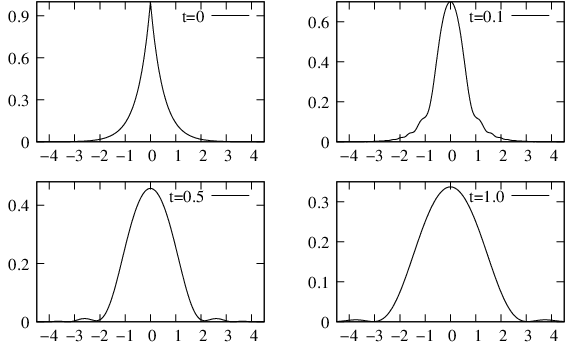
From the Taylor series, away from , we obtain simply
| (20) |
clearly not equal to the true wavefunction (Eq. (19)). Noting that the true solution to TDSE is defined and continuous everywhere, we define such as to make continuous. But then it obeys the TDSE
| (21) |
as opposed to the free-particle TDSE, Eq. (11), obeyed by . Therefore the Taylor series gives a delta-function error in solving the TDSE.
The electron-nuclear Coulomb singularity in 3d gives rise to cusps in stationary states and densities in real systems, i.e. initial states are typically not smooth at the singularity. For example, the GS of the hydrogen atom, , where is the Bohr radius, has analogous mathematical structure to the initial state of Eq. (16). If made to evolve in a potential in which the Coulomb singularity changes (e.g. a nucleus that vanishes, admittedly unphysical), the space-time coupling in the TDSE results in a non-analytic evolving density, in a way that closely follows the above 1d model. We need not however think of the initial state as a GS of any potential: the initial state in Eq. (16) or its 3d analog (or any of the examples given here) can be prepared in many different ways, for example, using particular interferences of free-particle eigenstates. The essential point is that we have a quantum-mechanically allowed initial state, which, when freely-evolved, gives a non--analytic density.
That non--analytic behavior is not a consequence of a change or removal of a singularity in the potential, is shown explicitly in the next example.
III.1.3 Free evolution of the GS of a smooth bounded potential
Consider a free particle in 1d evolving from
| (22) |
where is a (real) constant and is the normalisation constant. This initial wavefunction can be thought of as an example of the earlier bump states, with the interval shrunk to a point. It is the GS of the potential , infinitely differentiable; see Fig. 2 for a plot.

Using Eqs. (17) and (18), we find
| (23) |
and
| (24) |
Neither is -analytic. The non-analyticity in the density takes the form of temporal evolution that picks up infinitely slowly.
To summarize, the examples above illustrate how a non--analytic density may arise from a (trivially) -analytic potential, starting from an initial state that is spatially non-analytic, even though it could be smooth. Indeed Ref. [21] points out that even for the simplest free-particle evolution, starting from an initially smooth state (our examples 1 and 3 are examples thereof), although the Taylor series solution is a formal solution of the TDSE, it is a valid solution only for a very restricted class of initial states, due to non-convergence. Even the time-evolution of the density in a hydrogen atom in an electric field can be shown to be non--analytic [22]. The Runge-Gross theorem applies to all cases, as it is a reformulation of the quantum dynamics of any initial state allowed in quantum mechanics (satisfying appropriate decay at infinity) under a -analytic potential. But in cases where the ensuing evolution is non--analytic, the -representability theorem does not apply.
III.2 Spatially non-analytic potentials
Finally, we consider potentials with the spatial non-analyticity of “bump functions”. We have one particle in 1d, starting from the th stationary state , with energy , of some smooth static confining potential . Now evolve (from ) under the potential
| (25) |
where
| (26) |
Here, is a constant, and and may be chosen such as to give infinite differentiability in everywhere. By applying TDSE repeatedly, for we arrive at and . Since both the wavefunction and the density must evolve, we conclude again that neither of them is -analytic, even though the potential is.
IV Summary and Outlook
TDDFT is an exact reformulation of quantum mechanics in which the density replaces the wavefunction as the basic variable. The density-potential mapping is proven for any initial state evolving under a -analytic potential, such that the density decays appropriately at infinity. The mapping to the KS system is proven for -analytic densities and potentials. However, quite generally, the densities arising from the TDSE are not -analytic, as the simple examples in Sec. III demonstrate. The initial states and potentials considered are certainly within the realm of traditional quantum mechanics, and nothing in the Runge-Gross theorem rules them out from consideration for TDDFT.
The examples suggest that in general a -analytic potential does not give a -analytic density. However, then it is no longer clear that a density, generated by a -analytic potential under one particle interaction, is represented by a -analytic potential under another. This would throw into question the existence and uniqueness of the non-interacting KS system. Therefore, an extension of the TDDFT framework, beyond -analytic potentials and densities, is necessary. The present proposal is that Eqs. (5) and (6) (or their two further formulations in Section II) provide a route to one such extension.
The framing of the fundamental theorems of time-dependent density-functional theories in terms of well-posedness of a type of NLSE first appeared in Ref. [23] where it arises naturally in Tokatly’s Lagrangian formulation of TD current-DFT, known as TD-deformation functional theory. The traditional density-potential mapping question is avoided in TD-deformation functional theory, where instead this issue is hidden in the existence and uniqueness of a NLSE involving the metric tensor defining the co-moving frame. Investigating the relation between the particular NLSE of Ref. [23] and the one in the present paper is an interesting avenue for future work.
It is hoped that these brief considerations will motivate lively work to take these preliminary developments further.
V Acknowledgements
TNT is grateful to EPSRC for support through grant No. EP/C006739/1, and to Queen’s University Belfast for support through a Sabbatical. We also gratefully acknowledge financial support from the National Science Foundation grants CHE-0647913 (NTM) and DMS-060509 (CW), Department of Energy Grant DE-FG02-08ER46496 (KB) and a Research Corporation Cottrell Scholar Award (NTM).
VI Appendix
In this appendix, we explore some interesting properties of the solution to Eq. (5). Specifically, we discuss a reformulation that makes contact with the more standard theory of second-order elliptic operators, namely, operators that are uniformly elliptic at infinity.
We can formally solve Eq. (5) for , with the aid of the transformation
| (27) |
Then Eq. (5) becomes
| (28) |
where
| (29) | |||
| (30) |
We must now solve this equation for . In the following, may be treated as a parameter. The operator has the structure of an ordinary one-particle Hamiltonian. is an eigenfunction of with eigenvalue . Since , is normaliseable (and thus obeys the boundary condition as ). Therefore, is a bound state of . Since the eigenvalue of is zero, for a solution to Eq. (28) for to exist, it is necessary that the right-hand side be orthogonal to ,
| (31) |
Via Eq. (30), this requires to vanish as the surface expands to infinity, which is a condition on the state in the solution of Eqs. (5) (or (28)) and (6). Since the eigenvalue of is zero, furthermore, Eq. (28) defines only up to an arbitrary additive amount of . We choose this amount to be zero. Denoting the eigenfunctions and eigenvalues of by and , respectively, we can then uniquely solve Eq. (28) for :
| (32) |
where
| (33) |
The potential is then obtained from Eq. (27). The given solution for by construction is orthogonal to , and corresponds to a specific choice of the additive spatial constant in [24]. The boundary behaviour at infinity of in Eq. (32), and hence of in Eq. (27), is determined by and by the quantity in Eq. (28).
No difficulty with this solution for arises, if the target density is nodeless. Then too is nodeless, and since it is a bound state of , it must be the GS. Then all other eigenvalues of are positive, in Eq. (33) exists, and the potential in Eq. (27) is defined everywhere.
The situation is more complicated if has nodes. Then, first, may have bound states degenerate with and the requirement of Eq. (31) must be extended to all such states, which constitutes a stronger condition on . (That granted, the formal solution for is then still given by Eq. (32), but with all bound states of , degenerate with , excluded from the definition of in Eq. (33).) Second, both in Eq. (28) and in Eq. (27) may diverge at the nodes of . One would then have to consider the nature of the singularity, and its effect on the propagating state vector.
References
- [1] P. Hohenberg and W. Kohn, Phys. Rev. 136, B 864 (1964).
- [2] W. Kohn and L.J. Sham, Phys. Rev. 140, A 1133 (1965).
- [3] P. Elliott, F. Furche, and K. Burke, Pg 91 in Reviews in Computational Chemistry, Eds. K.B. Lipkowitz and T. R. Cundari (Wiley, Hoboken, NJ 2009 ).
- [4] Time-Dependent Density Functional Theory eds. M.A.L. Marques, F. Nogueira, A.Rubio, K.Burke, C.A. Ullrich, and E.K.U. Gross (Springer, Berlin, 2006).
- [5] E. Runge and E. K. U. Gross, Phys. Rev. Lett. 52, 997 (1984).
- [6] R. van Leeuwen, Phys. Rev. Lett. 82, 3863 (1999).
- [7] G. Vignale, Phys. Rev. B 70, 201102 (2004).
- [8] T. K. Ng and K. S. Singwi, Phys. Rev. Lett. 82, 3863 (1999).
- [9] R. van Leeuwen, Int. J. Mod. Phys. 59, 2627 (1987).
- [10] Semilinear Schrödinger equations, by T. Cazenave (Courant Institute of Mathematical Sciences, 2003).
- [11]
In terms of density matrices, this can be evaluated as
where is the one-body density matrix, is the pair-density (diagonal of the two-body density matrix) and is the electron-electron interaction potential.(34) - [12] See e.g. Theorem 17.2.7 in Hörmander, Analysis of Linear Partial Differential Operators III: Pseudo-Differential Operators (Springer-Verlag, Berlin, Heidelberg, 2007).
- [13] We note that, although not stated there, the same restrictions apply also to the proof in Ref. [6] for the -analytic case. Thorough discussion of the latter may be found in M. Ruggenthaler, M. Penz and D. Bauer, J.Phys.A: Math. Theor. 42, 425207 (2009).
- [14] Theorem 2 Pg 125 in Partial Differential Equations, J. Rauch, (Springer-Verlag, New York, 1991).
- [15] An alternative formulation is to replace the left-hand side of Eq. (5) by . Subtracting Eqs. (3) and (5) then gives , where . The given initial conditions , then guarantee for all . Existence and uniqueness of the solution, for , to this modified formulation is then a necessary and sufficient condition for unique -representability of the chosen target density . However, this formulation makes , as defined by Eq. (5), a more complicated functional of . The distinction between these two formulations is left for future work.
- [16] See e.g. Theory of Ordinary Differential Equations, E. A. Coddington, N. Levinson (New York, McGraw-Hill, 1955) for the Picard-Lindelöf theorem (equivalently, the Cauchy-Lipschitz theorem).
- [17] J. Ginibre and G. Velo, Math Zeitschrifte 170, 109 (1980).
- [18] N. Burq, P. Gerard, and N. Tzvetkov, [Theorem 3.1] in Am. J. Math. 126, 569 (2004).
- [19] C. E. Kenig, G. Ponce, and L. Vega, Invent. Math.134, 489 (1998).
- [20] Here, we have assumed, further, that - and -differentiation may be interchanged, and that this interchangeability survives as .
- [21] B. R. Holstein and A. R. Swift, Am. J. Phys. 40, 829 (1972).
- [22] Z. Yang and K. Burke, unpublished.
- [23] I. Tokatly, Phys. Rev. B. 75, 125105 (2007); Phys. Chem. Chem. Phys. 11, 4621 (2009).
- [24] Since Eq. (28) is of second order, the complementary function in the general solution for contains a second term, in addition to . It too has been eliminated in the solution in Eq. (32).