The Canada-France High- Quasar Survey:
nine new quasars and the luminosity function at redshift 6
Abstract
We present discovery imaging and spectroscopy for nine new quasars found in the Canada-France High- Quasar Survey (CFHQS) bringing the total number of CFHQS quasars to 19. By combining the CFHQS with the more luminous SDSS sample we are able to derive the quasar luminosity function from a sample of 40 quasars at redshifts . Our binned luminosity function shows a slightly lower normalisation and flatter slope than found in previous work. The binned data also suggest a break in the luminosity function at . A double power law maximum likelihood fit to the data is consistent with the binned results. The luminosity function is strongly constrained (1 uncertainty dex) over the range . The best-fit parameters are , break magnitude and bright end slope . However the covariance between and prevents strong constraints being placed on either parameter. For a break magnitude in the range we find at 95% confidence. We calculate the quasar intergalactic ionizing flux and show it is between 20 and 100 times lower than that necessary for reionization. Finally, we use the luminosity function to predict how many higher redshift quasars may be discovered in future near-IR imaging surveys.
Subject headings
cosmology: observations --- quasars: general --- quasars: emission linesI. Introduction
Observations of the most distant quasars provide important information on the state of the universe within the first billion years. They are used to probe the transition from a mostly neutral to mostly ionized intergalactic medium (IGM). They provide the only direct estimates of the metallicities and evolutionary states of massive galaxies. Quasars also probe the very early growth of supermassive black holes in the centers of massive galaxies.
The success of surveys such as the Sloan Digital Sky Survey (SDSS; Fan et al. 2006a; Jiang et al. 2009) and Canada-France High- Quasar Survey (CFHQS; Willott et al. 2009) means that the number of known quasars at is approaching 50. These samples are now large enough to determine the typical properties of quasars over a range of luminosities. One of the most remarkable results is that in most respects, quasars at have properties such as metallicity, emission line strength, hot dust mid-IR luminosity and cool dust far-IR luminosity very similar to lower redshift quasars (Freudling et al. 2003; Iwamuro et al. 2004; Fan et al. 2004; Jiang et al. 2006; Wang et al. 2008).
The number of known quasars is now large enough to allow the luminosity function to be determined. The luminosity function is important since it encodes information about the build-up of supermassive black holes and gives the hard ionizing radiation output of the quasar population. Early work on the quasar luminosity function was based on determining the normalisation, , and bright-end power law slope, , from the SDSS. This was done by direct determination from the known SDSS quasars by Fan et al. (2004) yielding a factor of 30 times lower than at and (95% confidence range of to ). Further constraints came from the lack of gravitational lenses amongst the known SDSS quasars which implied (Fan et al. 2003; Richards et al. 2004). Jiang et al. (2008; 2009) combined the SDSS main sample with the SDSS deep stripe to find a somewhat shallower slope of . However, the binned data shown in Jiang et al. (2009) suggest that there may be a break in the luminosity function at , in which case could be closer to the value determined by Fan et al. (2004).
There have been several small area surveys searching for faint quasars. These are summarized by Shankar & Mathur (2007). Only the key results for surveys at are repeated here. Cool et al. (2006) discovered three quasars at , including one quasar at with , in the AGES survey which covers only 8.5 sq deg. As shown by Jiang et al. (2008), Cool et al. were very fortuitous to discover such a bright quasar at in such a small sky area. The space density of similar luminosity quasars determined by Jiang et al. from the much larger SDSS deep stripe is about six times lower than that of Cool et al.
Mahabal et al. (2005) searched for high-redshift quasars around known SDSS quasars and serendipitously discovered one with magnitude at foreground to a SDSS quasar located at . In total, Mahabal et al. searched 2.5 sq deg. to a depth of . Willott et al. (2005a) searched the first data release (T0001) of the CFHT Legacy Survey Deep and found no quasars to in 3.8 sq. deg. The Mahabal et al. and Willott et al. results reveal that there must be a break in the luminosity function between these low luminosities () and the high luminosity SDSS quasars (). Because low luminosity quasars provide the bulk of ionizing photons from AGN, Willott et al. (2005a) showed that quasars were incapable of reionizing the IGM at , consistent with constraints from the unresolved X-ray background (Djikstra et al. 2004).

In this paper we present the discovery of nine further CFHQS quasars and use a combined CFHQS/SDSS sample to derive the quasar luminosity function. Sec. 2 presents the data on these quasars and notes on each one are given in Sec. 3. Sec. 4 discusses the depth, area and completeness of the parts of the CFHQS and SDSS which are used in this paper to determine the luminosity function. Sec. 5 presents binned and parametric derivations of the quasar luminosity function. Sec. 6 discusses what this new derivation implies for the quasar intergalactic ionizing flux and search strategies for even higher redshift quasars. We present the conclusions in Sec. 7.
All optical and near-IR magnitudes in this paper are on the AB system. Cosmological parameters of , and (Komatsu et al. 2009) are assumed throughout.
| Quasar | RA and DEC (J2000.0) | mag | mag | mag | ||
|---|---|---|---|---|---|---|
| CFHQS J005006+344522 | 00:50:06.67 +34:45:22.6 | |||||
| CFHQS J013603+022605 | 01:36:03.17 +02:26:05.7 | |||||
| CFHQS J142952+544717 | 14:29:52.17 +54:47:17.7 | |||||
| CFHQS J022122-080251 | 02:21:22.71 -08:02:51.5 | |||||
| CFHQS J222901+145709 | 22:29:01.65 +14:57:09.0 | |||||
| CFHQS J210054-171522 | 21:00:54.62 -17:15:22.5 | |||||
| CFHQS J031649-134032 | 03:16:49.87 -13:40:32.3 | |||||
| CFHQS J105928-090620 | 10:59:28.61 -09:06:20.4 | |||||
| CFHQS J224237+033421 | 22:42:37.55 +03:34:21.6 |
Note. — All magnitudes are on the AB system.
| Quasar | Redshift | Date | Resolving | Slit Width | Exp. Time | Seeing | |
|---|---|---|---|---|---|---|---|
| Power | (Arcsec) | (s) | (Arcsec) | ||||
| CFHQS J0050+3445 | 6.25 | 2008 Sep 25 | 4800 | 1.0 | 6250 | 1.3 | |
| CFHQS J0136+0226 | 6.21 | 2009 Aug 02 + 2009 Sep 13 | 1300 | 1.0 | 5400 | 0.9 | |
| CFHQS J1429+5447 | 6.21 | 2009 Mar 31 + 2009 Apr 30 | 1300 | 1.0 | 5400 | 0.9 | |
| CFHQS J0221-0802 | 6.16 | 2008 Oct 24 | 1300 | 1.0 | 5400 | 0.7 | |
| CFHQS J2229+1457 | 6.15 | 2008 Sep 24 | 4800 | 1.0 | 3600 | 0.9 | |
| CFHQS J2100-1715 | 6.09 | 2008 Jul 30 | 1300 | 1.0 | 3600 | 0.7 | |
| CFHQS J0316-1340 | 5.99 | 2009 Aug 02 | 1300 | 1.0 | 3600 | 0.7 | |
| CFHQS J1059-0906 | 5.92 | 2009 Mar 22 | 1300 | 1.0 | 3600 | 0.6 | |
| CFHQS J2242+0334 | 5.88 | 2008 Oct 18 | 1300 | 1.0 | 3600 | 0.5 |
Note. — GMOS spectra have resolving power 1300 and ESI spectra have resolving power 4800. As in Willott et al. (2009), absolute magnitudes () are calculated using the measured -band magnitudes and assuming a template quasar spectrum. Note that this is slightly different to the method used in Willott et al. (2007), which was based on measuring the continuum redward of Ly in the spectrum and assuming a spectral index.
II. New CFHQS quasars
The optical imaging phase of the CFHQS and associated Canada-France Brown Dwarf Survey (CFBDS) is now complete. It draws on the Very Wide (VW), Wide and Deep components of the CFHT Legacy Survey (CFHTLS), the Subaru/XMM-Newton Deep Survey (SXDS) and the Red-sequence Cluster Survey (RCS-2). For some of these surveys, additional imaging was obtained in PI mode to complete the necessary filter coverage. Further details of the observations are given in Willott et al. (2009). Near-IR and spectroscopic follow-up is still ongoing, so this paper does not present the final results of the CFHQS. Sec. IV discusses the complete parts of the CFHQS which are used to determine the quasar luminosity function in this paper.
Quasar candidates were selected using the same color criteria as in Willott et al. (2009). The first cut is at to select very red objects which are a mixture of brown dwarfs and high-redshift quasars. Pointed -band photometry with the ESO New Technology Telescope and Nordic Optical Telescope is then used to separate these two types of object, the dwarfs having redder colors than the quasars. Spectroscopy of candidates was carried out mostly using the GMOS spectrographs at the twin Gemini telescopes. Two quasars (CFHQS J0050+3445 and CFHQS J2229+1457) were observed with the ESI spectrograph at Keck-II. Spectroscopic reductions were performed as detailed in Willott et al. (2007).
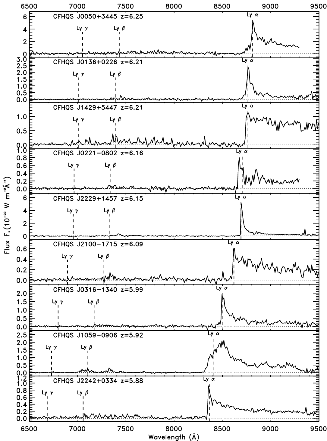
Table 1 gives the positions and photometry for the nine new quasars. Table 2 details the spectroscopic observations. Note in this table and the rest of the paper, quasar names use an abbreviated form. Fig. 1 shows cutout images centred on each quasar and Fig. 2 plots their optical spectra. Larger area finding charts are in the Appendix.
III. Notes on individual quasars
III.1. CFHQS J0050+3445
The redshift of the quasar is based on the narrow peak of Ly emission on top of the broad line. This is consistent with the redshift based on the broad Mg ii emission line (Willott et al. in prep.). This is the second highest redshift in the CFHQS. It is also the second most luminous CFHQS quasar with , which is nearly as luminous as some of the SDSS quasars of Fan et al. (2006b).
This quasar is included in the group of RCS-2/CFHTLS VW quasars, however it is the only one in that group which is not actually located in these survey areas. We carried out band imaging of regions already observed at band with CFHT of the intragroup environment of the Local Group (PI R. Ibata). These observations were necessary to use scheduled time (supposed to be band followup of RCS-2 fields) when the filter broke and was unusable. This field proved not to be ideal for the CFHQS because of several Local Group variable red giant stars which had non-contemporaneous photometry appearing to be quasars, which required repeat photometry to eliminate.
III.2. CFHQS J0136+0226
The spectrum shows a fairly narrow broad Ly line. The redshift of is derived from the peak of the narrow Ly . This is the only quasar in this paper which was not detected in the filter. It has a lower limit on the color of . The color is quite blue for such a high redshift quasar. This is likely because of the high equivalent width Ly emission.
The faint galaxy 3 arcsec north of the quasar (Fig. 1) happened to be located along the spectrograph slit. It has a single emission line at 7468Å which is likely [O ii] at . The low luminosity of this galaxy (at observed frame wavelengths from to band) indicates it has only a moderate mass and at this separation from the quasar will provide negligible gravitational lensing magnification (see e.g. Sec. 4 of Willott et al. 2005b).
III.3. CFHQS J1429+5447
This quasar was discovered in the CFHTLS Wide W3 region. However, it is much brighter than our Wide magnitude limit of and has the second brightest absolute magnitude in this paper. The spectrum shows a strong continuum with only a weak Ly emission line at . This is consistent with the relatively red color of . The spectrum shows a dark Ly absorption trough from with lots of sharp Ly peaks at lower redshift. A more sensitive and higher spectral resolution spectrum is required for a complete analysis.
There is an obvious Mg ii absorption doublet at 9061.5, 9083.8 Å which corresponds to . The apparent broad absorption at 9300 Å is telluric absorption which has not been corrected for (and can be seen for several other quasars in Fig. 2).
III.4. CFHQS J0221-0802
Another quasar from the CFHTLS Wide (W1 field) and the faintest at band in this paper. The Ly emission peaks at with a narrow spike atop an asymmetric broad component. There is also a likely N v line consistent with the Ly redshift. On the other hand, the near-IR spectrum (Willott et al. in prep.) shows the Mg ii line at which we adopt as the systemic redshift for this quasar.
III.5. CFHQS J2229+1457
This is another CFHQS quasar with a strong, very narrow Ly emission line. The best-fit redshift to the peak of the Ly line gives . An unpublished near-IR spectrum shows the Mg ii line to have an identical redshift.
III.6. CFHQS J2100-1715
This quasar has a very similar spectrum to CFHQS J0221-0802 with a narrow Ly peak at (consistent with the unpublished Mg ii line redshift). There is an interesting peak in the Ly forest at which appears too far from the systemic redshift to be within the quasar-ionized near-zone for a quasar of such moderate luminosity. CFHQS J2100-1715 has a rather red color of for its redshift, which may be partly due to the weak Ly line, but also indicates a red spectral slope.
III.7. CFHQS J0316-1340
The spectrum shows a double-peaked Ly emission line. We take the redshift of from the blueward peak. In terms of the spectrum and photometry, there is nothing unusual about this quasar.
III.8. CFHQS J1059-0906
This is one of the few CFHQS quasars to have a very broad Ly line, typical of those in the SDSS main sample. The quasar is fairly bright (), consistent with the idea that line width correlates with luminosity due to the black hole mass. There is no narrow peak to Ly and consequently a large uncertainty on the redshift which is estimated to be based on the full broad Ly profile and expected asymmetry due to hydrogen absorption.
III.9. CFHQS J2242+0334
Yet another quasar with a narrow Ly peak just redward of a sharp cutoff. At and this is the lowest redshift and least luminous quasar from the RCS-2 and CFHTLS Very Wide. It is also the bluest quasar in the CFHQS with . This is not too surprising because the expected colors of quasars have a minimum at (Willott et al. 2009).

IV. CFHQS and SDSS quasar surveys
IV.1. CFHQS
The sample of CFHQS quasars used to derive the luminosity function in this paper contains all the quasars discovered from patches (contiguous sub-regions) which have complete near-IR imaging and spectroscopic follow-up to the full magnitude and color limits. The CFHTLS Wide areas are not included because none of the Wide patches are yet complete. All the quasars from the CFHTLS Deep/SXDS, RCS-2 and CFHTLS VW are located in complete patches. Therefore the CFHQS sample in this paper consists of 12 quasars from the RCS-2 (including CFHQS J0050+3445), 4 quasars from the CFHTLS VW and 1 quasar from the CFHTLS Deep/SXDS. The effective sky areas are 494 sq. deg. for the combination of RCS-2 and CFHTLS VW and 4.47 sq. deg. for the CFHTLS Deep/SXDS. We use the fifth data release (T0005) of the CFHTLS Deep. One of the quasars included in the CFHQS RCS-2 sample was actually discovered by the SDSS (SDSS J2315-0023 at ; Jiang et al. 2008), but as explained in Willott et al. (2009) it was already in our follow-up list before we learned of its discovery. Since this quasar lies within the CFHQS area, it must be included in our sample if we are not to underestimate the number of quasars.
The patches have variable optical imaging depth and therefore careful completeness corrections have to be applied. The method to determine completeness consisted of inserting 1.5 million artificial point sources into our data and determining the fraction recovered by our selection pipeline as a function of magnitude and color. Extensive details of this process are given in the CFBDS paper of Reylé et al. (2009). An example of the resulting completeness as a function of apparent magnitude and color is shown in the left hand panel of Fig. 3.
For the CFHQS quasars, rather than the brown dwarfs in the CFBDS, several further steps are necessary. Galactic extinction affects both the observed color and absolute magnitude, so is corrected for based on the maps of Schlegel et al. (1998). For quasars we need to determine how the color selection cut and completeness affects the redshift completeness. This is particularly important at where the typical quasar color is approximately the same as our color lower limit. We use the 180 cloned SDSS quasars first discussed in Willott et al. (2005a) to determine how the completeness as a function of color translates to completeness as a function of redshift. This process assumes that the spectra of quasars do not evolve significantly from to in accord with most observations (Fan et al. 2004). The only factor that evolves with redshift is the transparency of the IGM to Ly radiation. This is modeled using the empirical fit of Songaila (2004). The proximity of the CFHQS quasars in color-color space to their expected locations (Willott et al. 2009) shows that the cloning process is very effective.
The right hand panel of Fig. 3 shows the completeness as a function of redshift for a typical patch from the RCS-2. Curves are plotted for three different apparent magnitudes. This shows that the completeness does not change much from to . By the time the magnitude limit is reached, the completeness for this RCS-2 patch is about half of its peak value. Part of this decline is due to some regions having 10 limits brighter than and part is due to photometric scatter (the hard cut at misses some objects with intrinsic magnitudes of ). The cut selects quasars at . Most of the lowest redshift CFHQS quasars are expected to be close to the magnitude limit, because the higher magnitude errors increase the number of objects with true colors appearing in the selection box. At quasars move out of the selection box because their colors become like those of late T dwarfs and the absolute magnitude at a fixed magnitude decreases rapidly.
The final step is to convert the CFHQS completeness as functions of redshift and apparent magnitude into functions of redshift and absolute magnitude. This is accomplished by using the 180 cloned lower redshift quasars to mimic the expected variance in the relationship between apparent and absolute magnitude at a fixed redshift. Fig. 4 shows two panels of the completeness as a function of redshift and absolute magnitude for CFHQS. One panel is for all the CFHQS RCS-2/VW patches and one is for the combination of the CFHTLS Deep and SXDS. The locations of quasars in the complete samples used in this paper are also marked. Most quasars were found close to the edge of the selection function in absolute magnitude. The two quasars at in very dark regions of the plot are in regions where the completeness is only . The completeness is so low here because only parts of some patches have high completeness to the magnitude limit of . Effectively, this is equivalent to only a fraction of the full sky area having been surveyed to the full depth.

IV.2. SDSS main sample
The bright end of the quasar luminosity function is best sampled by the SDSS main sample described in Fan et al. (2000; 2001; 2003; 2004; 2006b). The most recent published sample from Fan et al. (2006b) contains 14 quasars at with uniform selection criteria found from a total sky area of sq. deg. The quasars are selected to a magnitude limit of and color cut of . Note that due to differences between the filters used by SDSS and CFHT, the SDSS sample has better completeness at than the CFHQS, despite the apparently higher color cut of the SDSS. This is the reason why the CFHQS sample has a slightly higher median redshift () than the SDSS sample ().
The SDSS main sample completeness as a function of absolute magnitude and redshift was supplied by X. Fan and is that shown in Fig. 7 of Fan et al. (2003). Fan et al. use a slightly different cosmological model to us and therefore their selection function and quasar absolute magnitudes are both converted to our cosmology.
The SDSS main sample completeness as a function of absolute magnitude and redshift is also shown in Fig. 4. The SDSS quasars cluster very strongly to the edge of the selection function indicating a fairly steep bright end slope to the luminosity function. Indeed, Fan et al. (2004) derived a slope of from these data. Two SDSS main quasars are found in regions of very low selection probability (), as was also found for the CFHQS.
IV.3. SDSS deep stripe
A small portion of the SDSS, the deep stripe, has repeated imaging which allows one to search for fainter quasars than can be found in the main sample. Jiang et al. (2008) constructed a sample of six quasars at in a sky area of 260 sq. deg. In a following paper they extended their search to fainter fluxes and found a complete sample of four quasars at in 195 sq. deg (Jiang et al. 2009). These 10 quasars have redshifts between and .
The completeness for the SDSS deep stripe has been determined by Jiang et al. (2008; 2009). In their first paper, quasars were selected using follow-up in either the or filters (the filter is optimum, but was unavailable for some observations). Therefore there are two different selection functions for the and samples (Fig. 5 of Jiang et al. 2008). We combine the and selection functions in proportion to the fraction of quasars discovered with each filter. Note that there are only small differences between these two functions and mostly at the high redshift end where no quasars were detected. The deeper sample of Jiang et al. (2009) covers some of the same area as their brighter sample. We therefore used the brighter sample selection function for 65 sq. deg. and for the remaining 195 sq deg. set the selection function to be the greater of either the bright or faint sample functions. This was necessary because at some locations in the plane, the brighter selection function is actually higher than the fainter selection function.
Fig. 4 shows two panels for the completeness of the two SDSS deep stripe samples. The SDSS deep sample reaches to within half a magnitude of the CFHQS RCS-2/VW sample, but covers less than half the area on the sky. It is apparent that quasars from both the SDSS deep samples do not cluster as strongly to the selection function as either the SDSS main or CFHQS quasars.
As mentioned above, SDSS J2315-0023 from Jiang et al. (2008) was also discovered in CFHQS imaging and is the only quasar to have been identified in the small fraction of overlap in sky area between the CFHQS and SDSS deep stripe. This quasar will be included in both the CFHQS and SDSS deep stripe samples for the purposes of calculating the luminosity function and the sky areas of the samples will be treated as if they are independent. Excluding this duplication, the combined CFHQS and SDSS quasar sample used in this paper consists of 40 quasars at redshifts .
V. z=6 quasar luminosity function
V.1. Binned luminosity function
To help determine the appropriate parametric form of the luminosity function we first carry out a simple binning of the data. As is well known, the main disadvantage of this method is that for small samples with inhomogeneous coverage of parameter space, the choice of bins can make large differences to the results. In addition, binned luminosity functions are difficult to extrapolate beyond well-sampled parts of parameter space.
We use the binned method of Avni & Bahcall (1980) where is the co-moving volume available for a source in a bin with sizes and . Due to the small number of quasars and small range in redshift, we only use one redshift bin. In the following section we will discuss the likely amount of evolution across this bin. The available volume takes into account the selection functions, , described in Sec. IV and can be calculated as
The volume element accounts for the sky area of the survey(s) at this location in space. The luminosity function, , is then calculated as
The absolute magnitude bins were chosen to avoid human-induced bias as much as possible. No attempt was made to get approximately equal numbers of objects in each bin, since this can bias the results for small samples.
Unlike in the work of Jiang et al. (2009) which treated their and samples separately , we combine the two SDSS deep stripe samples of Jiang et al. (2008; 2009) so that the SDSS deep quasars are in bins determined by their rather than their apparent magnitude.

Fig. 5 shows the binned luminosity function derived from the CFHQS and SDSS samples. Data points are plotted at the mean absolute magnitude of objects within the bin. Separate points are plotted for the CFHQS, SDSS main and SDSS deep stripe samples, even though there is some overlap in absolute magnitude of the three samples. Note that due to a different choice of bins sizes, different SDSS main sample size (Jiang et al. included some unpublished quasars) and different cosmological parameters, the SDSS points are not in exactly the same locations as in Jiang et al. (2009).
The dashed lines in Fig. 5 are the two power law fits to the binned luminosity function by Jiang et al. (2009), corrected for our cosmology. The steeper slope line () is a fit to the SDSS main and SDSS deep binned points and the flatter slope () is a fit to the SDSS main and all SDSS deep binned points in Jiang et al. (2009). These power laws from Jiang et al. lie above the SDSS binned points we have calculated. The likely reasons for this difference are because we used different bins and have a different SDSS main sample size. We set the bins to cover absolute magnitude ranges without considering the distribution of data points within each bin. Jiang et al. (2008, 2009) set the edges of their absolute magnitude bins to be equal to the maximum and minimum absolute magnitudes of the objects within the bins (L. Jiang, priv. comm.). For very few objects in the bin this necessarily biases the estimate of the volume available in the bin to low values and hence unreasonably high space densities. This is particularly apparent for the brightest SDSS deep stripe point and faintest SDSS main sample point. A power law fit to our SDSS bins would show a somewhat flatter slope and lower normalisation than either of those found by Jiang et al. However, the discussion above highlights the perils of determining the luminosity function from binned data and we therefore leave any parametric derivation to the following section.
There are three CFHQS binned points on Fig. 5. The faintest point at contains the single quasar from the Deep/SXDS. The other two points contain all the quasars from the RCS-2/VW. The point at contains 12 quasars and has by far the smallest statistical error of any points on the plot. The two RCS-2/VW points lie below the luminosity function defined by the SDSS main and deep stripe binned data. However, these data are all consistent within the size of the 1 error bars, so we do not consider the SDSS and CFHQS data to be in conflict. Considering all the data points together, there appears to be some evidence for a flattening of the luminosity function going from high to low luminosity. The main evidence for a break at is based on the two faintest CFHQS bins. Unfortunately, the small sky area probed by the Deep/SXDS and the single quasar found means that the space density at very low luminosities is not strongly constrained. We will revisit this issue in the following section.
V.2. Parametric luminosity function
To overcome the limitations of the binned method, we also fitted a parametric luminosity function model to the data. As shown by the binned data in Fig. 5 the luminosity function is fit well by a power law at the high luminosity end, with the possibility of a break at low luminosity. In keeping with previous work, we therefore consider the quasar luminosity function at to follow a double power law function:
We include an evolution term because the quasar space density is well known to decline with redshift from a peak at (e.g. Richards et al. 2006). Our sample has only a small redshift range so we do not attempt to fit for the evolution parameter , but adopt the value of which is derived from the evolution from to for the bright end of the luminosity function (Fan et al. 2001). This rate of evolution corresponds to a factor of 2 decrease in space density across our redshift range from to . Hence it is important to include because redshift and absolute magnitude can be correlated in these color- and magnitude-limited samples (e.g. Fig. 4).
This leaves four parameters to be determined:the normalisation , the break magnitude , the bright end slope and the faint end slope . As can be seen in Fig. 5, there are very few quasars in our sample at magnitudes well below the break in the luminosity function. Therefore we have decided to fix the faint end slope to as indicated by AGN surveys at lower redshift (Croom et al. 2004; 2009; Hunt et al. 2004). The remaining three parameters are determined via a maximum likelihood fit (Marshall et al. 1983). The aim is to minimise the function S which equals , where is the likelihood:
where the first term is a sum over each quasar and the second is integrated over the full possible range of redshift and absolute magnitude. Initial starting values of the free parameters were estimated from the binned luminosity function. The parameters were optimised using the amoeba routine (Press et al. 1992).

The best-fit luminosity function parameters are , , . This function is plotted on Fig. 5 as the thick line. It passes through the error bars on each of the binned data points showing good agreement between the maximum likelihood and binned methods. The quasar space density at is a factor of two smaller than that of the fit to binned data of Jiang et al. (2009). This has important consequences for the quasar ionizing photon output at as we shall see later.
Uncertainties on the luminosity function parameters were determined assuming a distribution of () (Lampton, Margon & Bowyer 1976). Due to the fact that the parameters are highly correlated the most useful constraints to consider are those on the joint probability of break absolute magnitude and bright end slope. Note that the faint end slope was always fixed at , so any extra uncertainty due to this is unaccounted for.
Fig. 6 plots the confidence regions for the combination of break absolute magnitude and bright end slope. The parameters are obviously correlated such that bright break magnitudes are consistent with steep bright end slopes. The correlation is easy to understand because a bright break combined with a steep bright end slope would give a similar ratio of bright SDSS to faint CFHQS quasars as a luminosity function with a faint break and flatter bright end slope. This correlation tends to disappear when the break magnitude is fainter than because we have few quasars at such faint levels. The 68.3% confidence region extends off the bottom of this plot, which effectively corresponds to an unbroken power law down to our faintest quasar ().
The reliability of the parameter uncertainties were checked by bootstrap resampling of the data and re-running the maximum likelihood fit on these samples (Press et al. 1992). 100 bootstrap trials were performed. A comparison of the fraction of bootstrap trials within various regions of the confidence contours in Fig. 6 showed very good agreement. 25% of the bootstrap trials gave with in the range to , which effectively means that the power law is unbroken down to our faintest quasar. Although formally allowed by the data, as mentioned above, this would be quite unusual given the double-power law form and break magnitudes observed at lower redshifts. The 100 bootstrap trials are shown in thin grey lines on Fig. 5 to illustrate the range of possible luminosity functions allowed by the data. The space density is very well constrained over the range with the 1 uncertainty being less than 0.1 dex.
In order to try to break the degeneracy between break magnitude and bright end slope, and to assess evolution of the quasar luminosity function, we consider the results from studies at lower redshift. Croom et al. (2009) presented the quasar luminosity function at based on the 2SLAQ and SDSS surveys. They had sufficient spread in luminosity and redshift to be able to determine the luminosity function in narrow () redshift slices. They found evolution in the break magnitude and steep end slope (note that and are swapped in Croom et al. compared to our definition). The evolution in is quite mild with a steepening towards higher redshift. Most of the evolution is in the break magnitude which brightens by 4 magnitudes from to (this is the so-called pure luminosity evolution that characterised early derivations of the evolving quasar luminosity function, e.g. Mathez 1976). The break magnitude and found by Croom et al. (2009) are plotted on Fig. 6 (we converted from to using the relation in Croom et al. and adapted for our cosmology). The parameters at are always located at regions in the plot outside of the 95% confidence region, with the low redshift slope being steeper than that at for a given break magnitude.
Richards et al. (2006) determined the quasar luminosity function up to using the SDSS DR3. At they fit a model with a redshift-dependent bright end slope and fixed break magnitude (due to the fact they did not have any quasars below the break at high redshift). Their fit showed the bright end slope flattening from at to at . This is shown on Fig. 6 by the orange line with points at . Support for the choice of break magnitude adopted by Richards et al. (2006) comes from the luminosity function derived by Siana et al. (2008) using SDSS and SWIRE. In fact, the break magnitude and slope found by Siana et al. (2008) for (pink triangle on Fig. 6) are very close to the minimum best fit at . This would suggest little evolution in these parameters from to , however, there is a considerable range at 95% confidence for .
The studies at lower redshift have shown that at all redshifts in the range , the break magnitude lies between . Therefore we assume that this also holds true at in order to provide tighter constraints on . Under this assumption we find the 95% confidence ranges for to be for and at .
Throughout all the above analysis, the faint end slope was fixed at based on evidence for at lower redshift (Croom et al. 2004; 2009; Hunt et al. 2004). We have checked to see how our results would change if instead we adopted a different value for . We re-ran the maximum likelihood fitting assuming and determined best-fit parameters of , and . Although these best-fit parameters appear substantially different to those for , the two luminosity functions are very similar over the luminosity range covered by the SDSS and CFHQS quasars. The steeper bright end slope and higher break luminosity are shifted along the same direction as the correlation in Fig. 6. The best-fit break at is more luminous than as measured at lower redshifts and as noted above we find it unlikely that the break would be this luminous at . Future large area, deep quasar surveys are necessary to determine the faint end slope.
V.3. Consistency of luminosity function with redshift distributions
These colour-selected quasar samples can only find quasars within a certain redshift range as shown in Figs. 3 and 4. The successful derivation of a luminosity function from these data depends upon accurately determining how the completeness depends upon redshift and luminosity. In order to check the consistency of the observed redshift distributions with the selection function we have used the selection functions and the best-fit luminosity function to generate expected redshift distributions for 3 samples: SDSS main, SDSS deep stripe (combined and ) and CFHQS RCS-2/VW. These expected redshift distributions were then compared to the observed redshift distributions. A Kolmogorov-Smirnov test was applied to determine the probability that the redshift distributions were consistent. The results showed that all samples are consistent with their expected redshift distributions (at probabilities 0.48, 0.78, 0.27, respectively). Jiang et al. (2009) noted that their SDSS deep sample had no quasars at and showed that this lack of high-redshift quasars was not statistically significant. Our findings agree and show that all the samples have redshift distributions as expected from the colour selection criteria.
VI. Applications of the luminosity function
VI.1. The quasar intergalactic ionizing flux at
The constraints placed on the low luminosity end of the quasar luminosity function here are considerably tighter than in previous works (Willott et al. 2005a; Shankar & Mathur 2007; Jiang et al. 2009). Therefore it is useful to consider the ionizing photon output of the quasar population at . We use the 100 bootstrap trial luminosity functions to determine the plausible statistical range of the photon output. Since the luminosity function is not constrained at , we set all the bootstrap models with break magnitudes fainter than this to have a break to at . Note however that we do not include ranges on other important parameters, such as the faint end slope (assumed -1.5 here), the quasar UV spectral slope (assumed that of Telfer et al. 2002) or the photon escape fraction (assumed 100%).
The resulting probability distribution in ionizing photon rate density is shown in Fig. 7. The peak of the distribution is at photons s-1 Mpc-3 and the median is at photons s-1 Mpc-3. The probability distribution is bimodal because the group of bootstrap luminosity functions with have a large number of faint quasars and total emission rate density of photons s-1 Mpc-3. Our results are significantly lower than that previously assumed of photons s-1 Mpc-3 (Meiksin 2005; Bolton & Haehnelt 2007). Because low-luminosity quasars could dominate the ionizing flux, the bootstrap resampling was also run for a steeper faint end slope of and in this case the probability distribution is only shifted 0.1 dex higher than for .

Also, plotted on Fig. 7 is a dashed line to denote the photon rate density required in order to balance recombinations and keep the universe ionized. We follow Meiksin (2005) to calculate this number and assume that the clumpiness factor . It is evident from this plot that the quasar population, even including the possibility of a large number of faint quasars, is insufficient to get even close to the required photon emission rate density. Our estimate of the photon rate density is between 20 and 100 times lower than the required rate. This is consistant with the constraints placed on this rate by the unresolved X-ray background (Djikstra et al. 2004). In comparison, the known galaxy luminosity function at shows that galaxies provide between and photons s-1 Mpc-3 (Ouchi et al. 2009).

VI.2. Search strategies for quasars at even higher redshifts
Now that quasars are known at redshifts , the next challenge is to identify quasars at even higher redshifts. This is particularly important given the possible rapid evolution in the ionization state of the IGM at these redshifts (e.g. Fan et al 2006c). As has been well documented, it is challenging to discover quasars at higher redshifts as the Ly line and continuum move into the near-IR. Several large surveys are now underway or planned aiming to discover quasars at . Given our latest determination of the luminosity function at , we can predict the number of quasars that may be detectable at higher redshifts. The main aim of these predictions is to investigate the optimum observing strategy in a fixed observing time, i.e. wide–shallow vs narrow–deep.
We calculate the density of quasars on the sky as a function of limiting apparent magnitude in three redshift slices (, , ). The calculations are performed for all 100 of the bootstrap resampled luminosity functions. The evolution is assumed to continue as density evolution at the same exponential rate as determined for luminous quasars by Fan et al (2001) from to (i.e. with ). The actual quasar evolution is obviously completely unknown and it is possible that some luminosity-dependence of the evolution occurs over this redshift range. Theoretical models based on Eddington-limited accretion of the quasar population traced back to earlier epochs predict that the black hole accretion rate density is somewhere between 10 and 100 times lower at than (Li et al. 2007; Sijacki et al. 2009). Note that these models are focussed on overdense regions, due to simulation limitations, so may not represent typical regions. However, their evolution compares well with our factor of evolution in space density from to .
Recent deep imaging from WFC3 onboard Hubble Space Telescope and from the ground has enabled the identification of galaxies up to (Ouchi et al. 2009; Bouwens et al. 2009; Oesch et al. 2009). Assuming these galaxies are not mostly low redshift interlopers (see Capak et al. 2009), the evolution in the galaxy luminosity function from to and is not too rapid. Bouwens et al. (2009) and McLure et al. (2009) show the faint end evolution from to is less than a factor of ten. Furthermore, Labbe et al. (2009) show the stellar mass density evolves only by a factor of three between and . Although it is unclear how the evolution of mostly low luminosity galaxies relates to that of luminous quasars, these results are consistent with the evolution for quasars we have adopted.
Fig. 8 shows the 100 bootstrap quasar count predictions in each of the three redshift slices. The expected counts are most strongly constrained for quasars with similar absolute magnitude to the SDSS and CFHQS quasars, corresponding to observed magnitudes 20 to 23. Fontanot et al. (2007a) made similar predictions for the near-IR quasar number counts based on extrapolation of the luminosity functions of Fontanot et al. (2007b) at and Shankar & Mathur (2007) at . They did not show results for the bright end of the luminosity function at apparent magnitudes . At our results are consistent with the predictions based on the evolving model of Fontanot et al. (2007b).
We now consider the specifics of various ongoing and future near-IR sky surveys which might be able to discover high- quasars. All limiting magnitudes are given as AB magnitudes, because experience of the CFHQS shows that this level of photometric accuracy in the bands redward of the Ly line is necessary for reliable colour selection. It should also be noted that we simply consider whether these surveys cover sufficient depth and area at band to be able to detect the quasars. Successful quasar discovery depends upon colour criteria that isolate the quasars from all contaminants such as brown dwarfs. This usually means that data in filters shortward of the Ly break must go 1 to 2 magnitudes deeper than the band data.
The UKIRT Infrared Deep Sky Survey (UKIDSS; Lawrence et al. 2007) began in 2005 and should be completed in a few years. It has several components of which the two we consider here are the Large Area Survey (LAS; 4000 sq. deg. to ) and the Ultra Deep Survey (UDS; 0.77 sq. deg. to ). A primary goal of the LAS is to find quasars (Hewett et al. 2006) and it so far has found two at (Venemans et al. 2007; Mortlock et al. 2009). In Fig. 8, these surveys are plotted alongside the 100 bootstrap predictions such that the location on the plot indicates that one quasar would be found in the survey in that redshift slice. At the LAS falls below the predictions indicating that between 1 and 3 quasars would be expected in this survey at this redshift. The UDS lies right at the upper edge of the predicted quasar counts meaning that it is likely that it will contain quasar at . Note that the UDS forms part of the deep component of the CFHQS and the lone deep CFHQS quasar at actually lies within the UDS. At higher redshifts, the LAS may contain quasar at , but it is very unlikely for the UDS to contain any higher redsift quasars. In conclusion, the wide area component of UKIDSS is much better suited to discovering high- quasars than the deep component.
Set to commence imminently, the ESO VISTA Telescope surveys (Sutherland 2009) are more efficient than UKIDSS due to the use of a larger camera. There are four components of the VISTA surveys that could potentially detect high- quasars. These are VISTA Hemisphere Survey (VHS; 5000 sq. deg. to coincident with the Dark Energy Survey in the optical), VISTA Kilo-Degree Infrared Galaxy Survey (VIKING; 1500 sq. deg. to coincident with VST KIDS in the optical), VISTA Deep Extragalactic Observations Survey (VIDEO; 15 sq. deg. to ) and UltraVISTA (0.73 sq. deg. to in the COSMOS field). As shown on Fig. 8 these surveys should be deep enough at to detect many quasars at and a few at . The most suitable surveys are the wider area surveys of VHS and VIKING, rather than VIDEO and UltraVISTA. This is a consequence of the relatively shallow luminosity function we have found. With a slope of , more quasars can be found in a wide area shallow survey than a narrow area deep survey in a fixed observing time. However, we caution that if the bright end of the luminosity function steepens at high redshift, due for example to the lack of time available for the build-up of the required mass black holes, then this would reverse the situation. Therefore VIKING is probably more likely to yield quasars than VHS. Finally, we note that none of the VISTA surveys are likely to detect quasars.
What about the longer-term future? Several ambitious dark energy projects are being planned such as Euclid and JDEM. These would use some combination of supernovae, baryonic acoustics oscillations and weak lensing to determine the parameters governing the evolution of dark energy. In order to make these measurements it is necessary to make deep surveys of large sky areas in the near-IR and therefore such surveys would also be useful to detect the most distant quasars. Given the early planning stage it is not known yet how much sky area will be covered to what depth. For the purposes of this exercise we use a preliminary Euclid plan which include a wide 20 000 sq. deg. imaging survey to for weak lensing and a deep imaging survey of 30 sq. deg. to for supernovae. The green circles on Fig. 8 show that the wide survey is much more effective at detecting distant quasars due to the flatter faint end slope (note this is not strictly a fair comparison because to these depths and areas in a single filter, the wide survey requires 17 times as long as the deep survey). The wide survey would be able to detect quasars at , at and at . As before, we caution that sufficiently deep data at filters below the Ly break are necessary to provide accurate colours, so this is an upper limit to the number of quasars that might be discoverable. We do not consider even deeper surveys over small sky areas with JWST, because the luminosity function is not well constrained for such low luminosity quasars.
VII. Conclusions
We have presented discovery data for nine new quasars in the CFHQS, bringing the total number so far to 19. The CFHQS is nearing completion and ongoing follow-up may find a few more CFHQS quasars. Further observations of CFHQS quasars are being pursued to understand reionization, black hole mass growth and host galaxy evolution.
The CFHQS and SDSS surveys were combined to derive the quasar luminosity function from a sample of 40 quasars. The normalisation of the luminosity function is found to be % lower than that determined previously using binned data (Jiang et al. 2008; 2009). The luminosity function is well constrained down to but has a large uncertainty at where our faintest quasar is. Future larger sky area, deep surveys, such as VISTA VIDEO, are necessary to constrain this part of the quasar luminosity function. We are also working on measuring black hole masses for quasars. In a future paper we will combine our knowledge of the luminosity function and black hole mass distribution to consider the growth of black holes at this early epoch.
We have calculated the quasar ionizing flux based on possible realizations of the quasar luminosity function and found that the ionizing photon output of quasars is between 20 and 100 times lower than the rate required to keep the universe ionized. Predictions have been made for the number of quasars that might be found by current and future surveys. Whilst UKIDSS may find a few quasars at , the VISTA surveys should find many more and even some up to . Obtaining large samples of quasars and pushing to even higher redshifts will require even more ambitious projects such as Euclid or JDEM.
References
- [1] Avni Y., & Bahcall J.N., 1980, ApJ, 235, 694
- [2] Bolton, J. S., & Haehnelt, M. G. 2007, MNRAS, 382, 325
- [3] Bouwens, R. J., et al. 2009, ApJL, submitted, arXiv:0909.1803
- [4] Capak, P., et al. 2009, ApJ, submitted, arXiv:0910.0444
- [5] Cool, R. J., et al. 2006, AJ, 132, 823
- [6] Croom, S. M., Smith, R. J., Boyle, B. J., Shanks, T., Miller, L., Outram, P. J., & Loaring, N. S. 2004, MNRAS, 349, 1397
- [7] Croom, S. M., et al. 2009, MNRAS, 399, 1755
- [8] Dijkstra, M., Haiman, Z., & Loeb, A. 2004, ApJ, 613, 646
- [9] Fan, X., et al. 2000, AJ, 120, 1167
- [10] Fan, X., et al. 2001, AJ, 122, 2833
- [11] Fan, X., et al. 2003, AJ, 125, 1649
- [12] Fan, X., et al. 2004, AJ, 128, 515
- [13] Fan, X., et al. 2006a, AJ, 132, 117
- [14] Fan, X., et al. 2006b, AJ, 131, 1203
- [15] Fan, X., Carilli, C. L., & Keating, B. 2006c, ARA&A, 44, 415
- [16] Fontanot, F., Somerville, R. S., & Jester S. 2007a, arXiv0711.1440
- [17] Fontanot, F., Cristiani, S., Monaco, P., Nonino, M., Vanzella, E., Brandt, W. N., Grazian, A., & Mao, J. 2007b, A&A, 461, 39
- [18] Freudling, W., Corbin, M. R., & Korista, K. T. 2003, ApJ, 587, L67
- [19] Hewett, P. C., Warren, S. J., Leggett, S. K., & Hodgkin, S. T. 2006, MNRAS, 367, 454
- [20] Hunt, M. P., Steidel, C. S., Adelberger, K. L., & Shapley, A. E. 2004, ApJ, 605, 625
- [21] Iwamuro, F., Kimura, M., Eto, S., Maihara, T., Motohara, K., Yoshii, Y., & Doi, M. 2004, ApJ, 614, 69
- [22] Jiang, L., et al. 2006, AJ, 132, 2127
- [23] Jiang, L., et al. 2007, AJ, 134, 1150
- [24] Jiang, L., et al. 2008, AJ, 135, 1057
- [25] Jiang, L., et al. 2009, AJ, 138, 305
- [26] Komatsu, E., et al., 2009, ApJS, 180, 330
- [27] Labbe, I., et al. 2009, ApJL, submitted, arXiv:0910.0838
- [28] Lampton, M., Margon, B., & Bowyer, S. 1976, ApJ, 208, 177
- [29] Lawrence, et al. 2007, MNRAS, 379, 1599
- [30] Li, Y., et al. 2007, ApJ, 665, 187
- [31] Marshall, H. L., Tananbaum, H., Avni, Y., & Zamorani, G. 1983, ApJ, 269, 35
- [32] Mathez, G., 1976, A&A, 53, 15
- [33] McLure, R. J., Dunlop, J. S., Cirasuolo, M., Koekemoer, A. M., Sabbi, E., Stark, D. P., Targett, T. A., & Ellis, R. S. 2009, MNRAS, submitted, arXiv:0909.2437
- [34] Meiksin, A. 2005, MNRAS, 356, 596
- [35] Mortlock, D., et al. 2009, A&A, 505, 97
- [36] Oesch, P. A., et al. 2009, ApJL, submitted, arXiv:0909.1806
- [37] Ouchi, M., et al. 2009, ApJ, 706, 1136
- [38] Press, W. H., Teukolsky, S. A., Vetterling, W. T., & Flannery, B. P. 1992, Numerical Recipes in C: The Art of Scientific Computing (Cambridge: Cambridge Univ. Press)
- [39] Reylé, C. et al. 2009, A&A, submitted
- [40] Richards, G. T., et al. 2004, AJ, 127, 1305
- [41] Richards, G. T., et al. 2006, AJ, 131, 2766
- [42] Schlegel, D. J., Finkbeiner, D. P., & Davis, M., 1998, ApJ, 500, 525
- [43] Shankar, F. & Mathur, S. 2007, ApJ, 660, 1051
- [44] Siana, B,. et al. 2008, ApJ, 675, 49
- [45] Sijacki, D., Springel, V., & Haehnelt, M. G. 2009, MNRAS, 400, 100
- [46] Songaila, A. 2004, AJ, 127, 2598
- [47] Sutherland, W. Science with the VLT in the ELT Era, Astrophysics and Space Science Proceedings, Volume . ISBN 978-1-4020-9189-6. Springer Netherlands, 2009, p. 171
- [48] Telfer, R. C., Zheng, W., Kriss, G. A., & Davidsen, A. F. 2002, ApJ, 565, 773
- [49] Venemans, B. P., McMahon, R. G., Warren, S. J., Gonzalez-Solares, E. A., Hewett, P. C., Mortlock, D. J., Dye, S., & Sharp, R. G., 2007, MNRAS, 376L, 76
- [50] Wang R., et al. 2008, ApJ, 687, 848
- [51] Willott, C. J., Delfosse, X., Forveille, T., Delorme, P., & Gwyn, S. 2005a, ApJ, 633, 630
- [52] Willott, C. J., et al. 2005b, ApJ, 626, 657
- [53] Willott, C. J., et al. 2007, AJ, 134, 2435
- [54] Willott, C. J., et al. 2009, AJ, 137, 3541
Appendix A Finding charts
Fig. 9 presents finding charts for the CFHQS quasars. All images are centered on the quasars and have the same orientation on the sky. These are the CFHT MegaCam -band images in which the quasars were first identified. MegaCam has gaps between the CCDs and these data were not dithered so the gaps remain and are evident in 5 images where the quasars lie close to the edge of a CCD. For CFHQS J0050+3445, CFHQS J0136+0226, CFHQS J0316-1340 and CFHQS J1059-0906, the Megacam data are a single exposure leading to many cosmic rays in the final images.

