SN 2006bt: A Perplexing, Troublesome, and Possibly Misleading Type Ia Supernova
Abstract
SN 2006bt displays characteristics unlike those of any other known Type Ia supernova (SN Ia). We present optical light curves and spectra of SN 2006bt which demonstrate the peculiar nature of this object. SN 2006bt has broad, slowly declining light curves indicative of a hot, high-luminosity SN, but lacks a prominent second maximum in the band as do low-luminosity SNe Ia. Its spectra are similar to those of low-luminosity SNe Ia, containing features that are only present in cool SN photospheres. Light-curve fitting methods suggest that SN 2006bt is reddened by a significant amount of dust; however, it occurred in the outskirts of its early-type host galaxy and has no strong Na D absorption in any of its spectra, suggesting a negligible amount of host-galaxy dust absorption. C II is possibly detected in our pre-maximum spectra, but at a much lower velocity than other elements. The progenitor was likely very old, being a member of the halo population of a galaxy that shows no signs of recent star formation. SNe Ia have been very successfully modeled as a one-parameter family, and this is fundamental to their use as cosmological distance indicators. SN 2006bt is a challenge to that picture, yet its relatively normal light curves allowed SN 2006bt to be included in cosmological analyses. We generate mock SN Ia datasets which indicate that contamination by similar objects will both increase the scatter of a SN Ia Hubble diagram and systematically bias measurements of cosmological parameters. However, spectra and rest-frame -band light curves should provide a definitive way to identify and eliminate such objects.
Subject headings
supernovae: general — supernovae: individual (SN 2006bt)I. Introduction
A general model of Type Ia supernova (SN Ia) explosions was established decades ago [64, 47, 10, 3, e.g.,]. In this model, a CO white dwarf accretes material from a companion star until it reaches the density for carbon ignition, causing a runaway nuclear reaction to propagate through the star. During this process, of the star burns to 56Ni which powers the luminosity of the SN by decaying to 56Co and then to 56Fe [10, e.g.,].
This scenario predicts a close correspondence between the amount of 56Ni, the peak luminosity of the SN, and the temperature of the ejecta which determines the ionization of the ejecta [3]. These predictions have been verified by observations of normal SNe Ia as well as both high-luminosity [17, 55, e.g., SN 1991T;] and low-luminosity [16, 40, e.g., SN 1991bg;] SNe Ia. These relationships predict a spectral sequence from cool to hot photospheres [25] which have also been empirically determined [48, e.g.,]. The width-luminosity relationship (WLR) between light-curve shape and luminosity that empowers cosmologists to use SNe Ia as accurate and precise distance indicators [51] is directly related to the ionization (and therefore the temperature) of the SN photosphere, specifically when doubly ionized Fe-group elements recombine to singly ionized ions [38].
Except for a few examples of very peculiar SNe Ia such as SN 2000cx [42], the SN 2002cx-like class of objects [41, 52, 19], hydrogen-rich objects [26, 2], and potential super-Chandrasekhar objects [33, 29], SNe Ia are observationally well described by their light-curve shape alone. There are methods of further subclassifying objects based on spectral characteristics [4, 8]. Foley et al. [20] and Wang et al. [63] showed that incorporating spectral features into distance measurements from light-curve fitting can improve SN distance measurements, but the former study was based on a small sample and it is unclear if the improvement seen in the latter study is intrinsic to the explosions or related to the SN environment. Most physical parameters and observables of SNe Ia, such as 56Ni mass, peak luminosity, light-curve shape, photospheric temperature, and ejecta ionization, can be parameterized by a single number (excluding clear outliers like the objects mentioned above); hence, knowing any one of the parameters or observables will tell you the rest.
SN 2006bt was discovered by Lee & Li [39] on 2006 April 26.5 (UT dates will be used throughout this paper) at (R.A., Dec.) = (15:56:30.526, +20:02:45.34) (J2000), 44.4′′ west and 22.9′′ south of CGCG 108-013, the presumed host galaxy. Filippenko & Foley [15] obtained a spectrum one night after discovery and determined that SN 2006bt was a SN Ia with some slight peculiarities. Photometric observations of the SN were then performed using the 1.2 m telescope located at the Fred L. Whipple Observatory (FLWO), and light curves derived from these observations were published by Hicken et al. [28] (hereafter H09a). Fitting these light curves, Hicken et al. [30] (hereafter H09b) determined that SN 2006bt peaked in the band on 2006 May 1.4, with mag and mag, indicating that it had a slightly broad light curve and should thus have a slightly higher than average peak luminosity [51]. Fitting the light curves with more sophisticated techniques, they found the SALT2 [24] and MLCS2k2 [34, with ;] fit parameters of , and , mag, respectively. All light-curve fits produced reasonable values of and there was no obvious reason to suspect any peculiarity from quality cuts. Both SALT2 and MLCS2k2 indicate that SN 2006bt had a high luminosity and a red color (which MLCS2k2 interprets as a significant amount of host-galaxy extinction, but SALT2 does not attempt to distinguish between intrinsic color differences and reddening from dust). Using these light-curve fits, SN 2006bt was included in a cosmological analysis of a large set of SN data [30]. SN 2006bt was not an outlier in the Hubble diagram and its inclusion in the analysis did not significantly change the measured cosmological parameters.
We present our data on SN 2006bt in Section II, performing a detailed analysis of the photometry and spectroscopy in Sections III and IV, respectively. In Section V, we investigate the SN environment. We discuss possible physical interpretations of SN 2006bt as well as implications for SN Ia cosmology in Section VI. Our results are summarized in Section VII.
II. Observations and Data Reduction
SN 2006bt was followed photometrically by the 1.2 m telescope located at
FLWO and its light curves were originally presented by
28. We reproduce those light curves in
Figure 1. Because our conclusions are extremely sensitive to
the nature of the light curves, we have re-reduced the data and
compared our photometry of the field stars used for photometric
calibration against photometry of the stars from SDSS in and
11
1
http://www.sdss.org/dr7/algorithms/
sdssUBVRITransform.html#Lupton2005; all measurements were found to
be within 0.01 mag of the photometry published by
28.

We also obtained several low-resolution spectra of SN 2006bt with the FAST spectrograph [14] on the FLWO 1.5 m telescope (as part of the CfA SN monitoring program; Blondin et al., in prep.), the Kast double spectrograph [46] on the Shane 3 m telescope at Lick Observatory, and the Low Resolution Imaging Spectrometer [50, LRIS;] on the 10 m Keck I telescope; a journal of observations can be found in Table 1. Standard CCD processing and spectrum extraction were performed with IRAF22 2 IRAF: the Image Reduction and Analysis Facility is distributed by the National Optical Astronomy Observatory, which is operated by the Association of Universities for Research in Astronomy, Inc. (AURA) under cooperative agreement with the National Science Foundation (NSF).. The data were extracted using the optimal algorithm of Horne [31]. Low-order polynomial fits to calibration-lamp spectra were used to establish the wavelength scale, and small adjustments derived from night-sky lines in the object frames were applied. We employed our own IDL routines to flux calibrate the data and remove telluric lines using the well-exposed continua of spectrophotometric standard stars [62, 22]. Our spectra of SN 2006bt are presented in Figure 2.

| Telescope / | Exposure | |||
|---|---|---|---|---|
| PhaseaaDays since maximum, 2006 May 1.4 (JD 2,453,856.9). | UT Date | Instrument | (s) | ObserverbbAF = A. Filippenko, DW = D. Wong, JS = J. Silverman, MC = M. Calkins, MM = M. Moore, RF = R. Foley, TG = T. Groner, TS = T. Steele, WB = W. Brown, WP = W. Peters. |
| 2006 Apr. 27.6 | Keck I/LRIS | 300 | AF, RF | |
| 2006 Apr. 28.4 | Lick/Kast | 1800 | DW, JS | |
| 2006 Apr. 29.4 | FLWO/FAST | 1200 | WB | |
| 0.0 | 2006 May 1.4 | FLWO/FAST | 1500 | WB |
| 0.9 | 2006 May 2.3 | FLWO/FAST | 1500 | WB |
| 1.9 | 2006 May 3.3 | FLWO/FAST | 1500 | TG |
| 2.9 | 2006 May 4.3 | FLWO/FAST | 1800 | TG |
| 3.9 | 2006 May 5.3 | FLWO/FAST | 1500 | WP |
| 4.0 | 2006 May 5.4 | Lick/Kast | 1800 | JS, MM, RF |
| 5.9 | 2006 May 7.3 | FLWO/FAST | 1500 | WP |
| 6.9 | 2006 May 8.3 | FLWO/FAST | 1500 | WP |
| 17.9 | 2006 May 19.3 | FLWO/FAST | 1800 | MC |
| 34.9 | 2006 Jun. 5.4 | Lick/Kast | 2100 | JS, MM |
| 56.0 | 2006 Jun. 26.4 | Lick/Kast | 2400 | DW, JS, TS |
III. Photometric Analysis
III.1. Light Curves
The light curves of SN 2006bt have already been published by 28. The light curves were fit by both 28 and 30, finding mag and mag. They similarly found the SALT2 [24] and MLCS2k2 [34, with );] fit parameters of , and , mag, respectively. The light-curve fits indicate that SN 2006bt has a slightly slow decline, and a red color (SALT2) or relatively high extinction (MLCS2k2). The MLCS2k2 fit has a reduced of 1.36 for 98 separate observations, including pre-maximum data in multiple passbands. The SALT2 templates used by 28 do not cover the late-time photometry and the best fit has a reduced of 2 with 70 observations. However, estimates of the time of maximum and the best-fit light-curve models using either method are quite comparable. An analysis of the light-curve fits alone would lead one to conclude that SN 2006bt is not a particularly discrepant object and can be included in any cosmological analysis.
However, the host galaxy, CGCG 108-013, is an S0/a galaxy (with ) and SN 2006bt has a projected galactocentric distance (PGCD) of 33.7 kpc (equivalent to , where is defined by the Petrosian radius where 50% of the flux is contained within a circle of radius ; see Section V), making SN 2006bt have the fourth largest PGCD of SNe Ia in the CfA3 sample of 185 SNe Ia. The SN environment is thus expected to have little dust (excluding possible circumstellar dust). Additionally, 30 shows the relationship between host morphology, PGCD, and light-curve fit parameters. In the CfA3 sample, SN 2006bt has among the largest values for , , and , and the smallest values of for all SNe hosted in early-type galaxies. Furthermore, SN 2006bt is a clear outlier in the trend of smaller or with increasing PGCD (see Figures 18 and 19 in 30).
From the light curves, we can see that SN 2006bt evolves slightly differently from other SNe with similar -band decline rates. In Figure 1, the light curves of SN 2006bt are compared to those of SN 2006ax, an object with mag and minimal ( mag) host-galaxy extinction. These objects have very similar light curves; however, the and light curves have some slight differences. In the band, SN 2006bt lacks the “shoulder” at 15–20 days after maximum brightness seen in average and high-luminosity SNe Ia. In the band, SN 2006bt has a shoulder, but lacks the deep “trough” and subsequent prominent second maximum seen in most SNe Ia.
In Figure 1, the light curves of SN 2006bt are also compared to those of SN 2005mz, a fast-declining SN Ia ( mag) with moderate host-galaxy extinction ( mag). Although this object lacks a shoulder in either the or bands, it declines much faster in all bands.
III.2. Color Curves
Figure 3 presents the color curves of SNe 2005mz, 2006ax, and 2006bt We have corrected the color curves of SN 2005mz for host-galaxy extinction as determined by MLCS fits ( mag and ), and all objects for Milky Way extinction as determined by Schlegel et al. [56], which indicates mag for SN 2006bt. The curves of SN 2006bt generally fall between the curves of SNe 2005mz and 2006ax for days and above both curves for days. Reddening the color curves of SN 2006ax by mag with , the best-fit value for SN 2006bt from 30 using MLCS, the color curves of SNe 2006ax and 2006bt are very well matched. This is consistent with the “Lira relation” [53], which uses the late-time colors of SNe Ia to predict their host-galaxy reddening. However, this same correction does not account for the differences in the and color curves of SNe 2006ax and 2006bt. Given the shapes of their color curves, reddening alone cannot account for the differences between these objects. Furthermore, the color curves of SNe 2005mz and 2006bt differ by more than reddening alone.

Considering the PGCD, the early-type host, the non-standard color curves, and a lack of Na D absorption in any spectrum (see Section IV), we believe the MLCS-fit extinction of mag to be unrepresentative of the true host-galaxy extinction. Given these factors, the extinction is most likely very small, and for the remainder of our analysis, we assume that there is no host-galaxy extinction.
III.3. Luminosity
Since SN 2006bt has slightly odd light and color curves as well as a host-galaxy extinction very different from its MLCS fit extinction (which indicates that SN 2006bt is not well modeled by the training set of MLCS), it is worth investigating the possibility that SN 2006bt does not follow the WLR. The MLCS model would indicate that SN 2006bt had a peak absolute magnitude in that is 0.428 mag (equivalent to the fit value for ) brighter than its true value.
We plot the relationship between and in Figure 4 for a subsample of the CfA3 sample [28]. Using the extinction derived from MLCS, SN 2006bt is slightly overluminous relative to the relationship fit by Phillips et al. [53], but it is within the scatter around the relationship. With no extinction correction, SN 2006bt is slightly underluminous for its light-curve shape; however, it is not a significant outlier.

Despite an atypical set of light curves, SN 2006bt is not a significant outlier to the WLR using either no extinction or the MLCS-determined extinction value. For SN 2006bt, 30 measured distance moduli of , 35.944, 35.784, and 35.993 mag with distance fitters SALT, SALT2, MLCS with , and MLCS with , respectively. Using the CMB-corrected redshift for CGCG 108-013 of and km s-1 Mpc-1 (to match the analysis of 30), CGCG 108-013 has a Hubble-flow luminosity distance modulus of mag33 3 The host of SN 2006bt, CGCG 108-013, is a likely member of the Hercules supercluster and may have a large peculiar velocity. A peculiar-velocity uncertainty of 1000 km s-1 corresponds to an uncertainty in the distance modulus of 0.012 mag.. Therefore, three out of the four distance fitters provide values within 0.03 mag of the expected value if CGCG 108-013 is in the Hubble flow. We can also measure the distance modulus with the formula . Using the values measured and assumed by 30, we find and 35.826 mag for and 0.428 mag, respectively. These values differ from the Hubble-flow distance modulus by 0.286 and mag, respectively, corresponding to the offset from the WLR in Figure 4. Obviously, fitting all light curves of SN 2006bt provides a better estimate of the distance to SN 2006bt than using only -band data.
Although SN 2006bt appears to have a somewhat odd light curve, it is still a relatively good standardizable candle. SN 2006bt is both intrinsically faint and red for its light-curve shape. All light-curve fitters correct for its red color by effectively brightening its apparent magnitudes. Since intrinsic color variation and dust extinction are not orthogonal, deviations from the model in MLCS are regarded as dust extinction (see Conley et al. 11 for a discussion of how MLCS and SALT treat color). We discuss the implications of including SN 2006bt-like objects in a cosmological analysis in Section VI.2.
IV. Spectral Analysis
In Figure 2, we show our collection of spectra for SN 2006bt. In this section, we examine the spectra in detail.
IV.1. Supernova Redshift
SN 2006bt was located between CGCG 108-013 and 2MASX J15562803+2002482, two objects at similar, but significantly different, recession velocities ( and km s-1, respectively). To determine the most likely host galaxy, we cross-correlated all spectra obtained at days with a library of SN Ia spectra using SNID [6]. We determined two likely redshifts for each spectrum: the redshift from the best-fitting template and the average redshift from all SN 1991bg-like objects (since SN 2006bt has a very similar spectrum to this class of objects; see Section IV.2). The best-fitting template spectrum was of SN 1986G for all but one spectrum. Performing these fits, we find and km s-1 for the best-fit template and SN 1991bg-like templates, respectively. Considering the velocity dispersion of the galaxy and the peculiarity of SN 2006bt, we believe that these values are consistent with SN 2006bt being associated with CGCG 108-013 and inconsistent with SN 2006bt being associated with 2MASX J15562803+2002482. For the remainder of the paper, we assume the redshift of SN 2006bt is that of CGCG 108-013.
IV.2. Pre-Maximum Spectrum
Our first spectrum was obtained 3 days before -band maximum. Using this spectrum, Filippenko & Foley [15] noted that SN 2006bt was somewhat peculiar. In Figure 5, we present this spectrum as well as spectra of SNe 1986G ( mag) and 2006ax ( mag) at a similar phase. Despite having the same value of , SNe 2006ax and 2006bt exhibit very different spectra at this epoch, with SN 2006bt having a much stronger Si II feature and a depression at 4100 Å corresponding to Ti II. These features are indicative of a relatively cool photosphere and are hallmarks of the low-luminosity SN 1991bg-like class of SNe Ia [16, 40, e.g.,]. Although there is some dispersion in the spectra of objects with the same light-curve shape [5, 44], differences of this magnitude have never before been seen within normal SNe Ia of the same light-curve shape.

The earliest spectrum of SN 2006bt is more similar to the spectrum of SN 1986G, a low-luminosity SN Ia and a member of the SN 1991bg-like class of objects [54]. SN 1986G has stronger Si II and Ti II features, indicating that SN 2006bt is slightly hotter than SN 1986G. (However, we do caution that the uncertain reddening correction of SN 1986G may cause the relative strengths of its features to be incorrect.)
At this phase, the minimum of the Si II absorption feature is blueshifted by 12,500 km s-1, which is the same as SN 1986G and within the typical range of slower declining SNe Ia (although it is slightly larger than the velocity of SN 2006ax at that phase). The minimum of the Ca II near-infrared triplet (seen in Figures 2 and 9) is blueshifted by 15,900 km s-1, which is also normal. There is no obvious high-velocity structure associated with either feature.
Despite having a slow optical decline rate, SN 2006bt has a pre-maximum spectrum most similar to those of fast decliners. SN 2006bt has a relatively cool photosphere, which may explain the lack of a shoulder in and a prominent second maximum in [36], but is contradictory given the slow decline [38].
There is no indication of Na D absorption at either zero velocity (consistent with the low value of measured by Schlegel et al. 56) or the host-galaxy recession velocity in any of our spectra, indicating a small or negligible extinction.
IV.3. Late-Time Spectrum
In Figure 6, we present our day spectrum compared to spectra of SNe 1986G and 2006ax at a similar phase. The differences between SN spectra become smaller with time, and by days, the spectrum of SN 2006bt is very similar to spectra of both SNe 1986G and 2006ax at this time.

IV.4. Quantitative Measurements
There have been several attempts to classify SNe Ia into distinct groups based on their spectra [48, 4, 8, e.g.,]. Most methods rely (at least in one dimension) on the strength of Si II relative to that of Si II . This is easily measured by the parameter (Si) [48], but Branch et al. [8] advocates measuring the equivalent widths of these lines. In addition to (Si), Benetti et al. [4] divided SNe Ia based on a combination of light-curve shape and the velocity gradient of the Si II feature, . Branch et al. [8] defines four subclasses, namely shallow silicon (SS), core normal (CN), broad line (BL), and cool (CL), while Benetti et al. [4] defines three subclasses called low-velocity gradient (LVG), high-velocity gradient (HVG), and faint (FAINT). The classification systems have much overlap, with SS and CN objects mostly being in the LVG, BL objects mostly being in the HVG, and CL mapping directly to FAINT.
At maximum light, SN 2006bt has Å, Å, , and km s-1 day-1. These values place SN 2006bt within the LVG group (although toward the high end of the range of ; see Figure 7) and between the CL and BL groups, with its closest neighbors (using the updated values of Branch et al. 7) being the BL SN 1999cc ( Å; Å) followed by CL SN 1989B ( Å; Å). Despite being closest to a BL object in the equivalent width space, the shape of the Si II absorption and the borderline values should place SN 2006bt in the CL group.
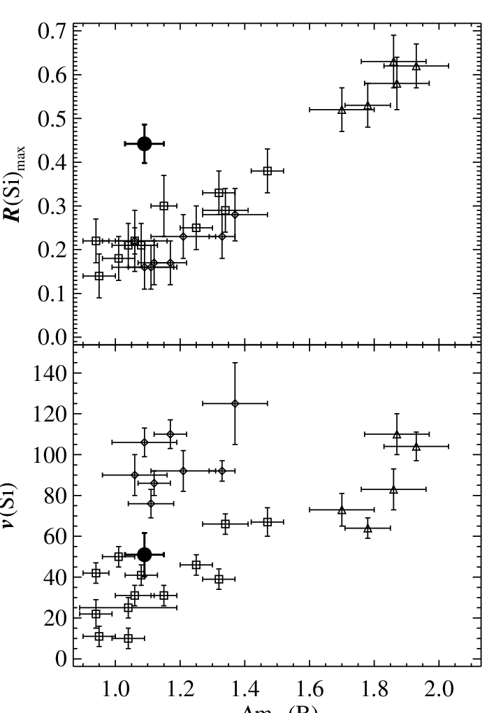
The true peculiar nature of SN 2006bt is apparent when comparing a temperature-dependent spectral parameter such as (Si) with a light-curve parameter such as . In Figure 7, we show these values for the sample of Benetti et al. [4] (open symbols) and for SN 2006bt (filled circle). In this parameter space, SN 2006bt is a large outlier, indicating that it has a relatively cool photosphere and a slow decline rate.
IV.5. Possible Detection of Carbon
In our earliest spectra, there is a small feature redward of Si II (see Figure 8). In our first spectrum (when the feature is strongest and the signal-to-noise ratio of the spectrum is highest), its minimum is at 6465 Å. This feature is present in our second and third spectra, although with less significance. These three spectra come from different instruments and telescopes, indicating that it is not an artifact of data reduction. The feature has mostly disappeared in our fourth spectrum ( days).

An intriguing possibility is that this feature is from C II absorption. If this is the case, the minimum of the absorption would be blueshifted by 5200 km s-1, which is much lower than that of other features and may indicate a misidentification. This feature has been detected in a handful of objects [9, e.g.,] with the best cases being SNe 2006D [59], 2006gz [29], and 2009dc [65], but all detections so far have been at much larger velocities and typically at much earlier phases. For instance, the minimum of the C II feature in SN 2006gz was blueshifted by 15,500 km s-1 at days (which was a larger velocity than the Si II feature at that phase) and had completely disappeared by days.
C II has four relatively strong features in the optical: , 4745, 6580, and 7234. Unfortunately, C II would be on the edge of a strong Mg II feature and C II is on top of a Ti II feature (although it may still be detectable with SYNOW; see Section IV.6). Only the two reddest lines are in relatively uncontaminated regions of the spectrum. As seen in Figure 8, there is a very shallow feature in our earliest spectrum at the wavelength that corresponds to C II blueshifted by 5000 km s-1.
Observations have shown that high-velocity features are common in SNe Ia [45, e.g.,]. The data can be explained by circumstellar interaction, dense blobs of material “detached” from the rest of the ejecta, or a differing covering fraction of the ejecta [23, 45, 58]. If there is a single carbon blob ejected at an angle away from our line of sight, the absorption velocity seen in the spectra would correspond to the component of the velocity vector along our line of sight. For an angle of 45∘ (65∘) relative to our line of sight, we infer a true velocity of 7450 km s-1 (12,300 km s-1) in such a scenario. This potential asymmetry may help explain other aspects of this SN (see Section VI.1). Alternatively, there may be a significant amount of carbon-rich material close to the SN. For this scenario, viewing-angle effects necessitate that our line of sight be in the plane of the circumstellar accretion disk.
Besides the possible detection of carbon lines, SN 2006bt shares other characteristics with SNe 2006D and 2006gz. SN 2006D had a relatively narrow light curve similar to that of SN 1986G, but not as narrow as that of SN 1991bg [59]. The day spectrum from Thomas et al. [59] is reproduced in Figure 5. The early-time spectra of SNe 2006D and 2006bt are relatively similar, both having relatively large (Si). SN 2006bt has slightly larger velocities for the Si and Ca features and stronger Ti II features than SN 2006D.
SN 2006gz had very broad light curves (), no shoulder in , and no second maximum in [29]. The colors were also very red, but Hicken et al. [29] attributed this to a large amount of host-galaxy extinction ( mag). SN 2006gz had spectra indicative of a very hot photosphere unlike SN 2006bt.
IV.6. SYNOW Model Fits
To investigate the details of our SN spectra, we use the supernova spectrum-synthesis code SYNOW [18]. Although SYNOW has a simple, parametric approach to creating synthetic spectra, it is a powerful tool to aid line identifications which in turn provide insights into the spectral formation of the objects. To generate a synthetic spectrum, one inputs a blackbody temperature (), a photospheric velocity (), and for each involved ion, an optical depth at a reference line, an excitation temperature (), the maximum velocity of the opacity distribution (), and a velocity scale (). This last variable assumes that the optical depth declines exponentially for velocities above with an -folding scale of . The strengths of the lines for each ion are determined by oscillator strengths and the approximation of a Boltzmann distribution of the lower-level populations with a temperature of .
In Figure 9, we present our day spectrum of SN 2006bt with a synthetic spectrum generated from SYNOW. This fit is very similar to the fit performed for SN 1986G by Branch et al. [8] and the optical depths for the fit are presented in Table 2. The main differences are that we include O I (it was excluded from the reference fit because of the short wavelength range of the SN 1986G spectrum), the excitation temperature is 8000 K instead of 7000 K, all ions other than Mg I and Mg II have lower optical depths, we do not include high-velocity Ca II and Fe II, and we do not impose a maximum velocity for Si II. The model includes low-ionization ions and excludes high-ionization ions, confirming the low-temperature nature of SN 2006bt. No ions at high velocity are included, further limiting the possibility of high-velocity ejecta. There are some differences between the SN 2006bt and SYNOW spectra. It is possible that these differences could be reduced by examining more of the parameter space of SYNOW input parameters. These differences do not affect our conclusions below.

| Value | ||||||||||||
|---|---|---|---|---|---|---|---|---|---|---|---|---|
| Parameter | C II | O I | Mg I | Mg II | Si II | S II | Ca I | Ca II | Sc II | Ti II | Co II | Ni II |
| 2 | 5 | 3 | 8 | 50 | 1 | 3 | 35 | 0.5 | 0.8 | 0.5 | 0.4 | |
A slightly higher excitation temperature and lower optical depths in SN 2006bt compared to SN 1986G is consistent with our relatively crude assessment of the spectrum in Section IV.2 where we considered SN 2006bt to be slightly hotter (and more “normal”) than SN 1986G. The model for SN 1986G has km s-1, while the model for SN 2006bt imposes no limit. Where nuclear burning may only extend to km s-1 in SN 1986G, it appears that it extends to all velocities in SN 2006bt.
Since we may have identified C II in the pre-maximum spectra of SN 2006bt (see Section IV.5), we created models with and without C II. In an attempt to match the possible low-velocity features, we included C II with K, km s-1, and km s-1. The inclusion of C II with these parameters improves the model fit. In addition to better fits near C II , 7234, the model is significantly better near C II . This shows that it is possible to detect lines in confused regions such as near 4600 Å. [8] fit this region with high-velocity Fe II, and again, we caution that the identification of C II is not definitive.
V. Supernova Environment
SN 2006bt occurred 33.7 kpc (, where is defined by the Petrosian radius where 50% of the flux is contained within a circle of radius ) from the nucleus of its host galaxy, CGCG 108-013, an S0/a galaxy (see Figure 10). SN 2006bt lies between its host and a nearby galaxy, 2MASX J15562803+2002482 (SN 2006bt is 23.7′′ east of the nucleus of 2MASX J15562803+2002482; although SN 2006bt lies between these two galaxies, we are confident that CGCG 108-013 is the host galaxy; see Section IV.1). This galaxy has , corresponding to a recession velocity that is 4250 km s-1 greater than that of CGCG 108-013 [1]. Examining SDSS images of the SN environment [1], there does not appear to be any tidal streams between the two galaxies. Although both objects are likely members of the Hercules supercluster, it is unlikely that they have interacted. There is another faint source 4.3′′ to the northwest (corresponding to 2.9 kpc at the redshift of CGCG 108-013) that has colors consistent with a background galaxy (with SDSS photo- of ; Csabai et al. 12) or a globular cluster. If it were a globular cluster at the redshift of CGCG 108-013, it would have mag, which is 2 mag brighter than G1 in M31. It is therefore more likely to be a background galaxy.

A spectrum of the nucleus of CGCG 108-013 from SDSS [1] shows no emission lines, suggesting little or no recent star formation. Using the single-stellar populations (SSP) models of Jimenez et al. [35], the spectrum of CGCG 108-013 is best fit by a population with a power-law initial mass function, an age of 14 Gyr, and a metallicity of 0.6 solar (see Figure 11). It is worth noting that Jimenez et al. [35] has no model with an age Gyr. Although such ages are limited by the age of the Universe, if the model ages are systematically larger than true ages, we may not be probing the full range of realistic models. Despite the excellent fit with an old SSP model, we cannot rule out additional (low-level) star formation over the past several Gyr.

Given the position of the SN, it is likely that the progenitor of SN 2006bt was a member of the halo population. If this were the case, then the progenitor would likely have formed before the majority of the stars in the bulge of the galaxy and with a lower metallicity. In this scenario, it is quite likely that the progenitor was of low metallicity and had an age of Gyr.
Alternatively, the progenitor may have formed in a galactic disk or the bulge and was ejected outward from an interaction with a supermassive black hole at the nucleus of the galaxy. To reach 33.7 kpc, the progenitor would have to travel at 3300, 330, 33, and 6.6 km s-1 for 10 Myr, 100 Myr, 1 Gyr, and 5 Gyr, respectively. From its position alone, it is very unlikely that the progenitor of SN 2006bt was a massive star () that formed near the galactic center and was ejected into the halo. It is possible that the progenitor was a low-mass star ejected in this manner, which would probably make it younger and have higher metallicity than other stars in the halo. Regardless, it is very likely that the progenitor of SN 2006bt was a white dwarf and SN 2006bt was not the result of some exotic core-collapse event.
VI. Discussion
VI.1. Models
It has long been believed that the vast majority of SN Ia light curves can be described by a single parameter which directly correlates with the amount of 56Ni produced in the explosion (with more 56Ni corresponding to more luminous events having broader light curves). Kasen & Woosley [38] explain this further by noting that objects with larger are hotter, making the recombination from Fe III to Fe II occur at a later time, and thus have a broader -band light curve.
Kasen [36] found that the depth of the trough, the height of the second maximum, and the delay between the first and second maxima in the band all increase with 56Ni mass. This finding would imply that SN 2006bt had a small 56Ni mass (model -band light curves with show a similar behavior to the -band light curve of SN 2006bt), which is in direct conflict with the decline rate of all bands.
The prominence of the second maximum is more generally related to the mass of all Fe-group elements in the ejecta, not just 56Ni and the isotopes into which it decays [36]. The second maximum can be reduced by decreasing the progenitor metallicity, which decreases the amount of stable Fe-group elements (“stable Fe”) produced in the explosion [60]; however, the effect is at most 10%. Since stable Fe is produced via electron capture, it is possible that the explosion simply did not have the physical conditions necessary to form a significant amount of stable Fe through electron capture. Finally, one can smear out the second maximum in by mixing the stable Fe and 56Ni throughout the ejecta [36]. This will also cause the maximum of the band to occur later, which may be the case for SN 2006bt.
SN 2006bt may have been a very asymmetric explosion. Although we see no indication of high-velocity ejecta in any of the spectral features, there is the possibility that a carbon blob was ejected 65∘ from our line of sight. SN 1999by, a low-luminosity event, showed a very polarized spectrum corresponding to an explosion with an asphericity of 20% viewed along the equator [32]. Asymmetric models show that peak luminosity depends on viewing angle; however, these models do not exhibit significant differences in ionization with viewing angle [37, 57].
It is also possible that SN 2006bt rose very quickly to maximum, causing a high luminosity with a smaller amount of 56Ni [3]. There are poor constraints on an explosion date from pre-explosion images [39]. Our photometry starts only a few days before maximum, but it does not appear to be faster than other objects with its decline rate. Although a fast rise is still a possibility, it appears to be an unlikely solution.
VI.2. Implications for Cosmology
Given its relatively normal luminosity, SN 2006bt-like objects would still be detected in high-redshift SN surveys, unlike other peculiar objects such as SNe 2002cx [41] and 2008ha [19, 61]. Furthermore, given its color curve, a SN 2006bt-like object with some host-galaxy extinction will simply look like a normal object with that extinction plus an additional mag of extinction. At some point too much extinction would lead to the exclusion of these objects from a SN sample; most cosmological analyses avoid SNe Ia having extremely red colors.
Additionally, at high redshift, the rest-frame and band will be redshifted out of the optical, requiring observers to rely on rest-frame alone to determine the quality of the light-curve fits and measure the extinction. At low redshift, one could search for objects with large but no secondary maximum in and exclude any such objects; however, at high redshift this is not feasible without observing in the near infrared (JWST and, depending on the ultimately chosen design, JDEM might be able to measure the rest-frame band out to ). For an object at (where is redshifted out of the optical), one would have to rely on a spectrum (in combination with a light curve) to identify SN 2006bt-like objects. However, with the Si II lines redshifting out of the optical window at and the generally low signal-to-noise ratio spectra of high-redshift SNe Ia, it is difficult to detect spectroscopically peculiar objects from high-redshift surveys [21].
If SN 2006bt does come from a very old progenitor and the age of the progenitor is the main reason for its peculiarity, then SN 2006bt-like objects may not exist at high redshift. At and 1, the Universe had an age of 8.6 and 5.9 Gyr, respectively. If the delay time between formation and explosion is longer than those times, SN 2006bt-like objects will not exist at those redshifts. Foley et al. [21] found no SN 1991bg-like objects in a sample of 118 high-redshift SNe Ia, indicating that SN 2006bt-like objects are probably not a large fraction of the early-universe SN Ia population.
We have developed a Monte Carlo simulation to assess the impact of contamination of a population of SN 2006bt-like objects in a SN Ia cosmological sample. For normal SNe Ia, we generate 1000 light curves over a range of light-curve shape parameters from the MLCS2k2 “early” templates [34] over (500 for and 500 for ), with distance modulus, , calculated in a nominal flat CDM (, ) cosmology. We parameterize the input extinction by a O’Donnell [49] law, with drawn from the glos distribution [27, e.g.,]. The light-curve shape parameter is drawn randomly between and 1.3. The sampling and signal-to-noise ratio is matched to the expected values for the Pan-STARRS Medium Deep Survey.
Since SN 2006bt has very different light curves from those of other SNe Ia, the MLCS2k2 template light curves had to be modified to create simulated light curves of SN 2006bt-like objects. Specifically, the SN 2006bt-like light curves must be intrinsically underluminous and red compared to a nominal SN Ia with the same light-curve shape. To determine the appropriate modifications, each individual light curve of SN 2006bt was fit separately. The light curves all had best fits of , while the -band light curve was best fit with . The MLCS2k2 model light curves were shifted so that the peak magnitudes were the same as those of SN 2006bt in each band. We created 100 SN 2006bt-like light curves for (50 for and 50 for ).
All light curves were fit using MLCS2k2 [34], which provided estimates of , , and . The fitting was performed with both the glos and flatnegav (a flat prior which includes negative values of ) priors. Fits of all light curves, including those for SN 2006bt-like objects, had a reduced , indicating that all would nominally be included in a cosmological analysis.
To demonstrate how MLCS2k2 interprets our SN 2006bt-like model light curves as a function of redshift, we produced noise-free light curves spanning the redshift interval . The light curves were fit by MLCS2k2 with a flatnegav prior (in this signal-to-noise ratio regime, the prior is inconsequential and the uncertainty is dominated by the MLCS model uncertainty). The resulting distance modulus residuals and derived are presented in Figure 12. The derived distance modulus residuals are close to zero near , but increase to 0.1 mag at . After that, the residuals generally linearly decrease with increasing redshift, deviating by 0.5 mag at . At redshifts where either the mapping of observed filters to rest-frame filters during the K-correction process changes or when a rest-frame filter is no longer used in K-corrections (the filter “drops out”), there are large discontinuities in the residuals. These discontinuities are partly the result of our model for SN 2006bt and the normal SN Ia template model and partly the result of having the observer-frame light curves derived from a single rest-frame filter.

The derived value for has a very similar (but inverted) function with redshift. Since our model assumes mag at all redshifts, the derived value corresponds to the difference between the true distance modulus and the derived distance modulus, modulo the difference in peak absolute magnitude for SN 2006bt and the canonical SN Ia with the same . Although the distance modulus residuals appear to be quite large, the distance modulus is compared to the input cosmological model. When fitting an observed sample, one can only look for outliers from the best fit, and the inclusion of SN 2006bt-like objects will influence such a fit. Furthermore, a deviation of a few tenths of a magnitude from the residual of the best-fit cosmology is expected for several objects in a high-redshift SN sample.
To examine the impact of SN 2006bt-like objects on cosmological parameter estimation, we defined 7 distinct samples. The first sample had no contamination from SN 2006bt-like objects. The remaining samples had 1%, 5%, or 10% contamination at all redshifts, or only for (consistent with a very long delay time for such objects). The distance moduli found using MLCS2k2 were used to constrain the cosmological parameters and with the assumption of flatness. We also combined the SN data with the prior from the baryon acoustic oscillations [13, BAO;], further constraining the cosmological parameters. Since we fit the light curves using two separate extinction priors, we have a total of 14 different estimates of and with and without BAO constraints. The parameters are listed in Table 3.
| Sample | (SNe Only) | (SNe + BAO) | (SNe Only) | (SNe + BAO) |
|---|---|---|---|---|
| flatnegav Prior | ||||
| No contamination | ||||
| 1% contamination | ||||
| 5% contamination | ||||
| 10% contamination | ||||
| 1% contamination low- | ||||
| 5% contamination low- | ||||
| 10% contamination low- | ||||
| glos Prior | ||||
| No contamination | ||||
| 1% contamination | ||||
| 5% contamination | ||||
| 10% contamination | ||||
| 1% contamination low- | ||||
| 5% contamination low- | ||||
| 10% contamination low- | ||||
Note. — BAO alone results in and . Since the input cosmology of and differs slightly from this best-fit result, there is some tension between the datasets and their combination will cause the combined contours to move toward the BAO-only results.
As SN 2006bt-like objects become a larger share of the SN sample, the estimate of consistently increases (becoming closer to 0). The value derived from the uncontaminated sample is and for the glos and flatnegav priors, respectively, while the the 10% contaminated (at all redshifts) sample yields and for the same priors, respectively. This trend is true if the SN 2006bt-like objects are spread throughout redshift or restricted only to low redshifts, but which of these two samples has more bias depends on the prior. For the SN-only cosmological fits, the value of is typically biased to lower values, but only the fits with the glos prior are substantially biased. The 1 contours for the uncontaminated and 10% contaminated samples are shown in Figure 13.

From our basic simulations, we see that SN 2006bt-like objects can have a large impact on derived cosmological parameters; however, if the fraction of SN 2006bt-like objects in the sample is low, the bias can be much smaller than other systematic biases (if 1% of the low-redshift sample in contaminated by SN 2006bt-like objects, shifts by only 0.007). We have identified one object with these peculiar properties out of 185 objects in the CfA3 sample, but we have not examined all objects with the same scrutiny. Within the CfA3 sample, 20% of SNe Ia have measured larger than that of SN 2006bt, which is a very conservative upper bound to the fraction of the contamination of the low-redshift sample.
VII. Conclusions
SN 2006bt is a unique object that defies the conventional wisdom of how SN Ia observables should correlate. SN 2006bt has slowly declining light curves, but its spectra indicate a cool photosphere. The combination of the broad light curves and intrinsic red colors causes light-curve fitters to indicate that SN 2006bt is heavily reddened. The object is a slight outlier to the WLR. Although SN 2006bt is underluminous for its light-curve shape, light-curve fitters correct for this in a way that estimates a distance modulus that is very close to the Hubble-flow value.
We discovered the peculiar nature of SN 2006bt by noticing that it had a large derived extinction value for its PGCD, but this was after 30 included SN 2006bt in a cosmological analysis. We may find similar objects by looking for comparable outliers, but it is also possible to find SN 2006bt-like objects by examining their light curves and spectra. SN 2006bt is a clear outlier in the relationship between and (Si). Unlike SNe Ia with similar decline raters, SN 2006bt lacks a prominent second maximum in the band. Both of these observables could be used to find additional examples.
There are spectroscopic features which are consistent with C II, but at a significantly lower velocity than other spectral features. If these features are caused by carbon, it can be explained by a carbon blob ejected 65∘ from our line of sight.
The SN position and the host-galaxy type and spectrum indicate that SN 2006bt had a very old progenitor. If a very old progenitor is necessary to create a SN 2006bt-like event, we may not expect to find any similar objects at high redshift.
Contamination of SN 2006bt-like objects in samples of SNe Ia used for cosmological analyses is a potential source of a large bias in the determination of and . If these objects are only 1% of the low-redshift sample (similar to the sample used by 30), then the bias should be in . However, if these objects are a larger percentage of the sample, this could be the dominant systematic uncertainty for SN cosmology. It seems unlikely that SN 2006bt-like objects are more than a few percent of the local sample, but it is much harder to characterize similar objects at high redshift (where the rest-frame band is not observed, and low signal-to-noise ratio spectra may not cover the Si II feature). Future studies should attempt to identify SN 2006bt-like objects and exclude them from cosmological analyses.
References
- [1] Abazajian, K. N., et al. 2009, ApJS, 182, 543
- [2] Aldering, G., et al. 2006, ApJ, 650, 510
- [3] Arnett, W. D. 1982, ApJ, 253, 785
- [4] Benetti, S., et al. 2005, ApJ, 623, 1011
- [5] ——. 2004, MNRAS, 348, 261
- [6] Blondin, S., & Tonry, J. L. 2007, ApJ, 666, 1024
- [7] Branch, D., Dang, L. C., & Baron, E. 2009, PASP, 121, 238
- [8] Branch, D., et al. 2006, PASP, 118, 560
- [9] ——. 2003, AJ, 126, 1489
- [10] Colgate, S. A., & McKee, C. 1969, ApJ, 157, 623
- [11] Conley, A., Carlberg, R. G., Guy, J., Howell, D. A., Jha, S., Riess, A. G., & Sullivan, M. 2007, ApJ, 664, L13
- [12] Csabai, I., et al. 2003, AJ, 125, 580
- [13] Eisenstein, D. J., et al. 2005, ApJ, 633, 560
- [14] Fabricant, D., Cheimets, P., Caldwell, N., & Geary, J. 1998, PASP, 110, 79
- [15] Filippenko, A. V., & Foley, R. J. 2006, Central Bureau Electronic Telegrams, 485, 2
- [16] Filippenko, A. V., et al. 1992a, AJ, 104, 1543
- [17] ——. 1992b, ApJ, 384, L15
- [18] Fisher, A., Branch, D., Nugent, P., & Baron, E. 1997, ApJ, 481, L89+
- [19] Foley, R. J., et al. 2009a, AJ, 138, 376
- [20] Foley, R. J., Filippenko, A. V., & Jha, S. W. 2008, ApJ, 686, 117
- [21] Foley, R. J., et al. 2009b, AJ, 137, 3731
- [22] ——. 2003, PASP, 115, 1220
- [23] Gerardy, C. L., et al. 2004, ApJ, 607, 391
- [24] Guy, J., et al. 2007, A&A, 466, 11
- [25] Hachinger, S., Mazzali, P. A., Tanaka, M., Hillebrandt, W., & Benetti, S. 2008, MNRAS, 389, 1087
- [26] Hamuy, M., et al. 2003, Nature, 424, 651
- [27] Hatano, K., Branch, D., & Deaton, J. 1998, ApJ, 502, 177
- [28] Hicken, M., et al. 2009a, ApJ, 700, 331
- [29] Hicken, M., Garnavich, P. M., Prieto, J. L., Blondin, S., DePoy, D. L., Kirshner, R. P., & Parrent, J. 2007, ApJ, 669, L17
- [30] Hicken, M., Wood-Vasey, W. M., Blondin, S., Challis, P., Jha, S., Kelly, P. L., Rest, A., & Kirshner, R. P. 2009b, ApJ, 700, 1097
- [31] Horne, K. 1986, PASP, 98, 609
- [32] Howell, D. A., Höflich, P., Wang, L., & Wheeler, J. C. 2001, ApJ, 556, 302
- [33] Howell, D. A., et al. 2006, Nature, 443, 308
- [34] Jha, S., Riess, A. G., & Kirshner, R. P. 2007, ApJ, 659, 122
- [35] Jimenez, R., MacDonald, J., Dunlop, J. S., Padoan, P., & Peacock, J. A. 2004, MNRAS, 349, 240
- [36] Kasen, D. 2006, ApJ, 649, 939
- [37] Kasen, D., & Plewa, T. 2007, ApJ, 662, 459
- [38] Kasen, D., & Woosley, S. E. 2007, ApJ, 656, 661
- [39] Lee, E., & Li, W. 2006, Central Bureau Electronic Telegrams, 485, 1
- [40] Leibundgut, B., et al. 1993, AJ, 105, 301
- [41] Li, W., et al. 2003, PASP, 115, 453
- [42] ——. 2001, PASP, 113, 1178
- [43] Lira, P., et al. 1998, AJ, 115, 234
- [44] Matheson, T., et al. 2008, AJ, 135, 1598
- [45] Mazzali, P. A., et al. 2005, ApJ, 623, L37
- [46] Miller, J. S., & Stone, R. P. S. 1993, Lick Obs. Tech. Rep. 66 (Santa Cruz: Lick Obs.)
- [47] Nomoto, K., Thielemann, F.-K., & Yokoi, K. 1984, ApJ, 286, 644
- [48] Nugent, P., Phillips, M., Baron, E., Branch, D., & Hauschildt, P. 1995, ApJ, 455, L147
- [49] O’Donnell, J. E. 1994, ApJ, 422, 158
- [50] Oke, J. B., et al. 1995, PASP, 107, 375
- [51] Phillips, M. M. 1993, ApJ, 413, L105
- [52] Phillips, M. M., et al. 2007, PASP, 119, 360
- [53] Phillips, M. M., Lira, P., Suntzeff, N. B., Schommer, R. A., Hamuy, M., & Maza, J. 1999, AJ, 118, 1766
- [54] Phillips, M. M., et al. 1987, PASP, 99, 592
- [55] Phillips, M. M., Wells, L. A., Suntzeff, N. B., Hamuy, M., Leibundgut, B., Kirshner, R. P., & Foltz, C. B. 1992, AJ, 103, 1632
- [56] Schlegel, D. J., Finkbeiner, D. P., & Davis, M. 1998, ApJ, 500, 525
- [57] Sim, S. A., Sauer, D. N., Röpke, F. K., & Hillebrandt, W. 2007, MNRAS, 378, 2
- [58] Tanaka, M., Mazzali, P. A., Maeda, K., & Nomoto, K. 2006, ApJ, 645, 470
- [59] Thomas, R. C., et al. 2007, ApJ, 654, L53
- [60] Timmes, F. X., Brown, E. F., & Truran, J. W. 2003, ApJ, 590, L83
- [61] Valenti, S., et al. 2009, Nature, 459, 674
- [62] Wade, R. A., & Horne, K. 1988, ApJ, 324, 411
- [63] Wang, X., et al. 2009, ApJ, 699, L139
- [64] Whelan, J., & Iben, I. J. 1973, ApJ, 186, 1007
- [65] Yamanaka, M., et al. 2009, ArXiv e-prints, 0908.2059