跳到论文正文
W Papers独立论文阅读器 arXiv:0912.0199 论文正文 计算阅读时间 · 0%
引用这篇论文根据当前论文元数据生成,正式投稿前建议核对。


License: arXiv.org perpetual non-exclusive license
arXiv:0912.0199v4 [hep-ph] 26 Mar 2010

Next-to-leading order QCD predictions for graviton and photon associated production in the Large Extra Dimensions model at the LHC

Xiangdong Gao Address: Department of Physics and State Key Laboratory of Nuclear Physics and Technology, Peking University, Beijing 100871, China    Chong Sheng Li Email: csli@pku.edu.cn Address: Department of Physics and State Key Laboratory of Nuclear Physics and Technology, Peking University, Beijing 100871, China    Jun Gao Address: Department of Physics and State Key Laboratory of Nuclear Physics and Technology, Peking University, Beijing 100871, China    Robert J. Oakes Address: Department of Physics and Astronomy, Northwestern University, Evanston, Illinois, 60208-3112, USA    Jian Wang Address: Department of Physics and State Key Laboratory of Nuclear Physics and Technology, Peking University, Beijing 100871, China
August 24, 2026
Abstract

We present the calculations of the complete next-to-leading order(NLO) QCD corrections to the inclusive total cross sections for the Kaluza-Klein(KK) graviton and photon associated production process p​p→γ​GK​K+Xpp\rightarrow\gamma G_{KK}+X in the large extra dimensions model at the LHC. We show that the NLO QCD corrections in general enhance the total cross sections and reduce the dependence of the total cross sections on the factorization and renormalization scales. When jet veto is considered, the NLO corrections reduce the total cross sections. We also calculate some important differential cross sections for this process at NLO: the missing transverse momentum distribution, the transverse momentum distribution and the pseudorapidity distribution of photon.

pacs
11.10.Kk, 12.38.Bx, 13.85.Qk, 14.80.Rt

I introduction

The idea that the extra dimensions theory can appear at the TeV scale, well below the Planck scale MP∼1.2×10¹⁹M_{P}\sim 1.2\times 10^{19}GeV, was proposed in the 1990s[1, 2, 3, 4, 5, 6, 7, 8, 9, 10] and promises rich phenomenology at the TeV scale. Now the search for extra dimensions is one of the important tasks for the LHC.

Among various extra dimensions models the large extra dimensions(LED) model introduced in Ref.[1, 2, 3] is the first TeV scale gravity theory and has been extensively studied[11, 12]. In this model space-time has 4+δ4+\delta dimensions and the standard model(SM) particles reside in the usual 3+13+1-dimensional SM brane and can not propagate in the extra δ\delta-dimensional space, which is assumed to be compacted on a torus with a common radius RR, while gravity can propagate in the whole 4+δ4+\delta dimensional world. From the view of our 4-dimensional world, there exists infinitely many Kaluza-Klein(KK) modes of gravitons with mass |k|/R|k|/R interacting with SM particles, where k2=∑i=1δki2k^{2}=\sum_{i=1}^{\delta}k_{i}^{2} with kik_{i} being the integer. The 4-dimensional Planck scale is no longer the fundamental scale, but an effective scale in the 4-dimensional world, and is related to a fundamental scale MD∼M_{D}\simTeV by the Newtonian law of gravitation in 4+δ4+\delta dimensions[1, 12]

M¯P≡MP/8​π=Rδ/2​MD1+δ/2,\bar{M}_{P}\equiv M_{P}/\sqrt{8\pi}=R^{\delta/2}M_{D}^{1+\delta/2}, (1)

where M¯P\bar{M}_{P} is the reduced Planck mass. According to Eq.(1), deviations from the usual Newtonian gravitational law appear at R∼1032δ−19R\sim 10^{\frac{32}{\delta}-19} meters, which is not a conflict with the current gravitational experiments[13] once δ≥2\delta\geq 2. Before further results of terrestrial gravitational experiments appear, one may resort to colliders to find signals of this model. Although, in this model the couplings of gravitons to SM particles are suppressed by 1/MP1/M_{P} [11, 12], the summation of the production of large numbers of KK modes with arbitrary mass smaller than MDM_{D} may compensate for this suppression and lead to observable effects. There are two ways to probe such effects at colliders: graviton emission and virtual graviton exchange, which have been investigated in Ref. [12, 11, 14]. As shown in Ref.[12], because of the suppression of the couplings of gravitons to SM particles, the decays of gravitons to SM particles have a small probability to occur before they propagate into the extra δ\delta-dimensional space, which means the gravitons behave like massive, stable, and noninteracting particles once they are produced. Thus, the signal for graviton and photon associated production at the LHC is a single photon plus missing energy. Since the electromagnetic coupling is small and the q​q¯q\bar{q} luminosity is lower than for g​ggg at the LHC the rate for this process is much smaller than for jet and graviton associated production. But the photon signal would be a clean signature; and in case of discovery in jet plus graviton events, the photon plus graviton signal would provide a useful independent test[12]. Only leading-order(LO) calculations and analysis of the process were performed in Ref.[12]. Since LO cross sections for processes at hadron colliders suffer from large uncertainties due to the choices of the renormalization scale (μr\mu_{r}) and factorization scale (μf\mu_{f}) and higher order QCD corrections are generally large and can improve the scale uncertainties at hadron colliders. Several works[15, 16, 17, 18, 19, 20, 21, 22, 23] have performed next-to-leading order(NLO) QCD corrections in extra dimensions models. In this paper we present the complete calculations of NLO QCD corrections to this process which improve the theoretical predictions.

This paper is organized as follows. In Sec.II we show the analytic results of the LO calculations and define the notation. In Sec.III we present the details of the calculations of both the virtual and real parts of the NLO QCD corrections. In Sec.IV we give the numerical predictions for inclusive and differential cross sections at the LHC. We close this paper with a brief conclusion. For completeness, the relevant Feynman rules are collected in Appendix A and the lengthy analytic expressions of the results of our calculations are summarized in Appendix B.

II Leading-order calculations

The KK gravitons with different masses can be produced at colliders only if kinematically allowed. Contributions from the different KK modes then must be summed up. Since the KK graviton mass separation of 𝒪⁡(1/R)\mathcal{O}(1/R) is much smaller than all the other physical scales involved, we can replace the discrete summation of different KK modes by a continuous integration. In general, the differential cross section for graviton production can be expressed as[12]

d2​σd​t​d​m=Sδ−1​M¯P2MD2+δ​mδ−1​d​σmd​t\frac{d^{2}\sigma}{dt~dm}=S_{\delta-1}\frac{\bar{M}^{2}_{P}}{M^{2+\delta}_{D}}m^{\delta-1}\frac{d\sigma_{m}}{dt} (2)

with

Sδ−1=2​πδ/2Γ⁡(δ/2),S_{\delta-1}=\frac{2\pi^{\delta/2}}{\Gamma(\delta/2)}, (3)

where Sδ−1S_{\delta-1} is the surface of a unit-radius sphere in δ\delta dimensions and d​σm/d​td\sigma_{m}/dt is the differential cross section for producing a single KK graviton of mass mm. Throughout this work we perform the integration on mm from 0.1​MD0.1M_{D} to MDM_{D}.

Refer to caption
Figure 1: Leading-order Feynman diagrams for q​q¯→γ​GK​Kq\bar{q}\rightarrow\gamma G_{KK}.

The leading-order Feynman diagrams for the graviton and photon associated production process q⁡(p1)​q¯​(p2)→γ⁡(p3)​GK​K​(p4)q(p_{1})\bar{q}(p_{2})\rightarrow\gamma(p_{3})G_{KK}(p_{4}) are shown in Fig. 1. The related Feynman rules are given in Ref. [11, 12] and are collected in Appendix A. The LO amplitudes have been given in Ref.[11] so we need only to show the amplitudes squared here. In the LED model the spin sum over the polarization tensors of the graviton is

∑5s=1ϵsμ​νϵs∗α​β=Pμ​ν​α​β,\sum^{5}_{s=1}\epsilon^{s}_{\mu\nu}\epsilon^{s\ast}_{\alpha\beta}=P_{\mu\nu\alpha\beta}, (4)

with

Pμ​ν​α​β=ημ​α​ην​β+ημ​β​ημ​α−2n−1​ημ​ν​ηα​β+…,P_{\mu\nu\alpha\beta}=\eta_{\mu\alpha}\eta_{\nu\beta}+\eta_{\mu\beta}\eta_{\mu\alpha}-\frac{2}{n-1}\eta_{\mu\nu}\eta_{\alpha\beta}+..., (5)

where the dots represent terms proportional to the graviton momentum p4μp^{\mu}_{4} and p4μ​Tμ​ν=0p^{\mu}_{4}T_{\mu\nu}=0, giving no contribution to the amplitude. We performed our calculations in n=4−2​ϵn=4-2\epsilon dimensions.

The LO partonic cross section is then

σ^mB=12​s​∫d​Γ2​∑¯​|MB|2,\hat{\sigma}_{m}^{B}=\frac{1}{2s}\int d\Gamma_{2}\overline{\sum}|M^{B}|^{2}, (6)

with

∑¯​|MB|2\displaystyle\overline{\sum}|M^{B}|^{2} =\displaystyle= eQ2​κ224​s​t​u[(s+4t)m6−6t(s+2t)m4+(s3+6ts2+18t2s+16t3)m2\displaystyle\frac{\text{eQ}^{2}\kappa^{2}}{24stu}\left[(s+4t)m^{6}-6t(s+2t)m^{4}+\left(s^{3}+6ts^{2}+18t^{2}s+16t^{3}\right)m^{2}\right. (7)
−4t(s3+3ts2+4t2s+2t3)],\displaystyle\left.-4t\left(s^{3}+3ts^{2}+4t^{2}s+2t^{3}\right)\right],

where κ=2/M¯P\kappa=\sqrt{2}/\bar{M}_{P}, ss, tt, and uu are the Mandelstam variables defined as

s=(p1+p2)2,t=(p1−p3)2,u=(p1−p4)2,s=(p_{1}+p_{2})^{2},~~~t=(p_{1}-p_{3})^{2},~~~u=(p_{1}-p_{4})^{2}, (8)

and ∑¯\overline{\sum} means that the colors and spins of the outgoing particles have been summed over and the colors and spins of the incoming particles have been averaged over. Equation(7) is a coincidence with the result shown in Ref.[12].

The LO total cross section can be obtained by convoluting the partonic cross sections with the parton distribution functions(PDF) Gq,q¯G_{q,\bar{q}} in the protons:

σmB=∫d​x1​d​x2​[Gq/p​(x1,μf)​Gq¯/p​(x2,μf)+Gq/p​(x2,μf)​Gq¯/p​(x1,μf)]​σ^mB.\sigma^{B}_{m}=\int dx_{1}dx_{2}[G_{q/p}(x_{1},\mu_{f})G_{\bar{q}/p}(x_{2},\mu_{f})+G_{q/p}(x_{2},\mu_{f})G_{\bar{q}/p}(x_{1},\mu_{f})]\hat{\sigma}_{m}^{B}. (9)

Here μf\mu_{f} is the factorization scale.

III Next-to-leading order calculations

The NLO corrections to the associated production of a graviton and a photon can be separated into the virtual corrections arising from loop diagrams of colored particles and the real corrections arising from the radiation of a real gluon or a massless (anti)quark. We carried out the calculations in the ’t Hooft-Feynman gauge and used dimensional regularization[24] in n=4−2​ϵn=4-2\epsilon dimensions to regulate all the ultraviolet(UV), soft and collinear divergences. We performed two independent calculations for both the analytical and numerical results for cross checking, and the results of the two groups agree with each other.

III.1 Virtual corrections

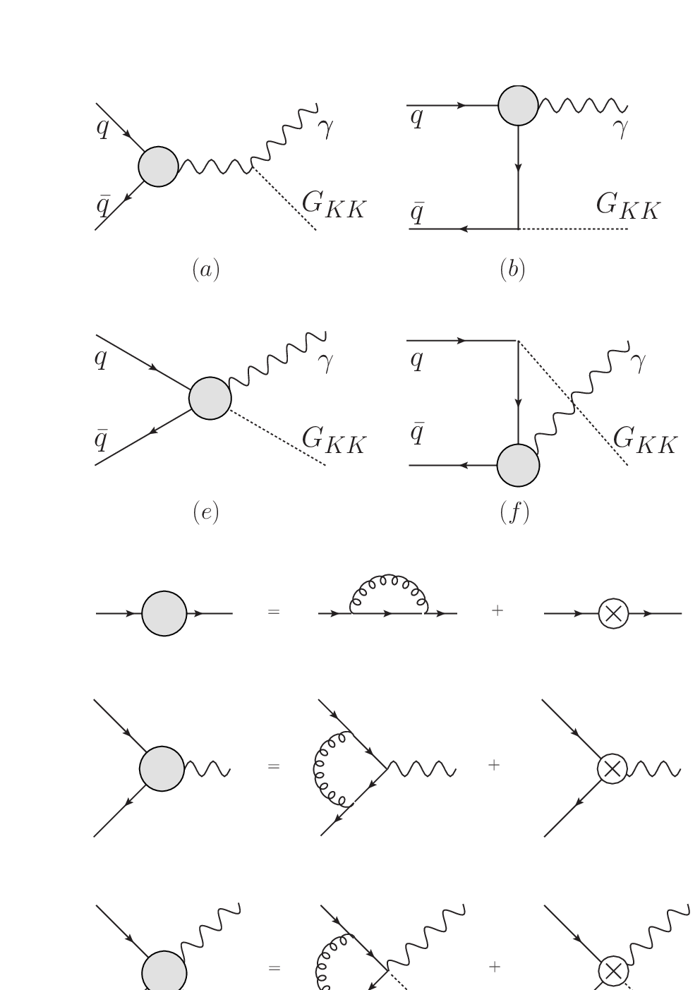
The Feynman diagrams for the virtual corrections to q​q¯→γ​GK​Kq\bar{q}\rightarrow\gamma G_{KK} are shown in Fig.2 and Fig.3. They consist of self-energy, vertex, triangle and box diagrams. In order to remove the UV divergence we adopt the on-shell renormalization scheme[25, 26, 27, 28].

We denote the bare and renormalized quark wave functions by ψq​0\psi_{q0} and ψq\psi_{q}, respectively. The renormalization constant δ​Zq\delta Z_{q} is then defined by

ψq​0=(1+δ​Zq)1/2​ψq.\psi_{q0}=(1+\delta Z_{q})^{1/2}\psi_{q}. (10)

Calculating the quark self-energy diagram we obtain the explicit expression for δ​Zq\delta Z_{q}:

δ​Zq=αs4​π​CF​(1ϵ−1ϵU​V).\delta Z_{q}=\frac{\alpha_{s}}{4\pi}C_{F}(\frac{1}{\epsilon}-\frac{1}{\epsilon_{UV}}). (11)

Here CF=43C_{F}=\frac{4}{3} while 1/ϵ1/\epsilon and 1/ϵU​V1/\epsilon_{UV} represent infrared(IR) and UV divergences, respectively.

After renormalization the UV divergences in the virtual corrections are removed leaving the IR divergences and the finite terms. The 𝒪⁡(αs)\mathcal{O}(\alpha_{s}) virtual corrections to the partonic total cross section can then be expressed as

σ^mV=12​s​∫d​Γ2​∑¯​[αs2​π​Γ⁡(1−ϵ)Γ⁡(1−2​ϵ)​(4​π​μr2s)ϵ​(2​A2Vϵ2+2​A1Vϵ)​|MB|2+αs2​π​𝒮],\hat{\sigma}^{V}_{m}=\frac{1}{2s}\int d\Gamma_{2}\overline{\sum}\left[\frac{\alpha_{s}}{2\pi}\frac{\Gamma(1-\epsilon)}{\Gamma(1-2\epsilon)}\left(\frac{4\pi\mu^{2}_{r}}{s}\right)^{\epsilon}\left(\frac{2A^{V}_{2}}{\epsilon^{2}}+\frac{2A^{V}_{1}}{\epsilon}\right)|M^{B}|^{2}+\frac{\alpha_{s}}{2\pi}\mathcal{S}\right], (12)

with

A2V=−CF,A1V=−32​CF.A^{V}_{2}=-C_{F},~~~A^{V}_{1}=-\frac{3}{2}C_{F}. (13)

Here 𝒮\mathcal{S} represents finite terms in the virtual corrections and the explicit expressions are given in Appendix B. The cancellation of IR divergent terms 1/ϵ21/{\epsilon^{2}} and 1/ϵ1/\epsilon will be discussed in detail below.

Refer to caption
Figure 2: One-loop virtual diagrams including vertex and self-energy corrections to q​q¯→γ​GK​Kq\bar{q}\rightarrow\gamma G_{KK}. Each brown vertex is UV divergence free.
Refer to caption
Figure 3: Box and triangle diagrams for q​q¯→γ​GK​Kq\bar{q}\rightarrow\gamma G_{KK}. The UV divergences cancel among the five diagrams.

III.2 Real gluon emission

The Feynman diagrams for the real gluon emission process q⁡(p1)​q¯​(p2)→γ⁡(p3)​GK​K​(p4)+g⁡(p5)q(p_{1})\bar{q}(p_{2})\rightarrow\gamma(p_{3})G_{KK}(p_{4})+g(p_{5}) are shown in Fig. 4.

The phase space integration for the real gluon emission will produce soft and collinear singularities which can be conventionally isolated by slicing the phase space into different regions using suitable cutoffs. In this paper we use the two-cutoff phase space slicing method[29], which introduces two arbitrary small cutoffs; i.e., a soft cutoff δs\delta_{s} and a collinear cutoff δc\delta_{c}, to divide the three-body phase space into three regions.

First, the phase space is separated into two regions by the soft cutoff δs\delta_{s}, according to whether the energy of the emitted gluon is soft; i.e., E5≤δs​s/2E_{5}\leq\delta_{s}\sqrt{s}/2, or hard; i.e., E5>δs​s/2E_{5}>\delta_{s}\sqrt{s}/2. Then the parton level real cross section σ^mR\hat{\sigma}^{R}_{m} can be written as

σ^mR=σ^mS+σ^mH,\displaystyle\hat{\sigma}^{R}_{m}=\hat{\sigma}^{S}_{m}+\hat{\sigma}^{H}_{m}, (14)

where σ^mS\hat{\sigma}^{S}_{m} and σ^mH\hat{\sigma}^{H}_{m} are the contributions from the soft and hard regions, respectively. σ^mS\hat{\sigma}^{S}_{m} contains all the soft divergences, which can explicitly be obtained after the integration over the phase space of the emitted gluon. Next, in order to isolate the remaining collinear divergences from σ^mH\hat{\sigma}^{H}_{m}, the collinear cutoff δc\delta_{c} is introduced to further split the hard gluon phase space into two regions, according to whether the Mandelstam variables ti​5≡(pi−p5)2t_{i5}\equiv(p_{i}-p_{5})^{2}, with i=1,2i=1,2, satisfy the collinear condition −δc​s<ti​5<0-\delta_{c}s<t_{i5}<0 or not. We then have

σ^mH=σ^mH​C+σ^mH​C¯,\displaystyle\hat{\sigma}^{H}_{m}=\hat{\sigma}^{HC}_{m}+\hat{\sigma}^{\overline{HC}}_{m}, (15)

where the hard collinear part σ^mH​C\hat{\sigma}^{HC}_{m} contains the collinear divergences, which also can explicitly be obtained after the integration over the phase space of the emitted gluon. The hard noncollinear part σ^mH​C¯\hat{\sigma}^{\overline{HC}}_{m} is finite and can be numerically computed using standard Monte Carlo integration techniques[30] and can be written in the form

d​σ^mH​C¯=12​s​∑¯​|Mq​q¯|2​d​Γ¯3.\displaystyle d\hat{\sigma}^{\overline{HC}}_{m}=\frac{1}{2s}\overline{\sum}|M^{q\bar{q}}|^{2}d\overline{\Gamma}_{3}. (16)

Here d​Γ¯3d\overline{\Gamma}_{3} is the hard noncollinear region of the three-body phase space.

In the next two subsections we will discuss in greater detail the soft and hard collinear gluon emission.

III.2.1 Soft gluon emission

In the limit that the energy of the emitted gluon becomes small, i.e. E5≤δs​s/2E_{5}\leq\delta_{s}\sqrt{s}/2, the amplitude squared ∑¯​|M⁡(q​q¯→γ​GK​K+g)|2\overline{\sum}|M(q\bar{q}\to\gamma G_{KK}+g)|^{2} can be factorized into the Born amplitude squared times an eikonal factor Φeik\Phi_{\text{eik}}:

∑¯​|M⁡(q​q¯→γ​GK​K+g)|2⟶soft(4​π​αs​μr2​ϵ)​∑¯​|MB|2​Φeik,\overline{\sum}|M(q\bar{q}\to\gamma G_{KK}+g)|^{2}\stackrel{{\scriptstyle\text{soft}}}{{\longrightarrow}}(4\pi\alpha_{s}\mu_{r}^{2\epsilon})\overline{\sum}|M^{B}|^{2}\Phi_{\text{eik}}, (17)

where the eikonal factor is given by

Φeik=CF​s(p1⋅p5)​(p2⋅p5).\Phi_{\text{eik}}=C_{F}\frac{s}{(p_{1}\cdot p_{5})(p_{2}\cdot p_{5})}. (18)

Moreover, the three-body phase space in the soft limit can also be factorized:

d​Γ3​(q​q¯→γ​GK​K+g)⟶softd​Γ2​(q​q¯→γ​GK​K)​d​S.d\Gamma_{3}(q\bar{q}\to\gamma G_{KK}+g)\stackrel{{\scriptstyle\text{soft}}}{{\longrightarrow}}d\Gamma_{2}(q\bar{q}\to\gamma G_{KK})dS. (19)

Here d​SdS is the integration over the phase space of the soft gluon and is given by[29]

𝑑S=12​(2​π)3−2​ϵ​∫0δs​s/2d​E5​E51−2​ϵ​d​Ω2−2​ϵ.dS=\frac{1}{2(2\pi)^{3-2\epsilon}}\int^{\delta_{s}\sqrt{s}/2}_{0}dE_{5}E_{5}^{1-2\epsilon}d\Omega_{2-2\epsilon}. (20)

The parton level cross section in the soft region can then be expressed as

σ^mS=(4​π​αs​μr2​ϵ)​∫d​Γ2​∑¯​|MB|2​∫d​S​Φeik.\hat{\sigma}^{S}_{m}=(4\pi\alpha_{s}\mu^{2\epsilon}_{r})\int d\Gamma_{2}\overline{\sum}|M^{B}|^{2}\int dS\Phi_{\text{eik}}. (21)

Using the approach in Ref.[29], after integration over the soft gluon phase space, Eq.(21) becomes

σ^mS=σ^mB​[αs2​π​Γ⁡(1−ϵ)Γ⁡(1−2​ϵ)​(4​π​μr2s)ϵ]​(A2sϵ2+A1sϵ+A0s)\hat{\sigma}^{S}_{m}=\hat{\sigma}^{B}_{m}\left[\frac{\alpha_{s}}{2\pi}\frac{\Gamma(1-\epsilon)}{\Gamma(1-2\epsilon)}\left(\frac{4\pi\mu^{2}_{r}}{s}\right)^{\epsilon}\right]\left(\frac{A^{s}_{2}}{\epsilon^{2}}+\frac{A^{s}_{1}}{\epsilon}+A^{s}_{0}\right) (22)

with

A2s=2​CF,A1s=−4​CF​log⁡δs,A0s=4​CF​log2​δs.A^{s}_{2}=2C_{F},~~~~A^{s}_{1}=-4C_{F}\log\delta_{s},~~~~A^{s}_{0}=4C_{F}\log^{2}\delta_{s}. (23)

III.2.2 Hard collinear gluon emission

Refer to caption
Figure 4: Feynman diagrams for q​q¯→γ​GK​K+gq\bar{q}\rightarrow\gamma G_{KK}+g.

In the hard collinear region, E5>δs​s/2E_{5}>\delta_{s}\sqrt{s}/2 and −δc​s<ti​5<0-\delta_{c}s<t_{i5}<0, the emitted hard gluon is collinear to one of the incoming partons. As a consequence of the factorization theorem[31, 32] the matrix element squared for q​q¯→γ​GK​K+gq\bar{q}\rightarrow\gamma G_{KK}+g can be factorized into the product of the Born amplitude squared and the Altarelli-Parisi splitting function for q⁡(q¯)→q⁡(q¯)​gq(\bar{q})\rightarrow q(\bar{q})g[33, 34, 35, 36, 37]; that is,

∑¯​|M⁡(q​q¯→γ​GK​K+g)|2⟶collinear(4​π​αs​μr2​ϵ)​∑¯​|MB|2​(−2​Pq​q​(z,ϵ)z​t15+−2​Pq¯​q¯​(z,ϵ)z​t25),\overline{\sum}|M(q\bar{q}\rightarrow\gamma G_{KK}+g)|^{2}\stackrel{{\scriptstyle\text{collinear}}}{{\longrightarrow}}(4\pi\alpha_{s}\mu^{2\epsilon}_{r})\overline{\sum}|M^{B}|^{2}\left(\frac{-2P_{qq}(z,\epsilon)}{zt_{15}}+\frac{-2P_{\bar{q}\bar{q}}(z,\epsilon)}{zt_{25}}\right), (24)

where zz denotes the fraction of the momentum of the incoming parton carried by q⁡(q¯)q(\bar{q}) with the emitted gluon taking a fraction (1−z)(1-z). Pi​j​(z,ϵ)P_{ij}(z,\epsilon) are the unregulated splitting functions in n=4−2​ϵn=4-2\epsilon dimensions for 0<z<10<z<1 which can be related to the usual Altarelli-Parisi splitting kernels[33] as follows: Pi​j​(z,ϵ)=Pi​j​(z)+ϵ​Pi​j′​(z)P_{ij}(z,\epsilon)=P_{ij}(z)+\epsilon P^{\prime}_{ij}(z). Explicitly

Pq​q​(z)=Pq¯​q¯​(z)=CF​1+z21−z+CF​32​δ​(1−z),\displaystyle P_{qq}(z)=P_{\bar{q}\bar{q}}(z)=C_{F}\frac{1+z^{2}}{1-z}+C_{F}\frac{3}{2}\delta(1-z), (25)
Pq​q′​(z)=Pq¯​q¯′​(z)=−CF​(1−z)+CF​12​δ​(1−z).\displaystyle P^{\prime}_{qq}(z)=P^{\prime}_{\bar{q}\bar{q}}(z)=-C_{F}(1-z)+C_{F}\frac{1}{2}\delta(1-z). (26)

Moreover, the three-body phase space can also be factorized in the collinear limit and, for example, in the limit −δc​s<t15<0-\delta_{c}s<t_{15}<0 it has the following form[29]:

dΓ3(qq¯→γGK​K+g)⟶collineardΓ2(q(q¯)→γGK​K;s′=zs)(4​π)ϵ16​π2​Γ​(1−ϵ)dzdt15[−(1−z)t15]−ϵ.d\Gamma_{3}(q\bar{q}\rightarrow\gamma G_{KK}+g)\stackrel{{\scriptstyle\text{collinear}}}{{\longrightarrow}}d\Gamma_{2}(q(\bar{q})\rightarrow\gamma G_{KK};s^{\prime}=zs)\frac{(4\pi)^{\epsilon}}{16\pi^{2}\Gamma(1-\epsilon)}dzdt_{15}[-(1-z)t_{15}]^{-\epsilon}. (27)

Here the two-body phase space should be evaluated at a squared parton-parton energy of z​szs. Thus the three-body cross section in the hard collinear region is given by[29]

d​σmH​C\displaystyle d\sigma^{HC}_{m} =\displaystyle= dσ^mB[αs2​πΓ⁡(1−ϵ)Γ⁡(1−2​ϵ)(4​π​μr2s)ϵ](−1ϵ)δc−ϵ[Pq​q(z,ϵ)Gq/p(x1/z)Gq¯/p(x2)\displaystyle d\hat{\sigma}^{B}_{m}\left[\frac{\alpha_{s}}{2\pi}\frac{\Gamma(1-\epsilon)}{\Gamma(1-2\epsilon)}\left(\frac{4\pi\mu^{2}_{r}}{s}\right)^{\epsilon}\right](-\frac{1}{\epsilon})\delta_{c}^{-\epsilon}\left[P_{qq}(z,\epsilon)G_{q/p}(x_{1}/z)G_{\bar{q}/p}(x_{2})\right. (28)
+Pq¯​q¯(z,ϵ)Gq¯/p(x1/z)Gq/p(x2)+(x1↔x2)]d​zz(1−zz)−ϵdx1dx2\displaystyle\left.+P_{\bar{q}\bar{q}}(z,\epsilon)G_{\bar{q}/p}(x_{1}/z)G_{q/p}(x_{2})+(x_{1}\leftrightarrow x_{2})\right]\frac{dz}{z}\left(\frac{1-z}{z}\right)^{-\epsilon}dx_{1}dx_{2}

where Gq⁡(q¯)/p​(x)G_{q(\bar{q})/p}(x) is the bare PDF.

III.3 Massless (anti)quark emission

Refer to caption
Figure 5: Feynman diagrams for q​g→γ​GK​K+qqg\rightarrow\gamma G_{KK}+q.

In addition to real gluon emission a second set of real emission corrections to the inclusive cross section for p​p→γ​GK​Kpp\rightarrow\gamma G_{KK} at NLO involves the processes with an additional massless q⁡(q¯)q(\bar{q}) in the final state:

q⁡(q¯)​g→γ​GK​K+q⁡(q¯).q(\bar{q})g\rightarrow\gamma G_{KK}+q(\bar{q}). (29)

The relevant Feynman diagrams are shown in Fig. 5. The diagrams for q¯\bar{q} emission are similar and are omitted here.

Since the contributions from real massless q⁡(q¯)q(\bar{q}) emission contain initial state collinear singularities we need to use the two cutoff phase space slicing method [29] to isolate these collinear divergences. But we only split the phase space into two regions because there are no soft divergences. Consequently, using the approach in Ref. [29], the cross sections for the processes with an additional massless q⁡(q¯)q(\bar{q}) in the final state can be expressed as

d​σma​d​d\displaystyle d\sigma^{add}_{m} =\displaystyle= ∑(α=g,β=q,q¯)σ^mC¯​(α​β→γ​GK​K+q⁡(q¯))​[Gα/p​(x1)​Gβ/p​(x2)+(x1↔x2)]​d​x1​d​x2\displaystyle\sum_{(\alpha=g,\beta=q,\bar{q})}\hat{\sigma}^{\overline{C}}_{m}(\alpha\beta\rightarrow\gamma G_{KK}+q(\bar{q}))[G_{\alpha/p}(x_{1})G_{\beta/p}(x_{2})+(x_{1}\leftrightarrow x_{2})]dx_{1}dx_{2} (30)
+dσ^mB[αs2​πΓ⁡(1−ϵ)Γ⁡(1−2​ϵ)(4​π​μr2s)ϵ](−1ϵ)δc−ϵ[Pq​g(z,ϵ)Gg/p(x1/z)Gq¯/p(x2)\displaystyle+d\hat{\sigma}^{B}_{m}\left[\frac{\alpha_{s}}{2\pi}\frac{\Gamma(1-\epsilon)}{\Gamma(1-2\epsilon)}\left(\frac{4\pi\mu^{2}_{r}}{s}\right)^{\epsilon}\right](-\frac{1}{\epsilon})\delta_{c}^{-\epsilon}\left[P_{qg}(z,\epsilon)G_{g/p}(x_{1}/z)G_{\bar{q}/p}(x_{2})\right.
+Pq¯​g(z,ϵ)Gq/p(x1)Gg/p(x2/z)+(x1↔x2)]d​zz(1−zz)−ϵdx1dx2\displaystyle\left.+P_{\bar{q}g}(z,\epsilon)G_{q/p}(x_{1})G_{g/p}(x_{2}/z)+(x_{1}\leftrightarrow x_{2})\right]\frac{dz}{z}\left(\frac{1-z}{z}\right)^{-\epsilon}dx_{1}dx_{2}

where

Pq​g​(z)\displaystyle P_{qg}(z) =\displaystyle= Pq¯​g​(z)=12​[z2+(1−z)2],\displaystyle P_{\bar{q}g}(z)=\frac{1}{2}[z^{2}+(1-z)^{2}],
Pq​g′​(z)\displaystyle P^{\prime}_{qg}(z) =\displaystyle= Pq¯​g′​(z)=−z⁡(1−z).\displaystyle P^{\prime}_{\bar{q}g}(z)=-z(1-z). (31)

The σ^mC¯\hat{\sigma}^{\overline{C}}_{m} term in Eq. (30) represents the noncollinear cross sections for the q⁡(q¯)​gq(\bar{q})g initiated processes which can be written in the form

d​σ^mC¯=12​s​∑¯​|M⁡(q⁡(q¯)​g⟶noncollinearγ​GK​K+q⁡(q¯))|2​d​Γ¯3,d\hat{\sigma}^{\overline{C}}_{m}=\frac{1}{2s}\overline{\sum}|M(q(\bar{q})g\stackrel{{\scriptstyle\text{noncollinear}}}{{\longrightarrow}}\gamma G_{KK}+q(\bar{q}))|^{2}d\bar{\Gamma}_{3}, (32)

where d​Γ¯3d\bar{\Gamma}_{3} is the three-body phase space in the noncollinear region. The other terms in Eq. (30) are the collinear singular cross sections.

III.4 Mass factorization

After adding the renormalized virtual corrections and the real corrections, the parton level cross sections still contain collinear divergences which can be absorbed into a redefinition of the PDFs at NLO, generally called mass factorization[38, 39]. This procedure, in practice, means that first we convolute the partonic cross section with the bare PDF Gα/p​(x)G_{\alpha/p}(x) and then use the renormalized PDF Gα/p​(x,μf)G_{\alpha/p}(x,\mu_{f}) to replace Gα/p​(x)G_{\alpha/p}(x). In the MS¯\overline{\text{MS}} convention the scale-dependent PDF Gα/p​(x,μf)G_{\alpha/p}(x,\mu_{f}) is given by [29]

Gα/p​(x,μf)\displaystyle G_{\alpha/p}(x,\mu_{f}) =\displaystyle= Gα/p​(x)+∑β(−1ϵ)​[αs2​π​Γ⁡(1−ϵ)Γ⁡(1−2​ϵ)×(4​π​μr2μf2)ϵ]\displaystyle G_{\alpha/p}(x)+\sum_{\beta}\left(-\frac{1}{\epsilon}\right)\left[\frac{\alpha_{s}}{2\pi}\frac{\Gamma(1-\epsilon)}{\Gamma(1-2\epsilon)}\times\left(\frac{4\pi\mu^{2}_{r}}{\mu_{f}^{2}}\right)^{\epsilon}\right] (33)
×∫x1d​zz​Pα​β​(z)​Gβ/p​(x/z).\displaystyle\times\int_{x}^{1}\frac{dz}{z}P_{\alpha\beta}(z)G_{\beta/p}(x/z).

This replacement will produce a collinear singular counterterm which is then combined with the hard collinear contributions to give Ref. [29] the 𝒪⁡(αs)\mathcal{O}(\alpha_{s}) expression for the remaining collinear contribution:

dσmc​o​l​l=dσ^mB[αs2​πΓ⁡(1−ϵ)Γ⁡(1−2​ϵ)(4​π​μr2s)ϵ]{G~q/p(x1,μf)Gq¯/p(x2,μf)+Gq/p(x1,μf)G~q¯/p(x2,μf)\displaystyle d\sigma^{coll}_{m}=d\hat{\sigma}^{B}_{m}\bigg[\frac{\alpha_{s}}{2\pi}\frac{\Gamma(1-\epsilon)}{\Gamma(1-2\epsilon)}\bigg(\frac{4\pi\mu^{2}_{r}}{s}\bigg)^{\epsilon}\bigg]\{\tilde{G}_{q/p}(x_{1},\mu_{f})G_{\bar{q}/p}(x_{2},\mu_{f})+G_{q/p}(x_{1},\mu_{f})\tilde{G}_{\bar{q}/p}(x_{2},\mu_{f})
+∑α=q,q¯[A1s​c​(α→α​g)ϵ+A0s​c(α→αg)]Gq/p(x1,μf)Gq¯/p(x2,μf)\displaystyle\hskip 34.14322pt+\sum_{\alpha=q,\bar{q}}\bigg[\frac{A_{1}^{sc}(\alpha\rightarrow\alpha g)}{\epsilon}+A_{0}^{sc}(\alpha\rightarrow\alpha g)\bigg]G_{q/p}(x_{1},\mu_{f})G_{\bar{q}/p}(x_{2},\mu_{f})
+(x1↔x2)}dx1dx2,\displaystyle\hskip 34.14322pt+(x_{1}\leftrightarrow x_{2})\}dx_{1}dx_{2}, (34)

where

A1s​c​(q→q​g)=A1s​c​(q¯→q¯​g)=CF​(2​ln⁡δs+3/2),\displaystyle A_{1}^{sc}(q\rightarrow qg)=A_{1}^{sc}(\bar{q}\rightarrow\bar{q}g)=C_{F}(2\ln\delta_{s}+3/2), (35)
A0s​c=A1s​c​ln⁡(sμf2),\displaystyle A_{0}^{sc}=A_{1}^{sc}\ln(\frac{s}{\mu_{f}^{2}}), (36)
G~α(=q,q¯)/p(x,μf)=∑β=g,α∫x1−δs​δα​βd​yyGβ/p(x/y,μf)P~α​β(y)\displaystyle\tilde{G}_{\alpha(=q,\bar{q})/p}(x,\mu_{f})=\sum_{\beta=g,\alpha}\int_{x}^{1-\delta_{s}\delta_{\alpha\beta}}\frac{dy}{y}G_{\beta/p}(x/y,\mu_{f})\tilde{P}_{\alpha\beta}(y) (37)

with

P~α​β​(y)=Pα​β​(y)​ln⁡(δc​1−yy​sμf2)−Pα​β′​(y).\displaystyle\tilde{P}_{\alpha\beta}(y)=P_{\alpha\beta}(y)\ln(\delta_{c}\frac{1-y}{y}\frac{s}{\mu_{f}^{2}})-P_{\alpha\beta}^{\prime}(y). (38)

Finally, the NLO total cross section for p​p→γ​GK​Kpp\rightarrow\gamma G_{KK} in the MS¯\overline{\text{MS}} factorization scheme is

σN​L​O=∫d​m​Sδ−1​M¯P2MD2+δ​mδ−1​σmN​L​O\sigma^{NLO}=\int dm~S_{\delta-1}\frac{\bar{M}^{2}_{P}}{M^{2+\delta}_{D}}m^{\delta-1}\sigma_{m}^{NLO} (39)

with

σmN​L​O=∫d​x1​d​x2​{[Gq/p​(x1,μf)​Gq¯/p​(x2,μf)+(x1↔x2)]​(σ^mB+σ^mV+σ^mS+σ^mH​C¯)}+σmc​o​l​l\displaystyle\sigma^{NLO}_{m}=\int dx_{1}dx_{2}\{\bigg[G_{q/p}(x_{1},\mu_{f})G_{\bar{q}/p}(x_{2},\mu_{f})+(x_{1}\leftrightarrow x_{2})\bigg](\hat{\sigma}^{B}_{m}+\hat{\sigma}^{V}_{m}+\hat{\sigma}^{S}_{m}+\hat{\sigma}^{\overline{HC}}_{m})\}+\sigma^{coll}_{m}
+∑(α=g,β=q,q¯)∫dx1dx2[Gα/p(x1,μf)Gβ/p(x2,μf)+(x1↔x2)]σ^mC¯(αβ→γGK​K+β).\displaystyle\hskip 11.38092pt+\sum_{(\alpha=g,\beta=q,\bar{q})}\int dx_{1}dx_{2}\bigg[G_{\alpha/p}(x_{1},\mu_{f})G_{\beta/p}(x_{2},\mu_{f})+(x_{1}\leftrightarrow x_{2})\bigg]\hat{\sigma}^{\overline{C}}_{m}(\alpha\beta\rightarrow\gamma G_{KK}+\beta)\,. (40)

Note that the above expression contains no singularities since 2​A2V+A2s=02A_{2}^{V}+A_{2}^{s}=0 and 2​A1V+A1s+A1s​c​(q→q​g)+A1s​c​(q¯→q¯​g)=02A_{1}^{V}+A_{1}^{s}+A_{1}^{sc}(q\rightarrow qg)+A_{1}^{sc}(\bar{q}\rightarrow\bar{q}g)=0.

IV Numerical results

In this section we present numerical results for the total and the differential cross sections for γ​GK​K\gamma G_{KK} associated production at the LHC. In our numerical calculations the running QCD coupling constant αs​(μ)\alpha_{s}(\mu) is evaluated at three-loop order[40] and the CTEQ6.6M PDFs[41] are used throughout. Only uu and dd flavor are activated since numerical calculations show that contributions from other flavor can be omitted. We take the LED parameters MDM_{D} and δ\delta as input. Except for the scale uncertainty plot, both the renormalization and the factorization scale are fixed at pTγp_{T}^{\gamma}, which is the transverse momentum of the photon. Jet are defined by the following requirements:

pTj​e​t\displaystyle p^{jet}_{T} >\displaystyle> 20​GeV,\displaystyle 20\textrm{GeV},
|ηj​e​t|\displaystyle|\eta^{jet}| <\displaystyle< 2.5.\displaystyle 2.5. (41)

Besides, the following cuts are assumed in our calculations[12, 42]:

pTγ>pTm​i​n,\displaystyle p_{T}^{\gamma}>p_{T}^{min},
|η|<2.4,\displaystyle|\eta|<2.4,
pTm​i​s​s>pTm​i​n,\displaystyle p_{T}^{miss}>p_{T}^{min},
Δ​ϕ​(γ,pTm​i​s​s)>2.5.\displaystyle\Delta\phi(\gamma,p_{T}^{miss})>2.5. (42)

Here the default value of pTm​i​np_{T}^{min} is 400GeV in the following calculations, as suggested in Ref.[12, 42], η\eta is the pseudorapidity of the photon and pTm​i​s​sp_{T}^{miss} is the missing transverse momentum, defined as

pTm​i​s​s≡{pTγ,no jet in the final state,pTG,with jet in the final state,p^{miss}_{T}\equiv\left\{\begin{array}[]{ll}p^{\gamma}_{T},&\text{no jet in the final state},\\ p^{G}_{T},&\text{with jet in the final state},\end{array}\right.

where pTGp_{T}^{G} is the transverse momentum of the graviton. We also require the photon to be isolated by requiring the separation of the photon and the radiated parton Δ​R≡Δ​ϕ2+Δ​η2\Delta R\equiv\sqrt{\Delta\phi^{2}+\Delta\eta^{2}} to be greater than 0.4.

Moreover, it should be noted that the LED model is an effective low energy theory. Therefore we present two classes of numerical results to quantify the ultraviolet sensitivity: one with the truncation mγ​GK​K2<MD2m^{2}_{\gamma G_{KK}}<M^{2}_{D}, mγ​GK​Km_{\gamma G_{KK}} being the invariant mass of the graviton and the photon, while the other one is not truncated. As pointed out in Ref.[12] if the two results significantly differ the contributions arising from regions above MDM_{D} dominate, and the calculations are not under control but if they do not the LED model is viable.

In Fig.6 we show that it is reasonable to use the two cutoff phase space slicing method in our NLO QCD calculations; i.e., the dependence of the NLO QCD predictions on the arbitrary cutoffs δs\delta_{s} and δc\delta_{c} is indeed very weak, as was also found in Ref.[29]. While the Born cross sections and the virtual corrections are cutoff independent, both the soft and collinear contributions and the noncollinear contributions depend strongly on the cutoffs. However, the cutoff dependence in the two contributions (σmS+σmc​o​l​l\sigma^{S}_{m}+\sigma^{coll}_{m} and σmH​C¯+σmC¯\sigma^{\overline{HC}}_{m}+\sigma^{\overline{C}}_{m}) nearly cancel each other , especially for the cutoff δs\delta_{s} between 10−410^{-4} and 10−310^{-3}, where the final results for σN​L​O\sigma^{NLO} are almost entirely independent of the cutoffs. Therefore, we will take δs=10−4\delta_{s}=10^{-4} in the numerical calculations below. Generally δc\delta_{c} being 50−10050-100 times smaller than δs\delta_{s} is sufficient for accurate calculations to a few percent[29], so we take δc=δs/50\delta_{c}=\delta_{s}/50 in our calculations.

Figure 7 shows the dependence of both the LO and the NLO total cross sections on the factorization scale(μf\mu_{f}) and the renormalization scale(μr\mu_{r}) assuming MD=2M_{D}=2TeV, δ=4\delta=4, and setting pTm​i​n=400p_{T}^{min}=400GeV. When the scale μ\mu varies from 0.2​pTγ0.2p^{\gamma}_{T} to 5​pTγ5p^{\gamma}_{T}, the LO total cross sections vary from 1.18 to 0.86fb, while the NLO total cross sections vary from 1.13 to 0.91fb. Thus, the NLO corrections reduce the scale dependence, which makes the theoretical predictions somewhat more reliable. The conclusion is similar for δ=2\delta=2, which is not shown here.

In Fig.8 and Fig.9 we show the dependence of both the LO and the NLO total cross sections on MDM_{D}, setting pTm​i​n=400p^{min}_{T}=400GeV, and assuming δ=2\delta=2 and 4, respectively. As MDM_{D} increases the LO total cross sections decrease and the two results, with and without the truncation, approach each other. Also shown in Fig.8 and Fig.9 are the KK factors, defined as σN​L​O/σL​O\sigma^{NLO}/\sigma^{LO}, which are around 1.3∼1.51.3\sim 1.5 for δ=2\delta=2 and 1.1∼1.31.1\sim 1.3 for δ=4\delta=4, respectively. We also give KK factors for cases with jet veto[42], where events with pTj​e​t>100p^{jet}_{T}>100GeV are vetoed. In this case, the KK factors are around 0.9∼10.9\sim 1 for δ=2\delta=2 and 0.8∼0.90.8\sim 0.9 for δ=4\delta=4, respectively, i.e., the NLO corrections reduce the LO results, which is due to the fact that the jet veto discards large positive contributions from real emission processes.

In Fig.10 and Fig.11 we show the dependence of both the LO and the NLO total cross sections on pTm​i​np^{min}_{T}, for MD=3M_{D}=3TeV and δ=2\delta=2 and 4, respectively. As pTm​i​np^{min}_{T} increases the LO total cross sections decrease and the two results, with and without the truncation, differ increasingly. The KK factors are about 1.3∼1.41.3\sim 1.4 for δ=2\delta=2 and 1.2 for δ=4\delta=4, respectively. When jet veto is considered, the KK factors are around 0.950.95 for δ=2\delta=2 and 0.84∼0.90.84\sim 0.9 for δ=4\delta=4, respectively.

In Figs.12-14 we display differential cross sections with truncation as functions of the missing transverse momentum, the transverse momentum and the pseudorapidity of photon, respectively. We find that the NLO QCD corrections always enhance the LO differential cross sections but do not significantly change the shapes of the LO differential cross sections.

In conclusion, we have calculated the complete NLO QCD corrections to the inclusive total cross sections for γ​GK​K\gamma G_{KK} associated production in the LED model at the LHC. The NLO corrections generally enhance the total cross sections and the KK factor is around 1.3∼1.51.3\sim 1.5 for δ=2\delta=2 and 1.1∼1.31.1\sim 1.3 for δ=4\delta=4, respectively. When jet veto is considered, the NLO contributions reduce the LO results, the KK factors are around 0.9∼10.9\sim 1 for δ=2\delta=2 and 0.8∼0.90.8\sim 0.9 for δ=4\delta=4, respectively. We also compared the results with and without truncation of mγ​GK​Km_{\gamma G_{KK}} to quantify the ultraviolet sensitivity of the LED model. The NLO QCD corrections were found to reduce the dependence of the total cross sections on the renormalization/factorization scale. We also calculated some important differential distributions for this process at the NLO, including the missing transverse momentum distribution, the transverse momentum distribution and the pseudorapidity distribution of photon. We found that the NLO corrections enhance these LO differential cross sections but do not appreciably change their shapes.

Acknowledgements

This work is supported in part by the National Natural Science Foundation of China under grants No.10721063, No.10975004, and No.10635030, and the US Department of Energy, Division of High Energy Physics under Grant No. DE-FG02-91-ER4086.

APPENDIX A

In this appendix we give the related Feynman rules[11][12].

  q¯​(k2)​q​(k1)​Gμ​ν\bar{q}(k_{2})q(k_{1})G_{\mu\nu}:       −i​κ8​[γμ​(k1−k2)ν+γν​(k1−k2)μ]-i\frac{\kappa}{8}[\gamma_{\mu}(k_{1}-k_{2})_{\nu}+\gamma_{\nu}(k_{1}-k_{2})_{\mu}],

  Vα​(k1)​Vβ​(k2)​Gμ​νV_{\alpha}(k_{1})V_{\beta}(k_{2})G_{\mu\nu}:   −i​κ2​[k1⋅k2​Cμ​ν,α​β+Dμ​ν,α​β​(k1,k2)+Eμ​ν,α​β​(k1,k2)]-i\frac{\kappa}{2}[k_{1}\cdot k_{2}C_{\mu\nu,\alpha\beta}+D_{\mu\nu,\alpha\beta}(k_{1},k_{2})+E_{\mu\nu,\alpha\beta}(k_{1},k_{2})],

  q¯​(k2)​q​(k1)​Vαa​Gμ​ν\bar{q}(k_{2})q(k_{1})V^{a}_{\alpha}G_{\mu\nu}:   i​κ4​g​Ta​(Cμ​ν,α​β−ημ​ν​ηα​β)​γβi\frac{\kappa}{4}gT^{a}(C_{\mu\nu,\alpha\beta}-\eta_{\mu\nu}\eta_{\alpha\beta})\gamma^{\beta}.

In all the Feynman rules the particle momenta flow inward, g​TagT^{a} represents either gs​Tag_{s}T^{a} if VV is a gluon or e​QfeQ_{f} if VV is a photon and

Cμ​ν,α​β\displaystyle C_{\mu\nu,\alpha\beta} =\displaystyle= ημ​α​ην​β+ημ​β​ην​α−ημ​ν​ηα​β,\displaystyle\eta_{\mu\alpha}\eta_{\nu\beta}+\eta_{\mu\beta}\eta_{\nu\alpha}-\eta_{\mu\nu}\eta_{\alpha\beta},
Dμ​ν,α​β​(k1,k2)\displaystyle D_{\mu\nu,\alpha\beta}(k_{1},k_{2}) =\displaystyle= ημ​ν​k1​β​k2​α−[ημ​β​k1​ν​k2​α+ημ​α​k1​β​k2​ν−ηα​β​k1​μ​k2​ν+(μ↔ν)],\displaystyle\eta_{\mu\nu}k_{1\beta}k_{2\alpha}-[\eta_{\mu\beta}k_{1\nu}k_{2\alpha}+\eta_{\mu\alpha}k_{1\beta}k_{2\nu}-\eta_{\alpha\beta}k_{1\mu}k_{2\nu}+(\mu\leftrightarrow\nu)],
Eμ​ν,α​β​(k1,k2)\displaystyle E_{\mu\nu,\alpha\beta}(k_{1},k_{2}) =\displaystyle= ημ​ν​(k1​α​k1​β+k2​α​k2​β+k1​α​k2​β)−[ην​β​k1​μ​k1​α+ην​α​k2​μ​k2​β+(μ↔ν)].\displaystyle\eta_{\mu\nu}(k_{1\alpha}k_{1\beta}+k_{2\alpha}k_{2\beta}+k_{1\alpha}k_{2\beta})-[\eta_{\nu\beta}k_{1\mu}k_{1\alpha}+\eta_{\nu\alpha}k_{2\mu}k_{2\beta}+(\mu\leftrightarrow\nu)]. (43)

APPENDIX B

We collect the explicit expressions of the finite terms of the matrix element squared in this appendix. 𝒮\mathcal{S} in Eq.(12) is given by

𝒮=\displaystyle\mathcal{S}= κ2​Qq26{1u​t[3C02t(m2−4t)(m4−2tm2+s2+t2)−3C05(m2−4t)(m2−t)(m4−2tm2+s2\displaystyle\frac{\kappa^{2}Q_{q}^{2}}{6}\{\frac{1}{ut}[3C^{2}_{0}t(m^{2}-4t)(m^{4}-2tm^{2}+s^{2}+t^{2})-3C^{5}_{0}(m^{2}-4t)(m^{2}-t)(m^{4}-2tm^{2}+s^{2}
OPEN+t2)−3​D01​s​t​(m2−4​t)​(m4−2​t​m2+s2+t2)+3​D02​s​u​(2​s2+2​t​s+t2)​(3​m2−4​(s+t))\displaystyle+t^{2})-3D^{1}_{0}st(m^{2}-4t)(m^{4}-2tm^{2}+s^{2}+t^{2})+3D^{2}_{0}su(2s^{2}+2ts+t^{2})(3m^{2}-4(s+t))
+3​C06​(2​s3+4​t​s2+3​t2​s+t3)​(3​m2−4​(s+t))+3​C03​u​(2​s2+2​t​s+t2)​(4​(s+t)−3​m2)\displaystyle+3C^{6}_{0}(2s^{3}+4ts^{2}+3t^{2}s+t^{3})(3m^{2}-4(s+t))+3C^{3}_{0}u(2s^{2}+2ts+t^{2})(4(s+t)-3m^{2})
−3​C04​(m2−s)​(m6−6​t​m4+(−5​s2−6​t​s+6​t2)​m2+4​s​(2​s2+3​t​s+3​t2))\displaystyle-3C^{4}_{0}(m^{2}-s)(m^{6}-6tm^{4}+(-5s^{2}-6ts+6t^{2})m^{2}+4s(2s^{2}+3ts+3t^{2}))
−3​C01​((s+8​t)​m6−6​t​(s+4​t)​m4+(7​s3+18​t​s2+30​t2​s+32​t3)​m2−4​(2​s4+5​t​s3CLOSECLOSE\displaystyle-3C^{1}_{0}((s+8t)m^{6}-6t(s+4t)m^{4}+(7s^{3}+18ts^{2}+30t^{2}s+32t^{3})m^{2}-4(2s^{4}+5ts^{3}
+9t2s2+8t3s+4t4))]+1s​t​u[2((3s+14t)m6−6(s2+5ts+t2)m4+(3s3+30ts2\displaystyle+9t^{2}s^{2}+8t^{3}s+4t^{4}))]+\frac{1}{stu}[2((3s+14t)m^{6}-6(s^{2}+5ts+t^{2})m^{4}+(3s^{3}+30ts^{2}
OPENOPEN−16​t3)​m2+2​t​(−7​s3−3​t​s2+8​t2​s+4​t3))+18​(−(s+5​t)​m6+(s2+8​t​s+11​t2)​m4CLOSE\displaystyle-16t^{3})m^{2}+2t(-7s^{3}-3ts^{2}+8t^{2}s+4t^{3}))+18(-(s+5t)m^{6}+(s^{2}+8ts+11t^{2})m^{4}
−(s3+8ts2+15t2s+12t3)m2+t(5s3+11ts2+12t2s+6t3))]+\displaystyle-(s^{3}+8ts^{2}+15t^{2}s+12t^{3})m^{2}+t(5s^{3}+11ts^{2}+12t^{2}s+6t^{3}))]+
1s​t​u​(m2−s)2​(m2−t)2​(s+t)2[3s((3s2+4ts−2t2)m12−2(3s3+16ts2+17t2s\displaystyle\frac{1}{stu(m^{2}-s)^{2}(m^{2}-t)^{2}(s+t)^{2}}[3s((3s^{2}+4ts-2t^{2})m^{12}-2(3s^{3}+16ts^{2}+17t^{2}s
OPEN+4​t3)​m10+(6​s4+22​t​s3+56​t2​s2+68​t3​s+34​t4)​m8−2​(3​s5−5​t​s4−41​t2​s3CLOSE\displaystyle+4t^{3})m^{10}+(6s^{4}+22ts^{3}+56t^{2}s^{2}+68t^{3}s+34t^{4})m^{8}-2(3s^{5}-5ts^{4}-41t^{2}s^{3}
OPEN−46​t3​s2+5​t4​s+18​t5)​m6+(3​s6+2​t​s5−110​t2​s4−300​t3​s3−266​t4​s2−60​t5​sCLOSE\displaystyle-46t^{3}s^{2}+5t^{4}s+18t^{5})m^{6}+(3s^{6}+2ts^{5}-110t^{2}s^{4}-300t^{3}s^{3}-266t^{4}s^{2}-60t^{5}s
OPEN+12​t6)​m4+2​s​t​(−3​s5+14​t​s4+86​t2​s3+137​t3​s2+84​t4​s+16​t5)​m2\displaystyle+12t^{6})m^{4}+2st(-3s^{5}+14ts^{4}+86t^{2}s^{3}+137t^{3}s^{2}+84t^{4}s+16t^{5})m^{2}
OPEN−24​s2​t3​(s+t)3)​log⁡(m2μ2)​m2−3​s​(m2−t)2​(s+t)2​(3​m10−6​(s+3​t)​m8+6​(s2+3​t​sCLOSECLOSE\displaystyle-24s^{2}t^{3}(s+t)^{3})\log\left(\frac{m^{2}}{\mu^{2}}\right)m^{2}-3s(m^{2}-t)^{2}(s+t)^{2}(3m^{10}-6(s+3t)m^{8}+6(s^{2}+3ts
OPENOPEN+3​t2)​m6−2​s2​(3​s+11​t)​m4+s2​(3​s2+42​t​s+22​t2)​m2−20​s3​t​(s+t))​log⁡(sμ2)\displaystyle+3t^{2})m^{6}-2s^{2}(3s+11t)m^{4}+s^{2}(3s^{2}+42ts+22t^{2})m^{2}-20s^{3}t(s+t))\log\left(\frac{s}{\mu^{2}}\right)
−(m2−s)((m2−t)((s+t)2(21s+34t)m10−(18s4+196ts3+483t2s2+441t3s\displaystyle-(m^{2}-s)((m^{2}-t)((s+t)^{2}(21s+34t)m^{10}-(18s^{4}+196ts^{3}+483t^{2}s^{2}+441t^{3}s
OPEN+136​t4)​m8+(s+t)2​(15​s3+165​t​s2+466​t2​s+238​t3)​m6−(18​s6+124​t​s5+587​t2​s4CLOSE\displaystyle+136t^{4})m^{8}+(s+t)^{2}(15s^{3}+165ts^{2}+466t^{2}s+238t^{3})m^{6}-(18s^{6}+124ts^{5}+587t^{2}s^{4}
OPEN+1473​t3​s3+1786​t4​s2+998​t5​s+204​t6)​m4+t​(s+t)2​(49​s4+154​t​s3+382​t2​s2CLOSE\displaystyle+1473t^{3}s^{3}+1786t^{4}s^{2}+998t^{5}s+204t^{6})m^{4}+t(s+t)^{2}(49s^{4}+154ts^{3}+382t^{2}s^{2}
OPEN+340​t3​s+68​t4)​m2−2​s​t2​(s+t)3​(11​s2+34​t​s+34​t2)−3​(m2−s)​s​(m2−t)​t​((2​sCLOSECLOSE\displaystyle+340t^{3}s+68t^{4})m^{2}-2st^{2}(s+t)^{3}(11s^{2}+34ts+34t^{2})-3(m^{2}-s)s(m^{2}-t)t((2s
+5t)m6−6t(s+t)m4+3(2s−t)(s+t)2m2−4(2s−t)(s+t)3)log(−uμ2))\displaystyle+5t)m^{6}-6t(s+t)m^{4}+3(2s-t)(s+t)^{2}m^{2}-4(2s-t)(s+t)^{3})\log\left(-\frac{u}{\mu^{2}}\right))
−3​s​t​(s+t)2​(3​(4​s+3​t)​m8−(24​s2+57​t​s+22​t2)​m6+(12​s3+75​t​s2+74​t2​sCLOSECLOSE\displaystyle-3st(s+t)^{2}(3(4s+3t)m^{8}-(24s^{2}+57ts+22t^{2})m^{6}+(12s^{3}+75ts^{2}+74t^{2}s
+17t3)m4−t(27s3+64ts2+33t2s+4t3)m2+4st2(3s2+4ts+t2))log(−tμ2))]},\displaystyle+17t^{3})m^{4}-t(27s^{3}+64ts^{2}+33t^{2}s+4t^{3})m^{2}+4st^{2}(3s^{2}+4ts+t^{2}))\log\left(-\frac{t}{\mu^{2}}\right))]\}, (44)

where QqQ_{q} is the electric charge of the initial (anti)quark, and

C01\displaystyle C^{1}_{0} =\displaystyle= −π23​s,\displaystyle-\frac{\pi^{2}}{3s},
C02\displaystyle C^{2}_{0} =\displaystyle= 12​t​(log2⁡(−ts)+π23),\displaystyle\frac{1}{2t}(\log^{2}\left(\frac{-t}{s}\right)+\frac{\pi^{2}}{3}),
C03\displaystyle C^{3}_{0} =\displaystyle= 12​u​(log2⁡(−us)+π23),\displaystyle\frac{1}{2u}(\log^{2}\left(\frac{-u}{s}\right)+\frac{\pi^{2}}{3}),
C04\displaystyle C^{4}_{0} =\displaystyle= log2⁡(m2s)2​(m2−s),\displaystyle\frac{\log^{2}\left(\frac{m^{2}}{s}\right)}{2(m^{2}-s)},
C05\displaystyle C^{5}_{0} =\displaystyle= 12​(m2−t)​[log⁡(m2−t)​(log⁡(m2s)+log⁡(−ts))−π2],\displaystyle\frac{1}{2(m^{2}-t)}[\log\left(\frac{m^{2}}{-t}\right)(\log\left(\frac{m^{2}}{s}\right)+\log\left(\frac{-t}{s}\right))-\pi^{2}],
C06\displaystyle C^{6}_{0} =\displaystyle= 12​(m2−u)​[log⁡(m2−u)​(log⁡(m2s)+log⁡(−us))−π2],\displaystyle\frac{1}{2(m^{2}-u)}[\log\left(\frac{m^{2}}{-u}\right)(\log\left(\frac{m^{2}}{s}\right)+\log\left(\frac{-u}{s}\right))-\pi^{2}],
D01\displaystyle D^{1}_{0} =\displaystyle= 1s​t​[−log2⁡(m2s)+π2−2​Li2​(1−m2s)−2​Li2​(1−m2t)],\displaystyle\frac{1}{st}[-\log^{2}\left(\frac{m^{2}}{s}\right)+\pi^{2}-2\text{Li}_{2}(1-\frac{m^{2}}{s})-2\text{Li}_{2}(1-\frac{m^{2}}{t})],
D02\displaystyle D^{2}_{0} =\displaystyle= 1s​u​[−log2⁡(m2s)+π2−2​Li2​(1−m2s)−2​Li2​(1−m2u)].\displaystyle\frac{1}{su}[-\log^{2}\left(\frac{m^{2}}{s}\right)+\pi^{2}-2\text{Li}_{2}(1-\frac{m^{2}}{s})-2\text{Li}_{2}(1-\frac{m^{2}}{u})]. (45)

References

  • [1] N. Arkani-Hamed, S. Dimopoulos, and G. R. Dvali, Phys. Lett. B429, 263 (1998).
  • [2] N. Arkani-Hamed, S. Dimopoulos, and G. R. Dvali, Phys. Rev. D59, 086004 (1999).
  • [3] I. Antoniadis, N. Arkani-Hamed, S. Dimopoulos, and G. R. Dvali, Phys. Lett. B436, 257 (1998).
  • [4] L. Randall and R. Sundrum, Phys. Rev. Lett. 83, 3370 (1999a).
  • [5] L. Randall and R. Sundrum, Phys. Rev. Lett. 83, 4690 (1999b).
  • [6] J. D. Lykken, Phys. Rev. D54, 3693 (1996).
  • [7] E. Witten, Nucl. Phys. B471, 135 (1996).
  • [8] P. Horava and E. Witten, Nucl. Phys. B460, 506 (1996a).
  • [9] P. Horava and E. Witten, Nucl. Phys. B475, 94 (1996b).
  • [10] I. Antoniadis, Phys. Lett. B246, 377 (1990).
  • [11] T. Han, J. D. Lykken, and R.-J. Zhang, Phys. Rev. D59, 105006 (1999).
  • [12] G. F. Giudice, R. Rattazzi, and J. D. Wells, Nucl. Phys. B544, 3 (1999).
  • [13] E. G. Adelberger (EOT-WASH Group) (2002), eprint hep-ex/0202008.
  • [14] K. Cheung (2004), eprint hep-ph/0409028.
  • [15] P. Mathews, V. Ravindran, K. Sridhar, and W. L. van Neerven, Nucl. Phys. B713, 333 (2005a).
  • [16] P. Mathews, V. Ravindran, and K. Sridhar, JHEP 10, 031 (2005b).
  • [17] P. Mathews and V. Ravindran, Nucl. Phys. B753, 1 (2006).
  • [18] M. C. Kumar, P. Mathews, and V. Ravindran, Eur. Phys. J. C49, 599 (2007).
  • [19] Q. Li, C. S. Li, and L. L. Yang, Phys. Rev. D74, 056002 (2006).
  • [20] M. C. Kumar, P. Mathews, V. Ravindran, and A. Tripathi, Phys. Lett. B672, 45 (2009a).
  • [21] M. C. Kumar, P. Mathews, V. Ravindran, and A. Tripathi, Nucl. Phys. B818, 28 (2009b).
  • [22] N. Agarwal, V. Ravindran, V. K. Tiwari, and A. Tripathi (2009), eprint 0910.1551.
  • [23] S. Karg, M. Kramer, Q. Li, and D. Zeppenfeld (2009), eprint 0911.5095.
  • [24] G. ’t Hooft and M. J. G. Veltman, Nucl. Phys. B44, 189 (1972).
  • [25] A. Sirlin, Phys. Rev. D22, 971 (1980).
  • [26] W. J. Marciano and A. Sirlin, Phys. Rev. D22, 2695, Erratum (1980).
  • [27] A. Sirlin and W. J. Marciano, Nucl. Phys. B189, 442 (1981).
  • [28] K. I. Aoki, Z. Hioki, M. Konuma, R. Kawabe, and T. Muta, Prog. Theor. Phys. Suppl. 73, 1 (1982).
  • [29] B. W. Harris and J. F. Owens, Phys. Rev. D65, 094032 (2002).
  • [30] G. P. Lepage, J. Comput. Phys. 27, 192 (1978).
  • [31] J. C. Collins, D. E. Soper, and G. Sterman, Nucl. Phys. B261, 104 (1985).
  • [32] G. T. Bodwin, Phys. Rev. D31, 2616 (1985).
  • [33] G. Altarelli and G. Parisi, Nucl. Phys. B126, 298 (1977).
  • [34] R. K. Ellis, D. A. Ross, and A. E. Terrano, Nucl. Phys. B178, 421 (1981).
  • [35] L. J. Bergmann (1989), uMI-89-15738.
  • [36] Z. Kunszt and D. E. Soper, Phys. Rev. D46, 192 (1992).
  • [37] M. L. Mangano, P. Nason, and G. Ridolfi, Nucl. Phys. B373, 295 (1992).
  • [38] G. Altarelli, R. K. Ellis, and G. Martinelli, Nucl. Phys. B157, 461 (1979).
  • [39] J. C. Collins, D. E. Soper, and G. Sterman, Adv. Ser. Direct. High Energy Phys. 5, 1 (1988).
  • [40] C. Amsler et al. (Particle Data Group), Phys. Lett. B667, 1 (2008).
  • [41] P. M. Nadolsky et al., Phys. Rev. D78, 013004 (2008), eprint 0802.0007.
  • [42] G. L. Bayatian et al. (CMS), J. Phys. G34, 995 (2007).
Refer to caption
Figure 6: Dependence of the NLO total cross sections for the γ​GK​K\gamma G_{KK} associated production at the LHC on the theoretical cutoff δs\delta_{s} with δc=δs/50\delta_{c}=\delta_{s}/50, assuming MD=3M_{D}=3TeV, δ=4\delta=4. Truncation mγ​GK​K2<MD2m^{2}_{\gamma G_{KK}}<M^{2}_{D} is used here.
Refer to caption
Figure 7: Dependence of the NLO total cross sections for the γ​GK​K\gamma G_{KK} associated production at the LHC on the factorization scale(μf\mu_{f}) and the renormalization scale(μr\mu_{r}), assuming MD=2M_{D}=2TeV, δ=4\delta=4. Truncation mγ​GK​K2<MD2m^{2}_{\gamma G_{KK}}<M^{2}_{D} is used here.
Refer to caption
Figure 8: Dependence of the total cross section of the γ​GK​K\gamma G_{KK} associated production at the LHC on MDM_{D}, assuming δ=2\delta=2.
Refer to caption
Figure 9: Dependence of the total cross section of the γ​GK​K\gamma G_{KK} associated production at the LHC on MDM_{D}, assuming δ=4\delta=4.
Refer to caption
Figure 10: Dependence of the total cross section of the γ​GK​K\gamma G_{KK} associated production at the LHC on pTm​i​np^{min}_{T}, assuming MD=3M_{D}=3TeV, δ=2\delta=2.
Refer to caption
Figure 11: Dependence of the total cross section of the γ​GK​K\gamma G_{KK} associated production at the LHC on pTm​i​np^{min}_{T}, assuming MD=3M_{D}=3TeV, δ=4\delta=4.
Refer to caption
Figure 12: Dependence of the differential cross section of the γ​GK​K\gamma G_{KK} associated production at the LHC on pTm​i​s​sp_{T}^{miss}, assuming MD=3M_{D}=3TeV, δ=2\delta=2 and 4, respectively.
Refer to caption
Figure 13: Dependence of the differential cross section of the γ​GK​K\gamma G_{KK} associated production at the LHC on pTγp_{T}^{\gamma}, assuming MD=3M_{D}=3TeV, δ=2\delta=2 and 4, respectively.
Refer to caption
Figure 14: Dependence of the differential cross section of the γ​GK​K\gamma G_{KK} associated production at the LHC on |η||\eta|, assuming MD=3M_{D}=3TeV, δ=2\delta=2 and 4, respectively.