INSTITUT NATIONAL DE RECHERCHE EN INFORMATIQUE ET EN AUTOMATIQUE
Under-determined reverberant audio source separation using
a full-rank spatial covariance model
Ngoc Q.K. Duong — Emmanuel Vincent — Rémi Gribonval
N° 7116
December 2009
Under-determined reverberant audio source separation using a full-rank spatial covariance model
Ngoc Q.K. Duong, Emmanuel Vincent, Rémi Gribonval
Thème COM — Systèmes communicants
Équipe-Projet METISS
Rapport de recherche n° 7116 — December 2009 — ?? pages
Abstract: This article addresses the modeling of reverberant recording environments in the context of under-determined convolutive blind source separation. We model the contribution of each source to all mixture channels in the time-frequency domain as a zero-mean Gaussian random variable whose covariance encodes the spatial characteristics of the source. We then consider four specific covariance models, including a full-rank unconstrained model. We derive a family of iterative expectation-maximization (EM) algorithms to estimate the parameters of each model and propose suitable procedures to initialize the parameters and to align the order of the estimated sources across all frequency bins based on their estimated directions of arrival (DOA). Experimental results over reverberant synthetic mixtures and live recordings of speech data show the effectiveness of the proposed approach.
Key-words: Convolutive blind source separation, under-determined mixtures, spatial covariance models, EM algorithm, permutation problem.
Séparation de mélanges audio réverbérants sous-déterminés à l’aide d’un modèle de covariance spatiale de rang plein
Résumé : Cet article traite de la modélisation d’environnements d’enregistrement réverbérants dans le contexte de la séparation de sources sous-déterminée. Nous modélisons la contribution de chaque source à l’ensemble des canaux du mélange dans le domaine temps-fréquence comme une variable aléatoire vectorielle gaussienne de moyenne nulle dont la covariance code les caractéristiques spatiales de la source. Nous considérons quatre modèles spécifiques de covariance, dont un modèle de rang plein non contraint. Nous explicitons une famille d’algorithmes Expectation-Maximization (EM) pour l’estimation des paramètres de chaque modèle et nous proposons des procédures adéquates d’initialisation des paramètres et d’appariement de l’ordre des sources à travers les fréquences à partir de leurs directions d’arrivée. Les résultats expérimentaux sur des mélanges réverbérants synthétiques et enregistrés montrent la pertinence de l’approche proposée.
Mots-clés : Séparation de sources convolutive, mélanges sous-déterminés, modèles de covariance spatiale, algorithme EM, problème de permutation.
1 Introduction
In blind source separation (BSS), audio signals are generally mixtures of several sound sources such as speech, music, and background noise. The recorded multichannel signal is therefore expressed as
| (1) |
where is the spatial image of the th source, that is the contribution of this source to all mixture channels. For a point source in a reverberant environment, can be expressed via the convolutive mixing process
| (2) |
where is the th source signal and the vector of filter coefficients modeling the acoustic path from this source to all microphones. Source separation consists in recovering either the original source signals or their spatial images given the mixture channels. In the following, we focus on the separation of under-determined mixtures, i.e. such that .
Most existing approaches operate in the time-frequency domain using the short-time Fourier transform (STFT) and rely on narrowband approximation of the convolutive mixture (2) by complex-valued multiplication in each frequency bin and time frame as
| (3) |
where the mixing vector is the Fourier transform of , are the STFT coefficients of the sources and the STFT coefficients of their spatial images . The sources are typically estimated under the assumption that they are sparse in the STFT domain. For instance, the degenerate unmixing estimation technique (DUET) [1] uses binary masking to extract the predominant source in each time-frequency bin. Another popular technique known as -norm minimization extracts on the order of sources per time-frequency bin by solving a constrained -minimization problem [2, 3]. The separation performance achievable by these techniques remains limited in reverberant environments [4], due in particular to the fact that the narrowband approximation does not hold because the mixing filters are much longer than the window length of the STFT.
Recently, a distinct framework has emerged whereby the STFT coefficients of the source images are modeled by a phase-invariant multivariate distribution whose parameters are functions of [5]. One instance of this framework consists in modeling as a zero-mean Gaussian random variable with covariance matrix
| (4) |
where are scalar time-varying variances encoding the spectro-temporal power of the sources and are time-invariant spatial covariance matrices encoding their spatial position and spatial spread [6]. The model parameters can then be estimated in the maximum likelihood (ML) sense and used estimate the spatial images of all sources by Wiener filtering.
This framework was first applied to the separation of instantaneous audio mixtures in [7, 8] and shown to provide better separation performance than -norm minimization. The instantaneous mixing process then translated into a rank-1 spatial covariance matrix for each source. In our preliminary paper [6], we extended this approach to convolutive mixtures and proposed to consider full-rank spatial covariance matrices modeling the spatial spread of the sources and circumventing the narrowband approximation. This approach was shown to improve separation performance of reverberant mixtures in both an oracle context, where all model parameters are known, and in a semi-blind context, where the spatial covariance matrices of all sources are known but their variances are blindly estimated from the mixture.
In this article we extend this work to blind estimation of the model parameters for BSS application. While the general expectation-maximization (EM) algorithm is well-known as an appropriate choice for parameter estimation of Gaussian models [9, 10, 11, 12], it is very sensitive to the initialization [13], so that an effective parameter initialization scheme is necessary. Moreover, the well-known source permutation problem arises when the model parameters are independently estimated at different frequencies [14]. In the following, we address these two issues for the proposed models and evaluate these models together with state-of-the-art techniques on a considerably larger set of mixtures.
The structure of the rest of the article is as follows. We introduce the general framework under study as well as four specific spatial covariance models in Section 2. We then address the blind estimation of all model parameters from the observed mixture in Section 3. We compare the source separation performance achieved by each model to that of state-of-the-art techniques in various experimental settings in Section 4. Finally we conclude and discuss further research directions in Section 5.
2 General framework and spatial covariance models
We start by describing the general probabilistic modeling framework adopted from now on. We then define four models with different degrees of flexibility resulting in rank-1 or full-rank spatial covariance matrices.
2.1 General framework
Let us assume that the vector of STFT coefficients of the spatial image of the th source follows a zero-mean Gaussian distribution whose covariance matrix factors as in (4). Under the classical assumption that the sources are uncorrelated, the vector of STFT coefficients of the mixture signal is also zero-mean Gaussian with covariance matrix
| (5) |
In other words, the likelihood of the set of observed mixture STFT coefficients given the set of variance parameters and that of spatial covariance matrices is given by
| (6) |
where H denotes matrix conjugate transposition and implicitly depends on and according to (5). The covariance matrices are typically modeled by higher-level spatial parameters, as we shall see in the following.
Under this model, source separation can be achieved in two steps. The variance parameters and the spatial parameters underlying are first estimated in the ML sense. The spatial images of all sources are then obtained in the minimum mean square error (MMSE) sense by multichannel Wiener filtering
| (7) |
2.2 Rank- convolutive model
Most existing approaches to audio source separation rely on narrowband approximation of the convolutive mixing process (2) by the complex-valued multiplication (3). The covariance matrix of is then given by (4) where is the variance of and is equal to the rank-1 matrix
| (8) |
with denoting the Fourier transform of the mixing filters . This rank-1 convolutive model of the spatial covariance matrices has recently been exploited in [13] together with a different model of the source variances.
2.3 Rank- anechoic model
In an anechoic recording environment without reverberation, each mixing filter boils down to the combination of a delay and a gain specified by the distance from the th source to the th microphone [15]
| (9) |
where is sound velocity. The spatial covariance matrix of the th source is hence given by the rank-1 anechoic model
| (10) |
where the Fourier transform of the mixing filters is now parameterized as
| (11) |
2.4 Full-rank direct+diffuse model
One possible interpretation of the narrowband approximation is that the sound of each source as recorded on the microphones comes from a single spatial position at each frequency , as specified by or . This approximation is not valid in a reverberant environment, since reverberation induces some spatial spread of each source, due to echoes at many different positions on the walls of the recording room. This spread translates into full-rank spatial covariance matrices.
The theory of statistical room acoustics assumes that the spatial image of each source is composed of two uncorrelated parts: a direct part modeled by in (11) and a reverberant part. The spatial covariance of each source is then a full-rank matrix defined as the sum of the covariance of its direct part and the covariance of its reverberant part such that
| (12) |
where is the variance of the reverberant part and is a function of the distance between the th and the th microphone such that . This model assumes that the reverberation recorded at all microphones has the same power but is correlated as characterized by . This model has been employed for single source localization in [15] but not for source separation yet.
Assuming that the reverberant part is diffuse, i.e. its intensity is uniformly distributed over all possible directions, its normalized cross-correlation can be shown to be real-valued and equal to [16]
| (13) |
Moreover, the power of the reverberant part within a parallelepipedic room with dimensions , , is given by
| (14) |
where is the total wall area and the wall reflection coefficient computed from the room reverberation time via Eyring’s formula [15]
| (15) |
2.5 Full-rank unconstrained model
In practice, the assumption that the reverberant part is diffuse is rarely satisfied. Indeed, early echoes containing more energy are not uniformly distributed on the walls of the recording room, but at certain positions depending on the position of the source and the microphones. When performing some simulations in a rectangular room, we observed that (13) is valid on average when considering a large number of sources at different positions, but generally not valid for each source considered independently.
Therefore, we also investigate the modeling of each source via an unconstrained spatial covariance matrix whose coefficients are not related a priori. Since this model is more general than (8) and (12), it allows more flexible modeling of the mixing process and hence potentially improves separation performance of real-world convolutive mixtures.
3 Blind estimation of the model parameters
In order to use the above models for BSS, we now need to estimate their parameters from the observed mixture signal only. In our preliminary paper [6], we used a quasi-Newton algorithm for semi-blind separation that converged in a very small number of iterations. However, due to the complexity of each iteration, we later found out that the EM algorithm provided faster convergence in practice despite a larger number of iterations. We hence choose EM for blind separation in the following. More precisely, we adopt the following three-step procedure: initialization of or by hierarchical clustering, iterative ML estimation of all model parameters via EM, and permutation alignment. The latter step is needed only for the rank-1 convolutive model and the full-rank unconstrained model whose parameters are estimated independently in each frequency bin. The overall procedure is depicted in Fig. 1.
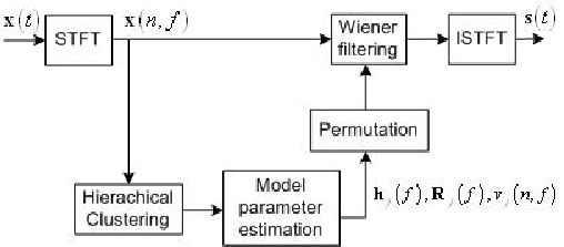
3.1 Initialization by hierarchical clustering
Preliminary experiments showed that the initialization of the model parameters greatly affects the separation performance resulting from the EM algorithm. In the following, we propose a hierarchical clustering-based initialization scheme inspired from the algorithm in [2].
This scheme relies on the assumption that the sound from each source comes from a certain region of space at each frequency , which is different for all sources. The vectors of mixture STFT coefficients are then likely to cluster around the direction of the associated mixing vector in the time frames where the th source is predominant.
In order to estimate these clusters, we first normalize the vectors of mixture STFT coefficients as
| (16) |
where denotes the phase of a complex number and the Euclidean norm. We then define the distance between two clusters and by the average distance between the associated normalized mixture STFT coefficients
| (17) |
In a given frequency bin, the vectors of mixture STFT coefficients on all time frames are first considered as clusters containing a single item. The distance between each pair of clusters is computed and the two clusters with the smallest distance are merged. This ”bottom up” process called linking is repeated until the number of clusters is smaller than a predetermined threshold . This threshold is usually much larger than the number of sources [2], so as to eliminate outliers. We finally choose the clusters with the largest number of samples. The initial mixing vector and spatial covariance matrix for each source are then computed as
| (18) | ||||
| (19) |
where . Note that, contrary to the algorithm in [2], we define the distance between clusters as the average distance between the normalized mixture STFT coefficients instead of the minimum distance between them. Besides, the mixing vector is computed from the phase-normalized mixture STFT coefficients instead of both phase and amplitute normalized coefficients . These modifications were found to provide better initial approximation of the mixing parameters in our experiments. We also tested random initialization and direction-of-arrival (DOA) based initialization, i.e. where the mixing vectors are derived from known source and microphone positions assuming no reverberation. Both schemes were found to result in slower convergence and poorer separation performance than the proposed scheme.
3.2 EM updates for the rank-1 convolutive model
The derivation of the EM parameter estimation algorithm for the rank-1 convolutive model is strongly inspired from the study in [13], which relies on the same model of spatial covariance matrices but on a distinct model of source variances. Similarly to [13], EM cannot be directly applied to the mixture model (1) since the estimated mixing vectors remain fixed to their initial value. This issue can be addressed by considering the noisy mixture model
| (20) |
where is the mixing matrix whose th column is the mixing vector , is the vector of source STFT coefficients and some additive zero-mean Gaussian noise. We denote by the diagonal covariance matrix of . Following [13], we assume that is stationary and spatially uncorrelated and denote by its time-invariant diagonal covariance matrix. This matrix is initialized to a small value related to the average accuracy of the mixing vector initialization procedure.
EM is separately derived for each frequency bin for the complete data that is the set of mixture and source STFT coefficients of all time frames. The details of one iteration are as follows. In the E-step, the Wiener filter and the conditional mean and covariance of the sources are computed as
| (21) | ||||
| (22) | ||||
| (23) | ||||
| (24) | ||||
| (25) |
where is the identity matrix and the diagonal matrix whose entries are given by its arguments. Conditional expectations of multichannel statistics are also computed by averaging over all time frames as
| (26) | ||||
| (27) | ||||
| (28) |
In the M-step, the source variances, the mixing matrix and the noise covariance are updated via
| (29) | ||||
| (30) | ||||
| (31) |
where projects a matrix onto its diagonal.
3.3 EM updates for the full-rank unconstrained model
The derivation of EM for the full-rank unconstrained model is much easier since the above issue does not arise. We hence stick with the exact mixture model (1), which can be seen as an advantage of full-rank vs. rank-1 models. EM is again separately derived for each frequency bin . Since the mixture can be recovered from the spatial images of all sources, the complete data reduces to , that is the set of STFT coefficients of the spatial images of all sources on all time frames. The details of one iteration are as follows. In the E-step, the Wiener filter and the conditional mean and covariance of the spatial image of the th source are computed as
| (32) | ||||
| (33) | ||||
| (34) |
where is defined in (4) and in (5). In the M-step, the variance and the spatial covariance of the th source are updated via
| (35) | ||||
| (36) |
where denotes the trace of a square matrix. Note that, strictly speaking, this algorithm is a generalized form of EM [17], since the M-step increases but does not maximize the likelihood of the complete data due to the interleaving of (35) and (36).
3.4 EM updates for the rank-1 anechoic model and the full-rank direct+diffuse model
The derivation of EM for the two remaining models is more complex since the M-step cannot be expressed in closed form. The complete data and the E-step for the rank-1 anechoic model and the full-rank direct+diffuse model are identical to those for the rank-1 convolutive model and the full-rank unconstrained model, respectively. The M-step, which consists of maximizing the likelihood of the complete data given their natural statistics computed in the E-step, could be addressed e.g. via a quasi-Newton technique or by sampling possible parameter values from a grid [12]. In the following, we do not attempt to derive the details of these algorithms since these two models appear to provide lower performance than the rank-1 convolutive model and the full-rank unconstrained model in a semi-blind context, as discussed in Section 4.2.
3.5 Permutation alignment
Since the parameters of the rank-1 convolutive model and the full-rank unconstrained model are estimated independently in each frequency bin , they should be ordered so as to correspond to the same source across all frequency bins. In order to solve this so-called permutation problem, we apply the DOA-based algorithm described in [18] for the rank-1 model. Given the geometry of the microphone array, this algorithm computes the DOAs of all sources and permutes the model parameters by clustering the estimated mixing vectors normalized as in (16).
Regarding the full-rank model, we first apply principal component analysis (PCA) to summarize the spatial covariance matrix of each source in each frequency bin by its first principal component that points to the direction of maximum variance. This vector is conceptually equivalent to the mixing vector of the rank-1 model. Thus, we can apply the same procedure to solve the permutation problem. Fig. 2 depicts the phase of the second entry of before and after solving the permutation for a real-world stereo recording of three female speech sources with room reverberation time ms, where has been normalized as in (16). This phase is unambiguously related to the source DOAs below 5 kHz [18]. Above that frequency, spatial aliasing [18] occurs. Nevertheless, we can see that the source order is globally aligned for most frequency bins after solving the permutation.

4 Experimental evaluation
We evaluate the above models and algorithms under three different experimental settings. Firstly, we compare all four models in a semi-blind setting so as to estimate an upper bound of their separation performance. Based on these results, we select two models for further study, namely the rank-1 convolutive model and the full-rank unconstrained model. Secondly, we evaluate these models in a blind setting over synthetic reverberant speech mixtures and compare them to state-of-the-art algorithms over the real-world speech mixtures of the 2008 Signal Separation Evaluation Compaign (SiSEC 2008) [4]. Finally, we assess the robustness of these two models to source movements in a semi-blind setting.
4.1 Common parameter settings and performance criteria
The common parameter setting for all experiments are summarized in Table 1. In order to evaluate the separation performance of the algorithms, we use the signal-to-distortion ratio (SDR), signal-to-interference ratio (SIR), signal-to-artifact ratio (SAR) and source image-to-spatial distortion ratio (ISR) criteria expressed in decibels (dB), as defined in [19]. These criteria account respectively for overall distortion of the target source, residual crosstalk from other sources, musical noise and spatial or filtering distortion of the target.
| Signal duration | 10 seconds |
|---|---|
| Number of channels | |
| Sampling rate | 16 kHz |
| Window type | sine window |
| STFT frame size | 2048 |
| STFT frame shift | 1024 |
| Propagation velocity | 334 m/s |
| Number of EM iterations | 10 |
| Cluster threshold |
4.2 Potential source separation performance of all models
The first experiment is devoted to the investigation of the potential source separation performance achievable by each model in a semi-blind context, i.e. assuming knowledge of the true spatial covariance matrices. We generated three stereo synthetic mixtures of three speech sources by convolving different sets of speech signals, i.e. male voices, female voices, and mixed male and female voices, with room impulse responses simulated via the source image method. The positions of the sources and the microphones are illustrated in Fig. 3. The distance from each source to the center of the microphone pair was 120 cm and the microphone spacing was 20 cm. The reverberation time was set to ms.

The true spatial covariance matrices of all sources were computed either from the positions of the sources and the microphones and other room parameters or from the mixing filters. More precisely, we used the equations in Sections 2.2, 2.3 and 2.4 for rank-1 models and the full-rank direct+diffuse model and ML estimation from the spatial images of the true sources for the full-rank unconstrained model. The source variances were then estimated from the mixture using the quasi-Newton technique in [6], for which an efficient initialization exists when the spatial covariance matrices are fixed. Binary masking and -norm minimization were also evaluated for comparison using the same mixing vectors as the rank-1 convolutive model with the reference software in [4]. The results are averaged over all sources and all set of mixtures and shown in Table 2.
| Covariance models | Number of spatial parameters | SDR | SIR | SAR | ISR |
|---|---|---|---|---|---|
| Rank-1 anechoic | 6 | 0.8 | 2.4 | 7.9 | 5.0 |
| Rank-1 convolutive | 3078 | 3.8 | 7.5 | 5.3 | 9.3 |
| Full-rank direct+diffuse | 8 | 3.2 | 6.9 | 5.4 | 7.9 |
| Full-rank unconstrained | 6156 | 5.6 | 10.7 | 7.3 | 11.0 |
| Binary masking | 3078 | 3.3 | 11.1 | 2.4 | 8.4 |
| -norm minimization | 3078 | 2.7 | 7.7 | 3.4 | 8.6 |
The rank-1 anechoic model has lowest performance because it only accounts for the direct path. By contrast, the full-rank unconstrained model has highest performance and improves the SDR by 1.8 dB, 2.3 dB, and 2.9 dB when compared to the rank-1 convolutive model, binary masking, and -norm minimization respectively. The full-rank direct+diffuse model results in a SDR decrease of 0.6 dB compared to the rank-1 convolutive model. This decrease appears surprisingly small when considering the fact that the former involves only 8 spatial parameters (6 distances , plus and ) instead of 3078 parameters (6 mixing coefficients per frequency bin) for the latter. Nevertheless, we focus on the two best models, namely the rank-1 convolutive model and the full-rank unconstrained model in subsequent experiments.
4.3 Blind source separation performance as a function of the reverberation time
The second experiment aims to investigate the blind source separation performance achieved via these two models and via binary masking and -norm minimization in different reverberant conditions. Synthetic speech mixtures were generated in the same as in the first experiment, except that the microphone spacing was changed to 5 cm and the distance from the sources to the microphones to 50 cm. The reverberation time was varied in the range from 50 to 500 ms. The resulting source separation performance in terms of SDR, SIR, SAR, and ISR is depicted in Fig. 4.

We observe that in a low reverberant environment, i.e. ms, the rank-1 convolutive model provides the best SDR and SAR. This is consistent with the fact that the direct part contains most of the energy received at the microphones, so that the rank-1 spatial covariance matrix provides similar modeling accuracy than the full-rank model with fewer parameters. However, in an environment with realistic reverberation time, i.e. ms, the full-rank unconstrained model outperforms both the rank-1 model and binary masking in terms of SDR and SAR and results in a SIR very close to that of binary masking. For instance, with ms, the SDR achieved via the full-rank unconstrained model is dB, dB and dB larger than that of the rank-1 convolutive model, binary masking, and -norm minimization respectively. These results confirm the effectiveness of our proposed model parameter estimation scheme and also show that full-rank spatial covariance matrices better approximate the mixing process in a reverberant room.
4.4 Blind source separation with the SiSEC 2008 test data
We conducted a third experiment to compare the proposed full-rank unconstrained model-based algorithm with state-of-the-art BSS algorithms submitted for evaluation to SiSEC 2008 over real-world mixtures of 3 or 4 speech sources. Two mixtures were recorded for each given number of sources, using either male or female speech signals. The room reverberation time was 250 ms and the microphone spacing 5 cm [4]. The average SDR achieved by each algorithm is listed in Table 3. The SDR figures of all algorithms except yours were taken from the website of SiSEC 200811 1 http://sisec2008.wiki.irisa.fr/tiki-index.php?page=Under-determined+speech+and+music+mixtures.
4.5 Investigation of the robustness to small source movements
Our last experiment aims to to examine the robustness of the rank-1 convolutive model and the full-rank unconstrained model to small source movements. We made several recordings of three speech sources , , in a meeting room with 250 ms reverberation time using omnidirectional microphones spaced by 5 cm. The distance from the sources to the microphones was 50 cm. For each recording, the spatial images of all sources were separately recorded and then added together to obtain a test mixture. After the first recording, we kept the same positions for and and successively moved by 5 and 10∘ both clock-wise and counter clock-wise resulting in 4 new positions of . We then applied the same procedure to while the positions of and remained identical to those in the first recording. Overall, we collected nine mixtures: one from the first recording, four mixtures with 5∘ movement of either or , and four mixtures with 10∘ movement of either or . We performed source separation in a semi-blind setting: the source spatial covariance matrices were estimated from the spatial images of all sources recorded in the first recording while the source variances were estimated from the nine mixtures using the same algorithm as in Section 4.2. The average SDR and SIR obtained for the first mixture and for the mixtures with 5∘ and 10∘ source movement are depicted in Fig. 6 and Fig. 6, respectively. This procedure simulates errors encountered by on-line source separation algorithms in moving source environments, where the source separation parameters learnt at a given time are not applicable anymore at a later time.


The separation performance of the rank-1 convolutive model degrades more than that of the full-rank unconstrained model both with 5∘ and 10∘ source rotation. For instance, the SDR drops by 0.6 dB for the full-rank unconstrained model based algorithm when a source moves by 5∘ while the corresponding drop for the rank-1 convolutive model equals 1 dB. This result can be explained when considering the fact that the full-rank model accounts for the spatial spread of each source as well as its spatial direction. Therefore, small source movements remaining in the range of the spatial spread do not affect much separation performance. This result indicates that, besides its numerous advantages presented in the previous experiments, this model could also offer a promising approach to the separation of moving sources due to its greater robustness to parameter estimation errors.
5 Conclusion and discussion
In this article, we presented a general probabilistic framework for convolutive source separation based on the notion of spatial covariance matrix. We proposed four specific models, including rank-1 models based on the narrowband approximation and full-rank models that overcome this approximation, and derived an efficient algorithm to estimate their parameters from the mixture. Experimental results indicate that the proposed full-rank unconstrained spatial covariance model better accounts for reverberation and therefore improves separation performance compared to rank-1 models and state-of-the-art algorithms in realistic reverberant environments.
Let us now mention several further research directions. Short-term work will be dedicated to the modeling and separation of diffuse and semi-diffuse sources or background noise via the full-rank unconstrained model. Contrary to the rank-1 model in [13] which involves an explicit spatially uncorrelated noise component, this model implicitly represents noise as any other source and can account for multiple noise sources as well as spatially correlated noises with various spatial spreads. A further goal is to complete the probabilistic framework by defining a prior distribution for the model parameters across all frequency bins so as to improve the robustness of parameter estimation with small amounts of data and to address the permutation problem in a probabilistically relevant fashion. Finally, a promising way to improve source separation performance is to combine the spatial covariance models investigated in this article with models of the source spectra such as Gaussian mixture models [11] or nonnegative matrix factorization [13].
References
- [1] O. Yılmaz and S. T. Rickard, “Blind separation of speech mixtures via time-frequency masking,” IEEE Trans. on Signal Processing, vol. 52, no. 7, pp. 1830–1847, July 2004.
- [2] S. Winter, W. Kellermann, H. Sawada, and S. Makino, “MAP-based underdetermined blind source separation of convolutive mixtures by hierarchical clustering and -norm minimization,” EURASIP Journal on Advances in Signal Processing, vol. 2007, 2007, article ID 24717.
- [3] P. Bofill, “Underdetermined blind separation of delayed sound sources in the frequency domain,” Neurocomputing, vol. 55, no. 3-4, pp. 627–641, 2003.
- [4] E. Vincent, S. Araki, and P. Bofill, “The 2008 signal separation evaluation campaign: A community-based approach to large-scale evaluation,” in Proc. Int. Conf. on Independent Component Analysis and Signal Separation (ICA), 2009, pp. 734–741.
- [5] E. Vincent, M. G. Jafari, S. A. Abdallah, M. D. Plumbley, and M. E. Davies, “Probabilistic modeling paradigms for audio source separation,” in Machine Audition: Principles, Algorithms and Systems, W. Wang, Ed. IGI Global, to appear.
- [6] N. Q. K. Duong, E. Vincent, and R. Gribonval, “Spatial covariance models for under-determined reverberant audio source separation,” in Proc. 2009 IEEE Workshop on Applications of Signal Processing to Audio and Acoustics (WASPAA), 2009, pp. 129–132.
- [7] C. Févotte and J.-F. Cardoso, “Maximum likelihood approach for blind audio source separation using time-frequency Gaussian models,” in Proc. 2005 IEEE Workshop on Applications of Signal Processing to Audio and Acoustics (WASPAA), 2005, pp. 78–81.
- [8] E. Vincent, S. Arberet, and R. Gribonval, “Underdetermined instantaneous audio source separation via local Gaussian modeling,” in Proc. Int. Conf. on Independent Component Analysis and Signal Separation (ICA), 2009, pp. 775–782.
- [9] A. P. Dempster, N. M. Laird, and B. D. Rubin, “Maximum likelihood from incomplete data via the algorithm,” Journal of the Royal Statistical Society. Series B, vol. 39, pp. 1–38, 1977.
- [10] J.-F. Cardoso, H. Snoussi, J. Delabrouille, and G. Patanchon, “Blind separation of noisy Gaussian stationary sources. Application to cosmic microwave background imaging,” in Proc. European Signal Processing Conference (EUSIPCO), vol. 1, 2002, pp. 561–564.
- [11] S. Arberet, A. Ozerov, R. Gribonval, and F. Bimbot, “Blind spectral-GMM estimation for underdetermined instantaneous audio source separation,” in Proc. Int. Conf. on Independent Component Analysis and Signal Separation (ICA), 2009, pp. 751–758.
- [12] Y. Izumi, N. Ono, and S. Sagayama, “Sparseness-based 2CH BSS using the EM algorithm in reverberant environment,” in Proc. 2007 IEEE Workshop on Applications of Signal Processing to Audio and Acoustics (WASPAA), 2007, pp. 147–150.
- [13] A. Ozerov and C. Févotte, “Multichannel nonnegative matrix factorization in convolutive mixtures for audio source separation,” IEEE Trans. on Audio, Speech and Language Processing, to appear.
- [14] H. Sawada, S. Araki, R. Mukai, and S. Makino, “Grouping separated frequency components by estimating propagation model parameters in frequency-domain blind source separation,” IEEE Trans. on Audio, Speech, and Language Processing, vol. 15, no. 5, pp. 1592–1604, July 2007.
- [15] T. Gustafsson, B. D. Rao, and M. Trivedi, “Source localization in reverberant environments: Modeling and statistical analysis,” IEEE Trans. on Speech and Audio Processing, vol. 11, pp. 791–803, Nov 2003.
- [16] H. Kuttruff, Room Acoustics, 4th ed. New York: Spon Press, 2000.
- [17] G. McLachlan and T. Krishnan, The EM algorithm and extensions. New York, NY: Wiley, 1997.
- [18] H. Sawada, S. Araki, R. Mukai, and S. Makino, “Solving the permutation problem of frequency-domain bss when spatial aliasing occurs with wide sensor spacing,” in Proc. 2006 IEEE Int. Conf. on Acoustics, Speech and Signal Processing (ICASSP), 2006, pp. 77–80.
- [19] E. Vincent, H. Sawada, P. Bofill, S. Makino, and J. Rosca, “First stereo audio source separation evaluation campaign: data, algorithms and results,” in Proc. Int. Conf. on Independent Component Analysis and Signal Separation (ICA), 2007, pp. 552–559.
- [20] M. Cobos and J. López, “Blind separation of underdetermined speech mixtures based on DOA segmentation,” IEEE Trans. on Audio, Speech, and Language Processing, submitted.
- [21] M. Mandel and D. Ellis, “ localization and separation using interaural level and phase cues,” in Proc. 2007 IEEE Workshop on Applications of Signal Processing to Audio and Acoustics (WASPAA), 2007, pp. 275–278.
- [22] R. Weiss and D. Ellis, “Speech separation using speaker-adapted eigenvoice speech models,” Computer Speech and Language, vol. 24, no. 1, pp. 16–20, Jan 2010.
- [23] S. Araki, T. Nakatani, H. Sawada, and S. Makino, “Stereo source separation and source counting with MAP estimation with Dirichlet prior considering spatial aliasing problem,” in Proc. Int. Conf. on Independent Component Analysis and Signal Separation (ICA), 2009, pp. 742–750.
- [24] Z. El Chami, D. T. Pham, C. Servière, and A. Guerin, “A new model based underdetermined source separation,” in Proc. Int. Workshop on Acoustic Echo and Noise Control (IWAENC), 2008.