Phase-field simulations of viscous fingering in shear-thinning fluids
Abstract
A phase-field model for the Hele-Shaw flow of non-Newtonian fluids is developed. It extends a previous model for Newtonian fluids to a wide range of shear-dependent fluids. The model is applied to perform simulations of viscous fingering in shear- thinning fluids, and it is found to be capable of describing the complete crossover from the Newtonian regime at low shear rate to the strongly shear-thinning regime at high shear rate. The width selection of a single steady-state finger is studied in detail for a 2-plateaux shear-thinning law (Carreau law) in both its weakly and strongly shear-thinning limits, and the results are related to previous analyses. In the strongly shear-thinning regime a rescaling is found for power-law (Ostwald-de-Waehle) fluids that allows for a direct comparison between simulations and experiments without any adjustable parameters, and good agreement is obtained.
I Introduction
The Saffman-Taylor instability occurs when a fluid is pushed by another one of lower viscosity in a confined geometry, such as porous media or a Hele-Shaw cell. It leads to the emergence of complex interfacial patterns whose shape is reminiscent of fingers. The study of this phenomenon [39, 35] has helped to establish much of our current knowledge on the self-organization of branched patterns [36, 6, 29]. Indeed, viscous fingering can be studied under well-controlled conditions in the laboratory using Hele-Shaw cells, where the flow is confined to a narrow gap between two parallel plates. In this geometry, the full flow can be well descibed by an effective two-dimensional problem, which greatly simplifies both theoretical analysis and numerical simulations.
For two Newtonian fluids of strongly different viscosities, our understanding is fairly complete. In a channel geometry, the instability of a flat interface and the subsequent evolution results in the formation of a single finger, the so-called Saffman-Taylor finger [39]. Its relative width with respect to the channel is selected by a subtle interplay between viscous dissipation and the surface tension of the interface, which acts as a singular perturbation. In a radial geometry, where the low-viscosity fluid is injected through a central inlet, fingers are not stable and exhibit repeated tip-splitting to form highly ramified patterns [36].
Much less is known about viscous fingering in non-Newtonian fluids. Numerous experiments have revealed that a wide variety of patterns can be formed, including finger patterns close to the ones found in Newtonian fluids with either narrowing or widening of the fingers, straight fingers in a radial geometry that do not exhibit tip splitting, and patterns that form angular branches and sharp tips, reminiscent of crack networks (for a review, see [34]).
It is clear that the selection of these patterns is governed by the nonlinearity of the fluid itself. More precisely, there is a complex interplay between the geometry of the finger, which determines the local flow pattern. The latter, in turn, modifies the properties of the fluids. In the particular case of shear-thinning fluids, the dependency of the fluid viscosity on the local shear rate, which strongly varies in the vicinity of a finger tip, can create an effect which is akin to an interfacial anisotropy. The latter is known both from experiments [5, 13, 38] and theory [28, 15] to profoundly affect pattern selection. Its presence suppresses tip-splitting and favors the emergence of dendritic patterns with sidebranches. The transition from branching fingers to dendrites observed in liquid crystals [10] can thus be explained, at least qualitatively [19, 22]. Furthermore, it is not surprising to see crack-like patterns in viscoelastic fluids [31], since a high shear around the tip pushes the fluid into the elastic regime.
For a more detailed and quantitative investigation of this relation between morphologies and the rheological properties of non-Newtonian fluids, precise numerical models would be very helpful. However, in mathematical terms, viscous fingering is normally formulated as a free boundary problem, which is quite difficult to handle numerically [40, 25, 17, 18]. To our best knowledge, simulations of non-Newtonian viscous fingering using such methods have remained limited to the case of shear-thinning fluids in the weakly shear-thinning limit [17, 18]. To overcome the difficulties due to moving interfaces, diffuse-interface and phase-field methods have become popular in many different fields [3, 9, 11, 23, 26]. In phase-field models, a continuous scalar field, the phase field, is introduced to distinguish between the two domains occupied by the two fluids. All properties of the fluids are interpolated through the diffuse interface, and the motion of the phase field is coupled to the equations of fluid dynamics. The original free boundary problem is obtained in the limit of vanishing interface thickness. While this approach introduces an additional scale (the interface thickness) into the problem, it removes the difficulties due to explicit interface tracking (non-uniform length change of the interfqce, topological changes). Therefore, its implementation is straightforward.
In this paper, we develop a phase-field model for Hele-Shaw flow in a wide class of fluids with a shear-dependent viscosity, by combining a phase-field model for Newtonian viscous fingering previously developed by one of us [20, 21] with a rigorous procedure for obtaining a generalized Darcy’s law for non-Newtonian fluids developed by Fast et al. [17]. The model is implemented using a finite-difference scheme in conjunction with a standard SOR solver for the pressure equation. We validate our model and implementation by a detailed comparison of the Newtonian case to the known sharp-interface solution. This allows us to estimate the errors that are due to the finite interface thickness and the discretization.
Although our model is capable of describing two non-Newtonian fluids with general shear-dependent viscosity laws, we limit ourselves to shear-thinning fluids pushed by a Newtonian fluid. Indeed, this is the setting where the most precise knowledge on pattern selection in non-Newtonian fluids is already available, and therefore it constitutes an excellent testing ground for our model. Data on the shape and width of steady-state fingers for shear-thinning fluids with a well-characterized viscosity law have been published [32, 33]. Furthermore, these data are in good agreement with theoretical studies that predict a narrowing of the steady-state fingers with respect to the Newtonian case [37, 2].
We perform simulations for two different viscosity laws, namely, a two-plateau law used in the simulations of Refs. [17, 18], and the one-plateau law which describes well, for the experimental flow regime, the fluids used in experiments of Refs. [32, 33]. We study the effect of the shear thinning on the selection of the finger width, and demonstrate that our model is able to cover the complete crossover from Newtonian behavior at low speed to strong shear-thinning at high speeds. More precisely, the selection of the finger width can be understood in terms of two dimensionless parameters: the Weissenberg number , which characterizes the strength of the shear-thinning effect, and a dimensionless surface tension . In general, the finger width depends on both parameters. However, it turns out that in the regime covered by the experiments [32, 33], the viscosity law can be well described by a simple power law. In this case, the finger width depends only on a single parameter, which is a function of , and the exponent of the viscosity law. In this regime, our simulations are in good agreement with the experimental data of Refs. [32, 33], which demonstrates the capability of our model to yield quantitatively accurate results.
II Model
II.1 Sharp-interface equations
We consider two incompressible, immiscible fluids (labeled 1 and 2) in a Hele-Shaw cell of width (-direction), length (-direction) and gap (-direction, ). The less viscous fluid 2 is injected at one end of the cell with a fixed flow rate , causing outflow of fluid 1 at the other end of the cell with a velocity . The interface between the two fluids has a positive surface tension . Both fluids, may have a non-Newtonian shear viscosity that depends on the local shear rate , , where is a characteristic relaxation time of fluid ; we furthermore suppose that both viscosity laws have well-defined Newtonian limits when , which we will denote by .
As usual in a Hele-Shaw cell at low velocities (where inertia can be neglected), the scale separation between the gap and the channel width makes it possible to simplify the full three-dimensional flow problem by a long-wave approximation. The resulting two-dimensional problem is stated, for each fluid, in terms of the pressure field (which is constant across the gap) and the gap-averaged in-plane velocity . These two-dimensional velocity fields remain incompressible,
| (1) |
Furthermore, for Newtonian fluids, the local averaged velocity is proportional to the local in-plane pressure gradient, a relationship known as Darcy’s law. For non-Newtonian fluids, the relationship between and becomes non-linear, but can formally still be written as a generalized Darcy’s law,
| (2) |
where is an effective viscosity, which can be related to the original shear-dependent viscosity for a large class of non-Newtonian fluids following the procedure developed by Fast et al. [17], which is summarized and presented using the notations of the present work in Appendix A. We have included the constants , and in the argument of the effective viscosity to emphasize that this argument is indeed a dimensionless shear. The characteristic local shear rate can be estimated by the ratio of the gap-averaged velocity and the cell gap ; the order of magnitude of the velocity, in turn, is given by (see Appendix A for details). Note that we have chosen to express the viscosity as a function of the pressure gradient (and not of the velocity as in [37, 2, 32, 33]) in order to formulate the model in terms of the interface geometry and the pressure field only. One should note that for a vanishing shear rate (), we have , and Eq. (2) reduces to the standard Darcy’s law.
Since we are considering two fluid regions separated by an interface, we have to specify the boundary conditions at the interface:
| (3) | |||||
| (4) |
where is the interface curvature (in the plane of flow), is the surface tension and is the unit vector normal to the interface pointing into fluid 1. Equation (3) is simply the Laplace law, where the curvature of the meniscus between the plates has been omitted under the assumption that it is constant. Eq. 4 simply assures the impenetrability of the two fluids.
In order to make this formulation more directly amenable to the construction of a phase-field model, we rewrite the above equations in terms of a single set of fields and material properties [14],
| (5) | |||||
| (6) | |||||
| (7) |
where and are the characteristic functions of the domains occupied by the two fluids (that is, if the point is occupied by fluid , and otherwise). We thus reduce Eqs. (2, 3 and 1) to just two:
| (8) |
| (9) |
where is a surface delta function (that is, a Dirac delta function located on the sharp interface separating the two fluid domains [14]). Now all fields, material properties and equations must be understood in the sense of mathematical distributions. As such, these equations, apart from their obvious limits at each side of the interface, are to be understood when integrated across the interface. In particular, integrating the normal projection of the velocity times the effective viscosity in Eq. (8) across the interface gives the Laplace pressure drop of Equation (3). Similarly, the condition of zero divergence of Equation (9) relates the normal and tangential components of the fluid velocity. The condition of incompressibility, when applied on the very interface, translates into impenetrability of the two fluids.
II.2 Phase-field model
In this section, we present the phase field approach to this problem. We first give a brief description of the phase field (denoted by ) and show how using it instead of the indicator functions, the flow equations (8) and (9) are modified. Then we present the evolution equation for the phase field and give a rationale for its construction. Finally, we comment briefly on how the phase-field model is an approximation of the sharp-interface model.
The idea underlying the phase-field model is to introduce an additional field () that indicates in which phase (here, in which fluid) the system is at a given space point. For the sake of simplicity and without any loss of generality, we consider that in fluid 1 (resp. 2) , . In addition, when crossing the interface the phase field exhibits a smooth front (kink) of finite width. In this general framework, the indicator functions and the function are approximated by
| (10) | |||||
| (11) | |||||
| (12) |
Then, replacing and by their smoothed expressions, the effective viscosity of Eq. (7) becomes
| (13) |
Note that, as in Eq. (70, formally is a function of because is a function of . Darcy’s law becomes
| (14) |
where is the curvature of the interface computed using the standard expressions
| (15) |
Note that is now defined in the entire space; is the local normal to the isosurface. Equation (9) for the incompressibility of the flow is not modified by the introduction of the phase field. Now, the flow problem is completely written in terms of the phase field.
To complete the model, we have to introduce an evolution equation for the phase field. This evolution equation should have for solution a smooth interface that is advected by the flow To this purpose, we use the equation presented in [20] and extended with success in [7, 8] to the case of vesicles:
| (16) |
with the oposite of the derivative of the double well potential , a relaxation time, and a small parameter that determines the width of the interface. In order to give a clear view of the equation, we first consider an oversimplified version of it with neither the flow nor the curvature term, in a one-dimensional space. The stationary solutions of this equation are either the uniform solutions or a front between a region where and a region where :
| (17) |
Here, the signification of appears clearly: it is the width of the interface. Now let us consider this equation (still without flow and without the curvature term) in two dimensions. Using a perturbation method, one can show that a weakly curved interface (radius of curvature ) between and is moving with a normal velocity proportional to , the curvature of the interface. While this behaviour is expected in the case of phase transitions with non-conserved order parameters, here it is unphysical. In order to suppress this phenomenon, following [20] we add the curvature term which at dominant order is the exact opposite of the term induced by the Laplacian when considering a curved interface. Indeed, it can be shown that up to the third order in , the term is equal to the unidimensional Laplacian computed along the axis normal to the interface. Hence, using (with the distance from the center of the interface), the right-hand side of Eq. (16), i.e. the driving force leading to unwanted interface movement, is equal to zero up to that third order.
Finally, adding the term makes the interface to be advected by the flow. Therefore, the dynamics of the phase field can be separated into two parts: a passive part that corresponds to the advection due to the flow and an active part that aims at restoring the hyperpolic tangent profile through the interface but does not bring any noticeable dynamics to the interface. With this principle in mind, it is clear that the relaxation time of the phase field must be fast enough so that the advection does not affect significantly the equilibrium profile. The particular choice of is discussed later.
Now, that model equations have been written down, we want to stress that while the distribution formulation of the viscous fingering problem is just another way of writing down the same sharp-interface equations, the phase-field model is only an approximation to them. To be more specific, the phase field model introduces an additional length scale , the interface thickness, which is a model parameter supposed to be small. To understand its meaning and the relationship between the phase-field approach and the sharp interface model, one can use the technique of matched asymptotics. Different asymptotic expansions of the phase field equations in powers of valid in the bulk phases and through the interface, respectively, are written down. Then, matching them order by order, at dominant order in the original sharp interface-problem is retrieved, which indicates that the results of the phase-field model converge toward the solution of the original problem when (the so called sharp-interface limit). In other words, the model is at least asymptotically correct.
However, in numerical simulations, the value of should be significantly larger than the space discetization and must remain finite. Therefore, to be able to retrieve quantitatively correct results, one needs to control the spurious effects introduced by the finite interface thickness and the convergence of the model toward the sharp-interface limit. This can be done by considering the next order in in the matching procedure [27, 1, 20, 16]. Then, new -dependent terms are added to the sharp interface equations (this next order in the expansion is called the thin-interface limit). They actually signal the departure from the limit and are the effect of the presence of the extra length scale. Physically, one expects their importance to depend on the ratio of to the smallest genuine length scale present in the original sharp-interface model. This hypothesis can then be checked by simulations with decreasig values of that ratio [27, 21, 16].
Here, we have written our model so that, in the case of Newtonian fluids, it is mathematically equivalent to the one presented in [20]. The reason for this is that contrary to other phase field models [30, 24] for viscous fingering, the asymptotic expansions of this model have been established [20] and the numerical convergence has been checked by considering situations where the sharp interface solution is well known [21]. Therefore, we are confident that unexpected finite interface thickness effects could only arise in our simulations in conjunction with the new feature here: the non-Newtonian character of the more viscous fluid.
II.3 Dimensionless equations
In order to nondimensionalize our equations, we first look at the relevant physical scales present in the flow, and then use the same scales to nondimensionalize the phase-field equation. Non-dimensionalized quantities will be denoted by a tilde. In a first step, we define dimensionless effective viscosity functions by dividing the effective viscosity laws of the two fluids by their zero-shear limit values ,
| (18) |
Next, since in a phase-field model there is a generalized effective viscosity valid throughout the system [Eq. (13)] which interpolates between the effective viscosities of each fluid, we need to choose a single viscosity scale. This choice has to be adapted to the physical situation that is investigated. Here, we are mainly interested in the setting used in most experiments, where the more viscous fluid 1 is a shear-thinning liquid and the less viscous fluid 2 is air, that is, a Newtonian fluid of very low viscosity. Therefore, in the following we will nondimensionalize the effective viscosity by the zero-shear viscosity of fluid 1, . Since fluid 2 is Newtonian, we have .
With the above choices, the nondimensionalized effective viscosity function becomes
| (19) |
where is the ratio of the two zero-shear viscosities,
| (20) |
This ratio can be simply related to the quantity
| (21) |
the so-called viscosity contrast (at zero shear), also widely used in the literature [40, 20].
We furthermore measure velocity in units of the outflow velocity and lengths in units of the channel width . The natural scale for the pressure gradient that arises from the Newtonian limit of Darcy’s law is . This yields the new dimensionless quantities
| (22) | |||
| (23) | |||
| (24) |
Under this change of variables, the arguments of the dimensionless effective viscosity function given by Eqs. (18,19) become
| (25) |
where the Weissenberg number is defined by
| (26) |
In the remainder of this paper (except for Appendix A), we will work in these new dimensionless variables and drop the tildes for simplicity.
The incompressibility condition remains formally the same, and the dimensionless version of Darcy’s law reads
| (27) |
where
| (28) |
is a dimensionless surface tension. In summary, the flow equations contain three dimensionless parameters: the dimensionless surface tension , the Weissenberg number , and the viscosity ratio . A more detailed discussion of these parameters and their role in the finger selection process is deferred to Sec. II.6 below.
To complete the set of dimensionless equations, we apply the same scaling to Eq. (16) for the phase field. We obtain
| (29) |
and identify the dimensionless interface thickness , the ratio of the interface thickness to the channel width. In order to reduce the number of purely computational parameters, we choose . Indeed, is the time it takes a flow of the magnitude of the base flow to cover one interface thickness , and the extra small factor ensures that the phase field relaxation is one order in faster than the forcing by the flow. We finally get
| (30) |
II.4 Incompressibility and boundary conditions
In the simulations, Eq. (30) for the phase field and the fluid flow equations need to be solved simultaneously. The fluid flow part, in turn, implies solving Eq. (27) taking into account the incompressibility condition, Eq. (9). There are several ways to implement incompressibility.
One possibility is to take the curl of Eq. (27), which eliminates the pressure field in the Newtonian case. Incompressibility is equivalent to the requirement that the flow is potential, that is, the velocity field can be written as derivatives of the stream function. The curl of Eq. (27) yields a Poisson equation for the stream function. This strategy leads exactly to the model of Ref. [20] for Newtonian fluids, as desired.
However, for non-Newtonian rheologies, the dependence of the effective viscosity on implies that the pressure cannot be eliminated in this straightforward manner any more. Therefore, we use here a velocity-pressure formulation: We take the divergence of Eq. (27) and use the incompressibility condition, which yields
| (31) |
For a given configuration of the phase field , Eq. (31) together with appropriate boundary conditions (discussed below) completely specifies the pressure field . In the Newtoninan limit where the effective viscosity is pressure-independent, this equation is a Poisson equation for the pressure inside the interfacial regions where the phase field varies, and reduces to the Laplace equation in each bulk domain. In the non-Newtonian case, the source term is present also in the bulk, and an iterative Poisson solver must be used to obtain the pressure field for the given configuration of the phase field at each timestep. Then, the original Eq. (27) immediately yields the velocity field . This is then used in the next time step to advect the phase-field , as prescribed by Eq. (30). More details about the numerical procedure are given in Appendix B.
Furthermore, boundary conditions for the phase and pressure fields are required at the edges of the channel. For simplicity, we will assume that if an interface crosses any of the boundaries, it will do so at a 90∘ angle, which implies that the derivatives of the phase-field normal to the boundaries are zero (reflecting boundary conditions):
| (32) | |||||
| (33) |
Since the lateral walls are sealed and hence , we also have
| (34) |
The only non-trivial boundary conditions are the pressure boundary conditions at the inlet and the outlet, where either the pressure or its gradient have to be prescribed. Since we have considered a flow with a fixed overall flow rate, we should prescribe the pressure gradient.
At the outlet, only fluid 1 is present. If the interface remains far enough from the outlet, the pressure is simply a constant along the entire outlet, and the pressure gradient is directed along the direction. Since, at the outlet, the dimensionless velocity is equal to (corresponding to a uniform flow with velocity along the direction), the Darcy law (eq. 27) implies that the pressure gradient is the solution of the equation
| (35) |
where the velocity enters the equation through the Weissenberg number. This equation can be solved numerically in a straightforward way. In our simulations, we start with an initial guess for the pressure gradient, which is then updated at each time step with the value found by the pressure solver in the vicinity of the outlet. This procedure rapidly converges to the fixed point which is the solution of Eq. (35).
As for the inlet, we consider the case where both fluids are present. For a well-developed steady-state Saffman-Taylor finger, the sides of the finger are parallel to the channel walls up to a correction that decays exponentially with the distance from the finger tip. Therefore, if a sufficiently long portion of the finger is inside the simulation box, the interfaces that cross the inlet can be considered flat and normal to the boundary, and the fluid velocity along the direction is zero in both fluids. Therefore, there is no pressure gradient along the direction, which of course implies that the pressure gradient is directed along , and constant along the inlet.
In contrast, the fluid velocity varies along the inlet, since the viscosity does change when crossing the interface. However, its integral along , , which represents the net inward flow, must be equal to unity, since the flow is incompressible and the fluid exits the outlet at a rate of unity in our dimensionless variables. Integrating the component of Eq. (27) along the inlet, we thus obtain
| (36) |
which constitutes a closed equation for the desired value of at the inlet.
II.5 Simulation procedure
In our numerical studies, our main focus is on steady-state fingers. Although we could start each simulation with a weakly perturbed flat interface and let it follow its natural dynamics until a steady finger stabilizes, this is not the most efficient procedure for parametric studies of the finger width as a function of and . Therefore, we instead first calculated an initial finger profile for values of the control parameters where convergence can be easily achieved, and then use the resulting steady-state pressure and phase fields as initial condition for a run with slightly different control parameters. Increasing or decreasing and/or in small steps, we are thus able to follow the steady-state solution branches over a substantial parameter range.
When performing the first computation for a given viscosity law, we set the initial interface profile to a semi-elliptic bubble (of width and length ) growing from the inlet of the channel. The initial configuration of the phase field is a hyperbolic tangent profile in the elliptic coordinates, and its zero contour is located at the elliptic bubble interface. The simulations are performed in a channel with a length of . The bubble increases in size and depelops into an elongated finger. When it reaches a reference position (typically, located at twice the channel width from the inlet), the whole domain is translated backward by one grid spacing (in other words, the finger is pulled back by one grid point). The velocity of the finger is computed by measuring the time between two successive pullbacks. The finger width is measured at the entrance of the channel when a pullback occurs. We consider the steady reached when both tip velocity and finger width vary less than a fixed value (here chosen to be , to be compared with a typical tip velocity of 2 and a typical finger width of 0.5) between two pullbacks.
Values of of the order of yield a rapid convergence to a steady-state finger, both for Newtonian and non-Newtonian fluids. For the latter, the convergence is more difficult to obtain because of the nonlinearities in the viscosity laws. Typically, we calculate the first finger with a low value of the Weissenberg number for which these nonlinearities are small; is then increased progressively up to the desired value. In this way, values up to can be treated, for which the pressure solver would have otherwise not converged. As for , the values we are able to attain are limited both from below and from above. For small values of , results become sensitive to the discretization and the interface thickness, as will be detailed below. For large values of , the finger width becomes close to unity, and the tail of the phase-field profile starts to interact with the sidewalls.
The solutions found in our simulations are single fingers propagating at constant velocity along the channel. We consider fingers symmetric with respect to the channel mid-line . This allows us to reduce the computation time by limiting the numerical domain to half the channel: ). The validity of this procedure was checked by occasinally performing computations in the full domain: fingers started with an axis of symmetry shifted away from the mid-line always relax towards the center of the channel in finite time. We have also checked that increasing the length of our simulation domain (changing the aspect ratio ) does not change the results. Indeed, in our typical steady-state configuration, the back of the finger is cut off at twice the channel width behind the tip, where its flanks are almost flat and fluid 1 is almost at rest. Furthermore, the pressure field becomes almost linear far ahead of the tip, and a distance of three times the channel width is enough to resolve all non-trivial features of the velocity and pressure fields.
In our simulations we let the finger extend inside the channel until the tip crosses a reference position along the axis. When this happens, the time step is truncated so that the finger tip advances exactly to the pullback coordinate; the whole field is then pulled one grid step backward. The velocity of the finger is obtained by computing the average velocity between two successive pullbacks. The finger width is measured at the entrance of the channel when a pullback occurs. The stationary state is declared to be achieved when both tip velocity and finger width vary less than a fixed value, here chosen to be .
The computation time necessary to achieve the stationary state for a given value can be significantly reduced when the run is initialized with a finger profile close enough to the converged state. Hence we applied the following procedure to obtain selection curves in the Newtonian and the shear thinning cases:
For the first computation of the set, the phase field is initialized with a semi-elliptic bubble growing from the inlet side of the channel. The small radius spans over half the width of the channel and the big radius is arbitrarily chosen to be the channel width in the longitudinal direction. The phase field obeys a hypertangent profile in elliptic coordinates. A moderate parameter of is chosen to compute the first finger profile. The parameter is then varied towards zero and towards infinity to move along the selection curve. Each computation is initialized with the finger profile at numerical convergence. Attainable values are both limited in the small and large limits. In the former case, the interface thickness needs to be reduced, and thus the grid refined, in order to retain the relevant selection mechanism. In the latter case, the stationary solution can be destroyed when the phase field is too close to the boundaries. In the non-Newtonian case the first step is more difficult because of the nonlinearities in the viscosity. We do not impose the correct pressure condition at the outlet, but rather let it relax as time is stepped forward.
II.6 Control parameters and finger selection
The independent parameters that appear in our equations are the zero-shear viscosity ratio (constant for a given pair of fluids), the Weissenberg number , which controls the intensity of the shear-thinning effect, and the dimensionless surface tension . It is noteworthy that in experiments performed with a single Hele-Shaw cell of fixed width and gap spacing, both and increase linearly with [see Eqs. (26),(28)], which is the only parameter that can be externally controlled. The full two-dimensional parameter space can hence only be explored in experiments by varying the channel geometry as well as . In contrast, in the simulations it is easy to vary these two parameters independently, and to determine the selected finger width. However, it is useful to take some additional considerations into account.
It is known that two main ingredients determine the finger width: the dimensionless surface tension and the anisotropy of the interface or the medium. In shear-thinning fluids an effective anisotropy arises from the fact that the in-plane velocity and thus the shear are maximal at the tip, and decay when going to the sides of the finger. As a consequence, the viscosity and hence the mobility in Darcy’s law vary along the interface. Thus, the strength and nature of this effective anisotropy are essentially controlled by the Weissenberg number and the functional form of the viscosity law.
Let us now turn to the dimensionless surface tension. For Newtonain fluids, it was shown [35] that the selection of the finger width is determined by a single dimensionless parameter , which represents the ratio of stabilizing (capillary) to destabilizing (viscous) forces. The latter are proportional to the finger speed and the difference of the two viscosities (see e.g. Ref. [40]). In shear-thinning fluids, the relevant viscosity is the one in the vicinity of the tip, and the correct definition of the parameter is
| (37) |
Using the definition of and the fact that mass conservation for an incompressibe fluid enforces for a steady-state finger of relative width , we find the following relation between and :
| (38) |
Ideally, we would like to explore the parameter space along lines of constant in order to track only the influence of the effective anisotropy (the selection parameter of the isotropic Saffman-Taylor problem is then constant). However, is difficult to control directly in our simulations: the effective viscosity at the tip, which is needed to calculate , depends on the finger speed, which is itself the result of the selection to be investigated. Therefore, we explore the width selection by varying either at fixed , or at fixed , and calulate a posteriori using the tip speed and pressure gradient extracted from the simulations. Note that this procedure is perfectly analogous to the one followed in experiments: the viscosity at the tip is estimated a posteriori using the measured finger speed [32, 33]. Keeping constant is more involved, and would require some iterative trial and error procedure, which is perfectly feasible but cumbersome.
A last point that deserves brief mention is the viscosity ratio . In the case of air pushing a viscous fluid, is extremely small, so that the viscosity of the air can be neglected altogether. In our numerical formulation, however, it is difficult to simulate very small values of , because Eq. (31) then has extremely different numerical stiffness in the two bulk domains, which makes the convergence of the pressure solver delicate. In our simulations, we have typically used values of ranging from to , which are large enough to guarantee a robust and efficient solution of Eq. (31). One could think that these are small enough to neglect in the denominator of Eq. (38). However, as will be seen below, for a viscosity law without lower bound (such as a power-law), the viscosity of the shear-thinning fluid will become comparable to or even smaller than that of the pushing Newtonian fluid even for , for sufficiently high Weissenberg numbers. In the latter case, the fingering instability disappears altogether. We insist that this is an entirely physical effect that should be experimentally observable in fluid couples of not too different viscosities.
III Results
III.1 Newtonian fluid
In order to test our model formulation and its numerical implementation, we start by performing simulations in Newtonian fluids. The simulations converge without difficulty to a steady-state finger solution. In Fig. 1 we display a comparison between a typical finger shape extracted from our simulations and the analytical solution of Saffman and Taylor [39],
| (39) |
After fitting , the agreement between the computed and analytical curve is good. There are some small discrepancies close to the finger tip that are to be expected, since the solution given by Eq. (39) does not contain the effect of surface tension. That the latter is correctly incorporated into our model is proven by the results shown in Fig. 2, where we display the selection curve for the finger width at fixed values of and as a function of the dimensionless combination of parameters used in the classical work of Mc Lean and Saffman [35], which we compare to. The agreement is excellent, except for very small values of . This constitutes an extremely sensitive test for our model since the finger width is selected by the surface tension (via the selection parameter ) through a singular perturbation mechanism.


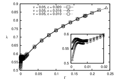

In Fig. 3 we replot the selection curve directly as a function of , to make the deviations from the analytical prediction for small values of most apparent. These deviations take place for ; Below that value, the decrease of the finger width with the dimensionless surface tension to the predicted limit value of for (note that for a Newtonian fluid, is just proportional to ) is interrupted by a small “bump”. Two effects limit the precision of our results. First, it is expected that at low values of smaller values of are needed to obtain properly resolved results. The reason is that the wavelength of the marginally stable mode of the linear Saffman-Taylor instability scales as . As in any phase-field model, the correct interface dynamics can only be guaranteed a priori when remains smaller than this value (i.e., well into the thin-interface limit). Deviations from the sharp-interface solution are thus simply a sign of insufficient resolution of the relevant length scale by the phase field. The second effect is purely numerical: when is decreased the surface tension effect becomes numerically small. More precisely, the pressure gradient accross the interface created by the Laplace pressure becomes smaller and smaller with respect to the global driving pressure gradient. Therefore, discretization errors can become significant. In particular, the anisotropy induced by the discretization on a regular lattice can have a strong effect on the solution. This is especially critical, since it is known that even a small amount of interfacial anisotropy dramatically modifies the selection mechanism [28, 15].
In Fig. 3, we test the importance of these two effects. Whereas a reduction in at fixed resolution (that is, constant ) reduces the height of the “bump”, the change of sign in slope occurs always at similar values of . In contrast, if the mesh is refined at fixed , the change in slope is shifted towards smaller values of . This indicates that the numerical discretization error is the dominant effect. Since a further decrease in the grid spacing would require a much larger computation time, we have limited our study to the regime of intermediate values of .
Incidentally, an observation we find worth reporting is that of symmetrical pulsating fingers (i.e. time-periodic solutions with oscillating width and tip velocity), albeit in a parameter region where the numerical convergence is not guaranteed ( slightly below ). These oscillations disappeared after further grid refinement. This is consistent with the picture [6] according to which the threshold in the logarithm of the amplitude of the noise (here numerical and related to the grid) needed to nonlinearly destabilise a Saffman-Taylor finger decays linearly with , , .
III.2 Shear-thinning fluids
To study the effect of shear thinning, we first need to specify the viscosity law. As an example, we take a two-plateau Carreau fluid, whose viscosity obeys the equation
| (40) |
Besides the already introduced relaxation time and zero-shear viscosity , this law has an inifinite-shear asymptote at the value and an exponent . It describes three regimes: two Newtonian plateaux at zero and infinite shear, where the viscosity is independent of the shear rate, and a shear-thinning region in between. The ratio of the heights of the two plateaux can be defined, , whereas the slope in the shear-thinning regime is determined by both and .
In the following, we address two limiting cases of this general law: the weakly ( not too small, see below for a more precise statement) and the strongly () shear-thinning regimes. No analytic expression for the corresponding effective viscosity (to be used in Darcy’s law) is known in either limit.
III.2.1 Weakly shear-thinning fluids
We first consider the weakly shear-thinning case and set in Eq. (40) to make contact with Ref. [17]. It was shown there that the resulting law translates into an effective viscosity in Darcy’s law as long as , so for practical purposes that sets the minimal value of which we mean when we refer to the “weakly” shear-thinning case. However, no closed analytical expression for this effective viscosity seemed possible, but the same functional dependence as the viscosity law Eq. (40) with turned out [17] to provide an excellent approximation for it:
| (41) |
where we recall that the Weissenberg number is given by . We therefore use this law in the remainder of this section.
The value corresponds to a Newtonian fluid; when decreases, the viscosity variations become steeper. We recall that there are now two independent parameters that control the finger selection (on top of ): , as in Newtonian fluids, and , which measures the strength of the shear-thinning effect. We begin by investigating the role of .
Let us first illustrate the origin of the effective anisotropy effect for shear-thinning fluids by display maps of the local effective viscosity function , Fig. 4, in various flow regimes, i.e., for various ranges of values. We find it clearer to begin with a description of the velocity field, since it relates directly to the local viscosity through the shear rate, which is proportional to the gap-averaged velocity. Far ahead of the finger, the local velocity is as in the outlet. The speed increases when the finger is approached, since the finger tip speed, is larger. Indeed, this is the maximal speed in the system. Further upstream (along the finger flanks) the speed of fluid 1 decreases to its limiting value, which can be computed using Eq. 36 and is of the order of . For (inviscid pushing fluid) the limiting value is 0.


With this picture in mind, the shear-thinning phenomenon upon increasing should be clearer. For , we remain in the low-shear Newtonian plateau of the viscosity, which is hence homogeneous. As (), the speed at the finger tip enters the shear-thinning regime, so the effective viscosity exhibits a well-marked minimum there. Furthermore, it increases towards its Newtonian limit along the finger sides, and it also increases ahead of the finger and towards the outlet. This picture remains valid when increases further, with the only difference that the region where the Newtonian regime is reached is sent further upstream along the finger flanks. Eventually, for (), a third regime appears: The fluid at the finger tip enters the high-shear-rate plateau of the viscosity law, so the viscosity becomes homogeneous in a growing region close to the tip, although it remains its absoute minimum in space. Soon the outlet is taken by this homogeneous-viscosity region, since the speed there is typically just a factor 2 smaller than at the tip. However this is not the case of the finger flanks, where the fluid speed decreases much more upstream, so they remain a shear-thinning zone, provided is small enough. This shear-thinning zone expands and moves upstream as is furhter increased; if is kept constant, it will eventually reach the inlet, and if is even increased further, the whole shear-thinning zone will “pass” through the inlet until the spot reaches the high-shear plateau and the viscosity becomes homogeneous again everywhere (but now lower). This happens at for , regardless of the finger length simulated.

In Fig. 5, we show the selected finger width as a function of at fixed for various values of and . For small values of , the shear-thinning fluid is in the high viscosity plateau and the finger width is almost constant. When is increased and approaches unity, the finger width decreases. The curve goes through a minimum, after which the finger width increases with until it becomes constant again when the shear-thinning fluid enters the second plateau.
The finger width for given and is larger at than at . This is a consequence of the relation between the control parameter and the tip selection parameter already discussed in Sec. II.6: the control parameter is defined with the viscosity of the first Newtonian plateau. However, at high shear rates, the fluid around the tip is in the second plateau, and therefore the width selection is governed by the corresponding value of the viscosity. Neglecting the viscosity of the Newtonian fluid (that is, setting ), we obtain at high Weissenberg numbers the simple relation , whereas for low , . Since , larger fingers are selected for high . This argument is corroborated by the two curves for , and , , which tend to the same finger width at high (Fig. 5). Indeed, they have the same value of in that regime.
A noteworthy feature of Fig. 5 is that all the curves for exhibit finger widths that are lower than , which is the smallest value that can be achieved in Newtonian fluids. This narrowing is due to the effective anisotropy induced by the shear-thinning effect in the medium, as can be appreciated from the viscosity maps in Fig. 4: the region of lower viscosity right in front of the finger tip facilitates the advance of the interface in the center of the channel. It is thus not surprising that the lowest values of the finger width are reached for , where the variations of the viscosity close to the tip are the strongest. Furthermore, this effect increases with decreasing , as can be seen by comparing the three curves obtained at in Fig. 5. They coincide at small values since the first Newtonian plateau is the same for all the curves. When approaches unity, the finger width decreases, with smaller giving rise to narrower fingers. This is to be expected since a smaller implies stronger variations of the viscosity with the shear rate, and thus a stronger effective anisotropy. At , the curves cross. Now lower values of give rise to wider fingers. This is due to the global decrease in viscosity in the shear-thinning fluid already discussed above, together with the weakening of the shear-thinning effect around the tip when the fluid enters the second Newtonian plateau.
From the preceding discussion, it is clear that for the effective viscosity law given by Eq. 41 the strongest shear-thinning effect occurs for . Therefore, next, we fix and study the selected finger width as a function of for various values of . As discussed previously, in order to display the results in a meaningful way, finger widths need to be plotted as a function of , which can be calculated a posteriori using Eq. (37). Figure 6 displays three selection curves for and , compared with the corresponding Newtonian curve at . The curve for is very close to the Newtonian one; with decreasing values of , the selected finger width decreases at fixed , which is consistent with the picture of an effective anisotropy increasing with . It should also be noted that, as for the Newtonian fluid, a “bump” occurs in the selection curve due to discretization effects; however, for strongly shear-thinning fluids there clearly exists a range of for which the solution is not affected by numerical artifacts, and for which stationary fingers display a width , which would be impossible for a Newtonian fluid.

III.2.2 Strongly shear-thinning fluid
We now turn to the case in which the shear-thinning effect is strong, that is, the infinite-shear viscosity can be neglected in front of the zero-shear viscosity, or . Then, the high-shear plateau disappears, and the two-plateau law of Eq. (40) becomes a one-plateau Carreau law (see e.g. [4])
| (42) |
This expression has been shown to provide a good fit to the aqueous solution of the polymer xanthane used in the experiments of Ref. [32, 33]. In our simulations, we now use .
Even for this simplified law, again no analytical expression exists for the corresponding effective viscosity to use in Darcy’s law. We have therefore tabulated the effective viscosity for our numerical calculations, following the procedure of Appendix A. However, in the limit of large shear rates, , Eq. (42) reduces to the Ostwald-de-Waehle power-law viscosity, , and it is easy to show that the effective viscosity asymptotically behaves as
| (43) |
Let us start by discussing the effect of the Weissenberg number. The curve of the finger width versus obtained at constant is shown in Fig. 7. The onset of the shear-thinning regime occurs for close to unity as in the weakly shear-thinning case. The finger width then reaches a minimum once the whole tip region is in the shear-thinning regime. When is further increased, the width increases monotonously, without exhibiting a plateau as in Fig. 5. This is of course due to the fact that there is now no second plateau in the viscosity law itself either. The viscosity continues to exhibit a marked minimum at the tip, which implies that the effective anisotropy is present for any . At the same time, the viscosity everywhere in the shear-thinning fluid decreases with increasing , which leads to an ever increasing value of the tip selection parameter , and therefore to an increase in width.

Ideally, in order to separate the global variation of the viscosity from the appearance of the effective anisotropy in the shear-thinning fluid, the finger width should be studied at fixed instead of fixed . This is difficult since can only be evaluated a posteriori, as already discussed in Sec. II.6. However, a procedure can be devised that yields a clearer view: instead of varying at constant , one may also vary simultaneously and to keep constant the dimensionless surface tension defined with the viscosity at the outlet:
| (44) |
When is varied, the new effective viscosity at the outlet is computed through the pressure gradient value there, which is the numerical solution of Eq. (35). is then chosen to keep constant.
The rationale for this procedure is the following: In the fully shear-thinning regime, the whole tip is surrounded by a fluid region in which the effective viscosity scales as a simple power law. Intuitively, changing in this regime should not alter the effective anisotropy at the tip, and the finger width selection should be governed by the only selection parameter left, the dimensionless surface tension . This scenario would be perfectly consistent with the theoretical studies of Refs. [37, 2]. In the power law regime, the viscosities at the tip and at the outlet scale in the same way. Therefore, for an inviscid pushing fluid, carrying out simulations with constant should leave the value of and hence the finger width constant. Indeed, it can be seen in Fig. 7 that the finger width for large Weissenberg numbers varies much less when keeping than when keeping constant. The residual increase of with is due to the finite viscosity of the pushing fluid 2 ().
Let us see the relation between , , and in detail: In the power-law regime of Eq. (43), . Then, the viscosity of the Newtonian fluid is negelcted (that is, we set ), Eq. (38) becomes
| (45) |
Taking into account that, for a steady-state finger of width , , and that is a unique function of , we obtain
| (46) |
and it is clear that (and hence ) is fixed by the product .
Similarly, it can be seen that defined by Eq. (44) scales as . Therefore, for an inviscid fluid 2, keeping constant amounts to keeping , and hence the finger width, fixed. The reason for the residual increase in with increasing but fixed in Fig. 7 is the finite viscosity ratio . Indeed, this ratio, which is a constant independent of , appears in the relation between and , Eq. (38). Therefore, as the viscosity of the shear-thinning fluid 1 decreases with increasing , the denominator gets smaller. As a result, even at fixed , increases with increasing ,leading to an increase in the finger width .
This analysis shows that the dimensionless surface tension in the power-law regime is determined by the parameter . Our intuition that the effective anisotropy remains constant in that regime suggests that the whole dynamics is controlled by this single parameter. Substituting the expression for the power-law effective viscosity, Eq. (43) into Darcy’s law, Eq. (27), we get
| (47) |
Assuming that we have a solution of the problem (i.e.: velocity field, pressure field and finger shape, implicitly given by ) for a given set of and , we consider a situation where the product is kept constant while is multiplied by a positive value (this amounts to multiply by ). In this case, considering eq.47, it is clear that if is also multiplied by , the velocity field will be kept unchanged (and thus obey the boundary conditions and the incompressibility condition for fluid 1). In the case where fluid 2 is inviscid, its pressure gradient is zero, so the above rescaling for the pressure gradients in fluid 1 yields indeed a strictly valid solution in the whole domain and the dynamics depends only on the reduced parameter . If the viscosity of fuid 2 is finite (but negligible), , this rescaling is a good approximation.
These predictions are indeed borne out by the simulation results. In Fig. 8, we show the relative finger width as a function of the only relevant parameter (here, ) for two series of simulations carried out at different values of . The two simulation curves, which differ by a factor of in the Weissenberg number, superimpose almost perfectly.

It turns out that the high-shear limit is also the relevant regime for the description of the experiments of Refs. [32, 33]. Therefore, we show in the same plot experimental data for various channel geometries. We have included complete data sets from Refs. [32, 33]; these data exhibit first a decrease in the finger width with decreasing control parameter, but below a certain value they start to increase again, contrary to the theoretical predictions. This was attributed later [12] to the onset of inertial effects, which are obviously not contained in our model. Nevertheless, we have included all data points in our plot in order to avoid an arbitrary cutoff. The part of the data not affected by inertia (the part with a positive slope) is quite close to our numerical curve. It is interesting to note that to rescale the experimental data, only the channel geometry and the flow rate (or, equivalently, the finger speed and width) have to be known; no data on the viscosity of the tip are needed. Furthermore, it is useful to stress that the scaling analysis makes it possible to meaningfully compare simulations and experiments, even though they are not carried out at the same parameters. The experimental data correspond to high Weissenberg numbers () and extremely small values of the viscosity ratio (since the pushing fluid is air); carrying out our simulations at these parameters would have been quite a numerical challenge.
IV Conclusions
We have developed and validated a phase-field model for viscous fingering in shear-thinning fluids in a Hele-Shaw cell. It can be used for fluids with arbitrary shear-dependent viscosity, provided that the viscosity function is not too steep to allow for the calculation of the effective viscosity function by the method described in Appendix A. We have also shown that the model is capable to describe the full crossover from Newtonian to strongly shear-thinning behavior, and to make quantitative contact with experimental results. It is therefore a useful and robust tool for further investigations of the precise relationship between the rheology of the shear-thinning fluid and the pattern formation process.
We have investigated the selection of the finger width in the channel geometry for two different shear-thinning laws. One is the model fluid already used in Ref. [17] that exhibits two plateaux in the viscosity function at low and high shear rates, and describes weakly shear-thinning fluids. We have found that a narrowing of the fingers below the limit for Newtonian fluids is observed only in the regime where most of the variations of the viscosity occur in the vicinity of the tip. This confirms the idea that the self-organization of the medium provides an effective anisotropy leading to sharper finger tips. The second rheological law investigated describes well the behaviour of the strongly shear-thinning fluids used in the experiments of Refs. [32, 33]. Moreover, these exhibit a power-law viscosity at large shear rates. In this case, the system reaches a scaling regime where the finger width depends on a single parameter, simply expressed in terms of the channel geometry and the exponent of the viscosity law. This scaling makes it possible to compare simulations and experiments, even though they are not carried out at the same parameters. Reasonable agreement is obtained.
In the future, it would be interesting to use this model for a systematic investigation of pattern selection as a function of the viscosity law, especially in the regime of narrow fingers. However, to attain this “needle regime”, improvements in the numerical algorithm will be needed, in particular a refinement of the grid spacing at the interface. This could be achieved using adaptive meshing algorithms. Finally, the model can also be used without any difficulties to simulate fingering in radial Hele-Shaw cells and to study the transition from tip-splitting to stable dendritic growth.
Acknowledgements
We thank A. Lidner for stimulating discussions. R. F. acknowledges a Ramón y Cajal grant from Ministerio de Ciencia e Innovación (MICINN, Spain), and further support from Universitat Rovira i Virgili under Project No. 2006AIRE-01 and from MICINN under Projects No. CTQ2007-67435 and CTQ2008-06469/PPQ.
Appendix A Darcy’s law for non-Newtonian fluids
A (Newtonian) viscous fluid in a Hele-Shaw cell or porous medium obeys Darcy’s law: its velocity is proportional to the local pressure gradient for not too high gradients, since then inertia can be neglected. The proportionality constant can be understood as a mobility, and it depends on the fluid viscosity and the characteristics of the medium. In particular, in a Hele-Shaw cell these “medium” characteristics are purely geometrical, since the mobility appearing in Darcy’s law is actually an average across the cell gap. The underlying idea is to project the actual three-dimensional problem into and effective bidimensional problem in the plane of the glass plates, taking advantage of the fact that the cell gap is much smaller than any other length scale in the problem. In this projection procedure, one starts from the Stokes equation for any fluid labelled by ,
| (48) |
All quantities have their corresponding dimensions; some of their dimensionless counterparts, as defined in particular by Eq. (23), will only appear at the end of this Appendix and will then be denoted by a tilde on top of their respective symbols.
In the left hand side of this Stokes Equation (48), and are neglected with respect to , much stronger due to the small gap thickness, and one considers only the in-plane flow ( and directions). We continue to denote the bidimensional versions by and to keep the notations simple. Note that, here, Is a function of . Integrating once, one gets
| (49) |
Darcy’s law is then obtained by integrating once more to get the in-plane velocity and averaging the latter over the cell gap. While this is straightforward for Newtonian fluids where the viscosity is just a constant, in the non-Newtonian case where the viscosity depends on the shear , this is only possible if this function is invertible. In the following, we detail the steps to obtain Darcy’s law in this case, in the spirit of Fast et al. [17]:
We rewrite the viscosity as , where is the zero-shear viscosity and is a general, dimensionless viscosity function of a dimensionless argument, with some internal relaxation time of the fluid. We take the modulus of Eq. (49) and multiply it by to get
| (50) |
where and . As long as is an invertible function11 1 In the case of shear-thickening fluids, this condition is always verified, while in the case of shear-thinning fluids, it yields the condition which writes and can be interpreted as: must not be too steep., this equation constitutes an implicit function , which we reinject into to get . We can now formally solve Equation (49) for :
| (51) |
and integrate it to get the in-plane velocity
| (52) |
Finally, we compute the gap-averaged velocity
| (53) |
After performing this latter integral by parts and taking into account that the integrand is even, we obtain
| (54) |
At this point, we have obtained a relationship between the gap-averaged velocity and the pressure gradient which is non-linear since the pressure gradient appears not only in the prefactor, but also in the integral (in the form of the factor ). This relation can then be used to define an effective viscosity that depends on the pressure gradient. For computational purposes it is preferrable to change the variable of integration from to according to Eq. (50). In doing so, we go back from the inverse function to the original shear viscosity function . We get that
| (55) | |||
| (56) |
Integrating by parts once more we finally obtain
| (57) |
This can be formally rewritten in the form of a Darcy’s law,
| (58) | |||
| (59) |
with a mobility where the purely geometrical factor of 12 for Newtonian fluids has been replaced by a complicated function of the variable . This variable actually represents the dimensionless shear. Rewriting in terms of the original quantities, and then scaling the pressure as in the main text [Eq. (23)], it becomes
| (60) |
where the Weissenberg number and the zero-shear viscosity ratio are defined by Eqs. (26) and (20) in the main text, and
| (61) |
is the ratio of the characteristic time scales of the two fluids. Note that we have here allowed for two different shear-dependent viscosity laws. The global interpolated effective viscosity law becomes then
| (62) | |||||
The formulas of the main text, valid if fluid 2 is Newtonian, can then be obtained by setting and .
Appendix B Numerical method
Here, we give some additional details about our numerical procedures. Before performing the discretization of the dimensionless Eqs. (27), (30), (35) and (36) we choose to place ourselves in the frame moving at the velocity of the fluid at the outlet. Using dimensionless units, the velocity field in this frame is so that in the laboratory frame , (one should note that for a planar interface ). Moreover, we have chosen to solve the pressure equation considering a perturbation of the average pressure gradient. This amounts to preconditionning the Poisson operator which is ill-conditionned because of the presence of high viscosity contrasts.
The spatial discretization of equations (27), (30), (35) and (36) is based on finite differences on a staggered grid. The pressure and the phase field are evaluated at the mesh nodes, whereas the horizontal velocity component are evaluated at the mid-points of the horizontal links, and the vertical component at the mid-points of the vertical links. This staggering allows for a scheme that exactly guarantees mass conservation (). Time-stepping appears only in the phase field evolution equation. An explicit formulation of the time derivatives is retained, which results in the following sequence (the time step is indicated as a superscript):
- 1.
Given and , we calculate and .
- 2.
The pressure field is given by the solution of the equation
(63) For a stationnary state, the effective viscosity and the pressure are the solutions of a fixed point problem which converges in practice (for small enough time steps and suitable physical parameters).
- 3.
The velocity is then directly evaluated by
(64) - 4.
The phase field is timestepped,
(65)
Here, is the dimensionless interpolated viscosity averaged over the gap in the most general case of appendix A. Typically in our simulations, for both Newtonian and non-Newtonian fluids the time step was of the order .
The pressure is obtained by solving the linear system resulting from the spatial discretization of the Poisson equation and associated boundary conditions using The Gauss-Seidel SOR method. The SOR solver is initialized with the pressure field of the preceding time step, which helps to reduce significantly the amount of iterations needed to achieve convergence of the pressure field after the few initial time steps. In all our simulations, the relaxation parameter is set to 1,83. This value is chosen by trial and error in order to limit the amount of overall iterations at each time step and to allow for fast enough parametric studies. The convergence criterion was chosen so that the residual of the linear system was very close 22 2 To limit the number of operations per time step, the convergence criterion does not apply to the actual residual but to an intermediate computational vector, see numerical recipes. The actual residual was checked a posteriori to be close enough to this convergence criterion. to . A drawback of the SOR method is its sensitivity to the number of mesh points compared to more sophisticated methods such as, for instance, ADI. Computations performed on a 2D test-case showed that the number of iterations required to solve the problem on a square mesh with an imposed accuracy of increases roughly as the number of nodes in one direction when an relaxed ADI method necessitates a fixed number of iterations once the problem is well resolved spatially. However, for the grid resolution used in our parametric studies, , the number of iterations varies between 20 and 50 after the few initial time steps. Not surprisingly, the number of iterations is found to depend on the choice of the physical parameters: more strongly shear-thinning fluids (higher in Carreau’s law) and higher require more iterations to converge. I is also found that varying the viscosity ratio can change the number of iterations needed to converge. Unexpectedly, when tends to zero the number of iterations per time step decreases, whereas the problem becomes numerically more challenging. This does not indicate that the SOR method works better for harder problems but that instead of solving the pressure field in front of the finger the iterations are used to solve the field in the finger which bears almost no information. The number of digits available in the numerical solution for the diffusion field is greatly influenced by the value of . Since the overall available information in the numerical solution is set by we adapted its value to roughly maintain constant the number of SOR iterations. In the Newtonian case, we found that to keep the SOR iterations value approximatively to 20 for values of 0.05 and 0.005, needs to be set to and , respectively.

We conclude by a few remarks on the discretization. In order to statisfy the incompressibility constraint, the Poisson equation should be carefully discretized. Since the divergence operator is applied to equation (27), all the terms of this equation should be evaluated in the middle of the links surrounding the point where the discrete divergence applies (see fig.9). This amounts to:
| (66) | |||||
with
| (67) |
for the left link, the discretization associated with the other links being staightforward. Similarly:
| (68) |
with,
| (69) |
and
| (70) |
In order to minimize rounding errors and ensure mass conservation, the spatial discretization of the velocity equation must be consistent with that of the Poisson equation for the pressure. Staggering results in shifting the velocity components in the direction to which they relate. This gives:
| (71) | ||||
| (72) |
The treatment of the phase field equation is straightforward and analogous to that found in Ref. [21] except for the advective term. The velocity on the the nodes is recovered by a linear interpolation:
| (73) |
The use of the phase field to compute a continuous equivalent of the curvature requires to introduce a numerical cutoff to avoid infinite values at centers of curvature. Wherever is smaller than , is replaced by 0.
References
- [1] R. F. Almgren. Second-order phase field asymptotics for unequal conductivities. SIAM J. Appl. Math., 59:2086, 1999.
- [2] M. Ben Amar and E. Corvera Poiré. Pushing a non-newtonian fluid in a hele-shaw cell: from fingers to needles. Phys. Fluids, 11:1757, 1999.
- [3] D. M. Anderson, G. B. McFadden, and A. A. Wheeler. Diffuse-interface methods in fluid mechanics. Annual Review of Fluid Mechanics, 30:139, 1998.
- [4] H. A. Barnes, J. F. Hutton, and K. Walters. An Introduction to Rheology. Elsevier, Amsterdam, 1989.
- [5] E. Ben-Jacob, R. Godbey, Nigel D. Goldenfeld, J. Koplik, H. Levine, T. Mueller, and L. M. Sander. Experimental demonstration of the role of anisotropy in interfacial pattern formation. Phys. Rev. Lett., 55(12):1315–1318, Sep 1985.
- [6] D. Bensimon, L. P. Kadanoff, S. Liang, B. I. Shraiman, and C. Tang. Viscous flows in two dimensions. Rev. Mod. Phys., 58:977, 1986.
- [7] T. Biben and C. Misbah. Tumbling of vesicles under shear flow within an advected-field approach. Phys. Rev. E, 67:031908, 2003.
- [8] T. Biben, C. Misbah, A. Leyrat, and C. Verdier. An advected-field approach to the dynamics of fluid interfaces. Europhys. Lett., 63:623, 2003.
- [9] W. J. Boettinger, J. A. Warren, C. Beckermann, and A. Karma. Phase-field simulation of solidification. Annu. Rev. Mater. Res., 32:163, 2002.
- [10] A. Buka, P. Palffy-Muhoray, and Z. Rácz. Viscous fingering in liquid crystals. Phys. Rev. A, 36(8):3984–3989, Oct 1987.
- [11] L.-Q. Chen. Phase-field models for microstructure evolution. Annu. Rev. Mater. Res., 32:113, 2002.
- [12] C. Chevalier, M. Ben Amar, D. Bonn, and A. Lindner. Inertial effects on saffman-taylor viscous fingering. J. Fluid Mech., 552:83, 2006.
- [13] Y. Couder, N. Gérard, and M. Rabaud. Narrow fingers in the saffman-taylor instability. Phys. Rev. A, 34(6):5175–5178, Dec 1986.
- [14] P. Mazur D. Bedeaux, A. M. Albano. Boundary conditions and non-equilibrium thermodynamics. Physica A, 82:438–462, 1976.
- [15] A. T. Dorsey and O. Martin. Saffman-taylor fingers with anisotropic surface tension. Phys. Rev. A, 35(9):3989–3992, May 1987.
- [16] B. Echebarria, R. Folch, A. Karma, and M. Plapp. Quantitative phase-field model of alloy solidification. Phys. Rev. E, 70(6):061604, 2004.
- [17] P. Fast, L. Kondic, M. J. Shelley, and P. Palffy-Muhoray. Pattern formation in non-newtonian hele-shaw flow. Phys. Fluids, 13(5):1191, 2001.
- [18] P. Fast and M. J. Shelley. A moving overset grid method for interface dynamics applied to non-newtonian hele-shaw flow. J. Comput. Phys., 195:117, 2004.
- [19] R. Folch, J. Casademunt, and A. Hernández-Machado. Viscous fingering in liquid crystals: Anisotropy and morphological transitions. Phys. Rev. E, 61(6):6632–6638, Jun 2000.
- [20] R. Folch, J. Casademunt, A. Hernández-Machado, and L. Ramírez Piscina. Phase-field model for hele-shaw flows with arbitrary viscosity contrast. i. theoretical approach. Phys. Rev. E, 60(2):1724, 1999.
- [21] R. Folch, J. Casademunt, A. Hernández-Machado, and L. Ramírez Piscina. Phase-field model for hele-shaw flows with arbitrary viscosity contrast. ii. numerical study. Phys. Rev. E, 60(2):1734, 1999.
- [22] R. Folch, T. Tóth-Katona, Á. Buka, J. Casademunt, and A. Hernández-Machado. Periodic forcing in viscous fingering of a nematic liquid crystal. Phys. Rev. E, 64(5):056225, Oct 2001.
- [23] R. González-Cinca, R. Folch, R. Benítez, L. Ramírez Piscina, J. Casademunt, and A. Hernández-Machado. Phase field models in interfacial pattern formation out of equilibrium. In E. Korutcheva and R. Cuerno, editors, Advances in Condensed Matter and Statistical Physics, pages 203–236, New York, 2004. Nova Science.
- [24] A. Hernández-Machado, A. M. Lacasta, E. Mayoral, and E. Corvera Poiré. Phase-field model of hele-shaw flows in the high-viscosity contrast regime. Phys. Rev. E, 68(4):046310, Oct 2003.
- [25] T. Hou, J. Lowengrub, and M. J. Shelley. Removing the stiffness from interfacial flow with surface tension. J. Comput. Phys., 114:312, 1994.
- [26] A. Karma and D. Kessler and. H. Levine. Phase-field model of mode III dynamic fracture. Phys. Rev. Lett., 87:045501, 2001.
- [27] A. Karma and W.-J. Rappel. Quantitative phase-field modeling of dendritic growth in two and three dimensions. Phys. Rev. E, 57(4):4323, 1998.
- [28] D. A. Kessler, J. Koplik, and H. Levine. Dendritic growth in a channel. Phys. Rev. A, 34(6):4980–4987, Dec 1986.
- [29] D. A. Kessler, J. Koplik, and H. Levine. Pattern selection in fingered growth phenomena. Adv. Phys., 37(3):255, 1988.
- [30] H. G. Lee, J. S. Lowengrub, and J. Goodman. Modeling pinchoff and reconnection in a hele-shaw cell. i. the models and their calibration. Phys. Fluids, 14(2):492–513, 2002.
- [31] E. Lemaire, P. Levitz, G. Daccord, and H. van Damme. From viscous fingering to viscoelastic fracturing in colloidal fluids. Phys. Rev. Lett., 67:2009, 1991.
- [32] A. Lindner, D. Bonn, and J. Meunier. Viscous fingering in a shear-thinning fluid. Phys. Fluids, 12:256, 2000.
- [33] A. Lindner, D. Bonn, E. Corvera Poiré, M. Ben Amar, and J. Meunier. Viscous fingering in non-newtonian fluids. J. Fluid Mech., 469:237, 2002.
- [34] K. V. McCloud and J. V. Maher. Experimental perturbations to saffman-taylor flow. Phys. Rep., 260:139, 1995.
- [35] J. W. McLean and P. G. Saffman. The effect of surface tension on the shape of fingers in a hele-shaw cell. J. Fluid Mech., 102:455, 1981.
- [36] L. Paterson. Radial fingering in a hele shaw cell. J. Fluid Mech., 113:513, 1981.
- [37] E. Corvera Poiré and M. Ben Amar. Finger behavior of a shear thinning fluid in a hele-shaw cell. Phys. Rev. Lett., 81:2048, 1998.
- [38] M. Rabaud, Y. Couder, and N. Gerard. Dynamics and stability of anomalous saffman-taylor fingers. Phys. Rev. A, 37(3):935–947, Feb 1988.
- [39] P. G. Saffman and G. I. Taylor. The penetration of a fluid into a porous medium or hele-shaw cell containing a more viscous liquid. Proc. Roy. Soc. Lond. A, 245:312, 1958.
- [40] G. Tryggvason and H. Aref. Numerical experiments on hele shaw flow with a sharp interface. J. Fluid Mech., 136:1, 1983.