跳到论文正文
W Papers独立论文阅读器 arXiv:0912.0043 论文正文 计算阅读时间 · 0%
引用这篇论文根据当前论文元数据生成,正式投稿前建议核对。


License: CC BY-NC-SA 3.0
arXiv:0912.0043v2 [math.AG] 08 Mar 2011

The space of stability conditions on the local projective plane

Arend Bayer Address: Department of Mathematics, University of Connecticut U-3009, 196 Auditorium Road, Storrs, CT 06269-3009, USA Email address: bayer@math.uconn.edu URL: http://www.math.uconn.edu/˜bayer/ and Emanuele Macrì Address: Department of Mathematics, University of Utah, 155 South 1400 East, Salt Lake City, UT 84112-0090, USA & Mathematical Institute, University of Bonn, Endenicher Allee 60, D-53115 Bonn, Germany Email address: macri@math.uni-bonn.de URL: http://www.math.uni-bonn.de/˜macri/
Date: August 24, 2026
Abstract.

We study the space of stability conditions on the total space of the canonical bundle over the projective plane. We explicitly describe a chamber of geometric stability conditions, and show that its translates via autoequivalences cover a whole connected component. We prove that this connected component is simply-connected. We determine the group of autoequivalences preserving this connected component, which turns out to be closely related to Γ1​(3)\Gamma_{1}(3).

Finally, we show that there is a submanifold isomorphic to the universal covering of a moduli space of elliptic curves with Γ1​(3)\Gamma_{1}(3)-level structure. The morphism is Γ1​(3)\Gamma_{1}(3)-equivariant, and is given by solutions of Picard-Fuchs equations. This result is motivated by the notion of Π\Pi-stability and by mirror symmetry.

Key words and phrases: 
Bridgeland stability conditions, Space of stability conditions, Derived category, Mirror symmetry, Local projective plane
2000 Mathematics Subject Classification
14F05 (Primary); 14J32, 14N35, 18E30 (Secondary)

1. Introduction

In this paper, we study the space of stability conditions on the derived category of the local ℙ2\mathbb{P}^{2}. Our approach is based on the chamber decomposition given by the wall-crossing for stable objects of the class of skyscraper sheaves of points.

1.1. Motivation

Consider a projective Calabi-Yau threefold YY containing a projective plane ℙ2⊂Y\mathbb{P}^{2}\subset Y. Ideally, one would like to study the space of Bridgeland stability conditions on its derived category Db​(Y)\mathrm{D}^{\mathrm{b}}(Y). Understanding the geometry of this space would give insights on the group of autoequivalences of Db​(Y)\mathrm{D}^{\mathrm{b}}(Y) and give a global picture of mirror symmetry. Understanding wall-crossing for counting invariants of semistable objects would have many implication for Donaldson-Thomas type invariants on YY.

However, no single example of stability condition on a projective Calabi-Yau threefold has been constructed. Instead, in this article we focus on the full subcategory Dℙ2b​(Y)\mathrm{D}^{\mathrm{b}}_{\mathbb{P}^{2}}(Y) of complexes concentrated on ℙ2\mathbb{P}^{2}. The local model for this situation is the total space X=Tot𝒪ℙ2​(−3)X=\mathop{\mathrm{Tot}}\nolimits\mathcal{O}_{\mathbb{P}^{2}}(-3) of the canonical bundle of ℙ2\mathbb{P}^{2}, called the “local ℙ2\mathbb{P}^{2}”: Dℙ2b​(Y)\mathrm{D}^{\mathrm{b}}_{\mathbb{P}^{2}}(Y) is then equivalent to the derived category 𝒟0:=D0b​(X)\mathcal{D}_{0}:=\mathrm{D}^{\mathrm{b}}_{0}(X) of coherent sheaves supported on the zero-section.

Denote by Stab(𝒟0)\mathop{\mathrm{Stab}}(\mathcal{D}_{0}) the space of stability conditions σ=(Z,𝒫)\sigma=(Z,\mathcal{P}) on 𝒟0\mathcal{D}_{0} (see Appendix B for a quick introduction to stability conditions). It is a three-dimensional complex manifold coming with a local homeomorphism 𝒵:Stab(𝒟0)→Hom(K⁡(𝒟0),ℂ)≅ℂ3\mathcal{Z}\colon\mathop{\mathrm{Stab}}(\mathcal{D}_{0})\to\mathop{\mathrm{Hom}}\nolimits(K(\mathcal{D}_{0}),\mathbb{C})\cong\mathbb{C}^{3}, 𝒵⁡((,,,))=Z\mathcal{Z}((Z,\mathcal{P}))=Z. The goal of this article is to study the space Stab(𝒟0)\mathop{\mathrm{Stab}}(\mathcal{D}_{0}) as a test case for the properties we would expect in the case of YY.

This space was first studied in [Bri06], where it was suggested that the space is closely related to the Frobenius manifold of the quantum cohomology of ℙ2\mathbb{P}^{2}. Further, understanding how Donaldson-Thomas type counting invariants of semistable objects depend on the stability conditions σ∈Stab(𝒟0)\sigma\in\mathop{\mathrm{Stab}}(\mathcal{D}_{0}) (i.e., wall-crossing phenomena) would be highly interesting. For example, due to the derived equivalence 𝒟0≅Db​([ℂ3/ℤ3])\mathcal{D}_{0}\cong\mathrm{D}^{\mathrm{b}}([\mathbb{C}^{3}/\mathbb{Z}_{3}]) of [BKR01] it would give a new explanation for the relation between the Gromov-Witten potentials of XX and of ℂ3/ℤ3\mathbb{C}^{3}/\mathbb{Z}_{3} (“crepant resolution conjecture”, see [Coa09, CCIT09]). It could also explain the modularity properties of the Gromov-Witten potential of XX observed in [ABK08].

While these questions remain open, our results give a good description of a connected component of Stab(𝒟0)\mathop{\mathrm{Stab}}(\mathcal{D}_{0}), explain its relation to autoequivalences of 𝒟0\mathcal{D}_{0}, and do give a global mirror symmetry picture.

1.2. Geometric stability conditions

In order to study Stab(𝒟0)\mathop{\mathrm{Stab}}(\mathcal{D}_{0}), we use one of its chamber decompositions. We consider a chamber U⊂Stab(𝒟0)U\subset\mathop{\mathrm{Stab}}(\mathcal{D}_{0}) consisting of “geometric” stability conditions, which have the property that all skyscraper sheaves k⁡(x)k(x), x∈ℙ2x\in\mathbb{P}^{2}, are stable of the same phase (see Definition 2.1 for the precise definition).

Our first result is a complete description of the geometric chamber (see Theorem 2.5): UU is an open, connected, simply-connected, 3-dimensional subset of Stab(𝒟0)\mathop{\mathrm{Stab}}(\mathcal{D}_{0}). Up to shifts, a stability condition (Z,𝒫)∈U(Z,\mathcal{P})\in U is determined by its central charge ZZ, and we give explicit inequalities cutting out the set 𝒵⁡(U)⊂Hom(K⁡(𝒟0),ℂ)≅ℂ3\mathcal{Z}(U)\subset\mathop{\mathrm{Hom}}\nolimits(K(\mathcal{D}_{0}),\mathbb{C})\cong\mathbb{C}^{3} of central charges ZZ for (Z,𝒫)∈U(Z,\mathcal{P})\in U. The most interesting part of the boundary of UU has a fractal-like structure; its shape is determined by the set of Chern classes of semistable vector bundles on ℙ2\mathbb{P}^{2}.

Let Stab†(𝒟0)\mathop{\mathrm{Stab}}^{\dagger}(\mathcal{D}_{0}) be the connected component of Stab(𝒟0)\mathop{\mathrm{Stab}}(\mathcal{D}_{0}) containing UU and let U¯\overline{U} be the closure of UU in Stab†(𝒟0)\mathop{\mathrm{Stab}}^{\dagger}(\mathcal{D}_{0}). We can directly construct every wall of UU, i.e., the components of the boundary ∂U=U¯∖U\partial U=\overline{U}\setminus U of UU (see Theorem 5.1). We use this to prove the following result (see Corollary 5.2):

Theorem 1.

The translates of U¯\overline{U} under the group of autoequivalences generated by spherical twists at spherical sheaves in 𝒟0\mathcal{D}_{0} cover the whole connected component Stab†(𝒟0)\mathop{\mathrm{Stab}}^{\dagger}(\mathcal{D}_{0}).

The translates of UU are disjoint, and each translate is a chamber on which the moduli space of stable objects of class [k⁡(x)][k(x)] is constant.

1.3. Topology of Stab†(𝒟0)\mathop{\mathrm{Stab}}^{\dagger}(\mathcal{D}_{0}).

In [Bri06], Bridgeland described an open connected subset Staba\mathop{\mathrm{Stab}}_{a} of Stab†(𝒟0)\mathop{\mathrm{Stab}}^{\dagger}(\mathcal{D}_{0}) consisting of “algebraic” stability conditions that can be described in terms of quivers. We will see that the subset Staba\mathop{\mathrm{Stab}}_{a} is not dense (in particular, it does not contain the “large volume limit” point: see Proposition 6.11). Nevertheless, by combining Bridgeland’s description of Staba\mathop{\mathrm{Stab}}_{a} with Theorem 1, we prove the following result:

Theorem 2.

The connected component Stab†(𝒟0)\mathop{\mathrm{Stab}}^{\dagger}(\mathcal{D}_{0}) is simply-connected.

1.4. Autoequivalences

In our situation, the local homeomorphism 𝒵:Stab†(𝒟0)→Hom(K⁡(𝒟0),ℂ)\mathcal{Z}:\mathop{\mathrm{Stab}}^{\dagger}(\mathcal{D}_{0})\to\mathop{\mathrm{Hom}}\nolimits(K(\mathcal{D}_{0}),\mathbb{C}) is not a covering of its image. This is a fundamental difference to the case of Calabi-Yau 2-categories (as studied in [Bri08, Tho08, Bri09b, IUU10, HMS08]). Further, there is no non-trivial subgroup of autoequivalences of 𝒟0\mathcal{D}_{0} that acts as a group of deck transformation of the map 𝒵\mathcal{Z}. But, in any case, using Theorem 1 we can classify all autoequivalences Aut†(𝒟0)\mathop{\mathrm{Aut}}\nolimits^{\dagger}(\mathcal{D}_{0}) which preserve the connected component Stab†(𝒟0)\mathop{\mathrm{Stab}}^{\dagger}(\mathcal{D}_{0}):

Theorem 3.

The group Aut†(𝒟0)\mathop{\mathrm{Aut}}\nolimits^{\dagger}(\mathcal{D}_{0}) is isomorphic to a product ℤ×Γ1​(3)×Aut(X^)\mathbb{Z}\times\Gamma_{1}(3)\times\mathop{\mathrm{Aut}}\nolimits(\hat{X}).

Recall that the congruence subgroup Γ1​(3)⊂SL(2,ℤ)\Gamma_{1}(3)\subset\mathop{\mathrm{SL}}(2,\mathbb{Z}) (see Section 8 for the definition) is a group on two generators α\alpha and β\beta subject to the relation (α​β)3=1(\alpha\beta)^{3}=1. It is isomorphic to the subgroup generated by the spherical twist at the structure sheaf 𝒪ℙ2\mathcal{O}_{\mathbb{P}^{2}} of the zero-section ℙ2↪X\mathbb{P}^{2}\hookrightarrow X, and by the tensor product with 𝒪X​(1)\mathcal{O}_{X}(1). The group ℤ\mathbb{Z} is identified with the subgroup generated by the shift by 11 functor [1][1] and Aut(X^)\mathop{\mathrm{Aut}}\nolimits(\hat{X}) denotes the group of automorphisms of the formal completion X^\hat{X} of XX along ℙ2\mathbb{P}^{2}.

1.5. Π\Pi-stability and mirror symmetry

Stability conditions on a derived category were originally introduced by Bridgeland in [Bri07] to give a mathematical foundation for the notion of Π\Pi-stability in string theory, in particular in Douglas’ work, see e.g. [Dou02, AD02] and references therein. However, it has been understood that only a subset of Bridgeland stability conditions is physically meaningful, i.e., there is a submanifold MM of the space of stability conditions on YY that parametrizes Π\Pi-stability conditions, and that is isomorphic to (the universal covering of) the complex Kähler moduli space. In fact, MM is (the universal covering of) a slice of the moduli space of SCFTs containing the sigma model associated to YY; in the physics literature, it is often referred to as the “Teichmüller space”.

By mirror symmetry, MM is also isomorphic to the universal covering of the moduli space of mirror partners Y^\widehat{Y} of YY. As explained in [Bri09a], this leads to a purely algebro-geometric mirror symmetry statement; we prove such a result in Section 9:

The mirror partner for the local ℙ2\mathbb{P}^{2} is the universal family over the moduli space ℳΓ1​(3){\mathcal{M}}_{\Gamma_{1}(3)} of elliptic curves with Γ1​(3)\Gamma_{1}(3)-level structures. Its fundamental group is Γ1​(3)\Gamma_{1}(3). Let ℳ~Γ1​(3)\widetilde{\mathcal{M}}_{\Gamma_{1}(3)} be the universal cover, with Γ1​(3)\Gamma_{1}(3) acting as the group of deck transformations.

Theorem 4.

There is an embedding I:ℳ~Γ1​(3)↪Stab†(𝒟0)I\colon\widetilde{\mathcal{M}}_{\Gamma_{1}(3)}\hookrightarrow\mathop{\mathrm{Stab}}^{\dagger}(\mathcal{D}_{0}) which is equivariant with respect to the action by Γ1​(3)\Gamma_{1}(3) on both sides.

Here the Γ1​(3)\Gamma_{1}(3)-action on Stab†(𝒟0)\mathop{\mathrm{Stab}}^{\dagger}(\mathcal{D}_{0}) is induced by the subgroup Γ1​(3)⊂Aut†(𝒟0)\Gamma_{1}(3)\subset\mathop{\mathrm{Aut}}\nolimits^{\dagger}(\mathcal{D}_{0}) identified in Theorem 3.

On the level of central charges, the embedding is given in terms of a Picard-Fuchs differential equation: for a fixed E∈𝒟0E\in\mathcal{D}_{0}, the function (𝒵∘I)​(z)​(E):ℳ~Γ1​(3)→ℂ(\mathcal{Z}\circ I)(z)(E)\colon\widetilde{\mathcal{M}}_{\Gamma_{1}(3)}\to\mathbb{C} is a solution of the Picard-Fuchs equation. In particular, while classical enumerative mirror symmetry gives an interpretation of formal expansions of solutions of Picard-Fuchs equations at special points of MM in terms of genus-zero Gromov-Witten invariants on YY, the space of stability conditions allows us to interpret these solutions globally.

1.6. Relation to existing work

Various examples of stability conditions in local Calabi-Yau situations have been studied in the literature. In particular, the local derived category of curves inside surfaces has been studied in [Tho08, Bri09b, IU05, IUU10, Oka06, MMS09, BT09], and results similar to Theorem 1, Theorem 2, and Theorem 3 have been obtained. Some examples of stability conditions on projective spaces were studied in [Mac07, ABL07, Ohk10]. Other local Calabi-Yau threefold cases were studied in [Tod08, Tod09], and, as already mentioned, an open subset of Stab†(𝒟0)\mathop{\mathrm{Stab}}^{\dagger}(\mathcal{D}_{0}) has been described in [Bri06].

However, our approach follows the ideas in [Bri08] more closely than most of the above mentioned articles, as we describe stability conditions in terms of stability of sheaves on ℙ2\mathbb{P}^{2}, rather than in terms of exceptional collections and quivers. Applying this approach in our situation is possible due to the classical results of Drézet and Le Potier [DLP85]; in particular, the fractal boundary of 𝒵⁡(U)\mathcal{Z}(U) discussed in Section 1.2 is directly due to their results. At the same time, Sections 6 and 7 rely heavily on the work in [GR87] on exceptional collection and mutations.

Stability conditions around the orbifold point can be understood in terms of stability of quiver representations as studied in [CI04]; in particular our Theorem 1 could be understood as a derived version of [CI04, Theorem 1.2] applied to our situation.

There does not seem to be an equivalent of Theorem 4 in the literature for a Calabi-Yau 3-category; however, it is motivated by the conjectural picture described in [Bri09a, Section 7].

There are many articles in the mathematical physics literature related to Π\Pi-stability and mirror symmetry for ℂ3/ℤ3\mathbb{C}^{3}/\mathbb{Z}_{3} and the local ℙ2\mathbb{P}^{2} (as well as other local del Pezzo surfaces), and our presentation in Section 9 is very much guided by [Asp05] and [ABK08]. In particular, Theorem 4 is based on the computations of analytic continuations and monodromy for solutions of the Picard-Fuchs equation of the mirror of the local ℙ2\mathbb{P}^{2} in [AGM94, Asp05, ABK08]; in some sense, we are just lifting their results from the level of central charges to the level of stability conditions.

In order for this to work, the “central charges predicted by physicists” had to survive a non-trivial test: they had to satisfy the inequalities of Definition 2.4 (see Observation (a), page a). The fact that they survived this test is somewhat reassuring for the case of compact Calabi-Yau threefolds: identifying similar inequalities (which would be based on inequalities for Chern classes of stable objects), and checking that the central charges satisfy them, is the major obstacle towards constructing stability conditions on compact Calabi-Yau threefolds.

1.7. Open questions

Bridgeland’s conjecture [Bri06, Conj. 1.3] remains open; it would identify Stab†(𝒟0)\mathop{\mathrm{Stab}}^{\dagger}(\mathcal{D}_{0}) with an open subset of the extended Frobenius manifold of the quantum cohomology of ℙ2\mathbb{P}^{2}. Theorems 1 and 2 of this paper essentially complete the study of Stab(𝒟0)\mathop{\mathrm{Stab}}(\mathcal{D}_{0}) as started in loc. cit.; and Theorem 4 clarifies the discussion in loc. cit. about the “small quantum cohomology locus”, as this locus corresponds to the image of ℳ~Γ1​(3)\widetilde{\mathcal{M}}_{\Gamma_{1}(3)}. What is missing from a proof of the whole conjecture, as pointed out in loc. cit., is still a better understanding of the Frobenius manifold side.

It seems natural to conjecture that the full group Aut(𝒟0)\mathop{\mathrm{Aut}}\nolimits(\mathcal{D}_{0}) of autoequivalences of 𝒟0\mathcal{D}_{0} preserves the connected component Stab†(𝒟0)\mathop{\mathrm{Stab}}^{\dagger}(\mathcal{D}_{0}); in fact, this last one may be the only three-dimensional component of Stab(𝒟0)\mathop{\mathrm{Stab}}(\mathcal{D}_{0}). In this case, Theorem 3 would give a complete description of Aut(𝒟0)\mathop{\mathrm{Aut}}\nolimits(\mathcal{D}_{0}).

Maybe the most intriguing question about Stab†(𝒟0)\mathop{\mathrm{Stab}}^{\dagger}(\mathcal{D}_{0}) related to our results is whether there is an intrinsic characterization of the image of the map II of Theorem 4, a question raised in other contexts in [Bri09a]. To this end, note that the central charge on the image can also be given in terms of an analytic continuation of the genus zero Gromov-Witten potential of XX (see [ABK08, Iri10]; that this agrees with our description using the mirror is classical enumerative mirror symmetry). But the genus-zero Gromov-Witten potential is in turn determined by counting invariants of one-dimensional torsion sheaves ([PT09, Tod10]), i.e., counting invariants of stable objects close to the large-volume limit.

It would also be interesting to generalize some of the results of this paper to other “local del Pezzo surfaces”. In such a case, the starting point would be a generalization of the result in [DLP85] on the description of the Chern classes of stable sheaves. Already for ℙ1×ℙ1\mathbb{P}^{1}\times\mathbb{P}^{1} the situation is more complicate: see [Rud94, Rud96] for results in this direction.

1.8. Plan of the paper

The paper is organized as follows. In Section 2 we define geometric stability conditions and state Theorem 2.5, which classifies them. Sections 3 and 4 are devoted to the proof of Theorem 2.5. In Section 5 we describe the boundary ∂U\partial U of the geometric chamber and prove Theorem 1. Algebraic stability conditions are introduced in Section 6 in order to prove Theorem 2 (whose proof will take Section 7).

In Section 8 we study the group of autoequivalences and prove Theorem 3. Section 9 discusses how the previous results fit into expectations from mirror symmetry, and includes the proof of Theorem 4. Finally, three appendices complete the paper. In Appendix A, we review the results of Drézet and Le Potier as we need them in the proof of Theorem 2.5. Appendix B is a brief introduction to stability conditions and contains an improved criterion for the existence of Harder-Narasimhan filtrations. In Appendix C we give a sketch of the proof that the central charges we define in Section 9 satisfy the inequalities in Definition 2.4.

1.9. Notation

We work over the complex numbers ℂ\mathbb{C}. We let XX denote the total space of 𝒪ℙ2​(−3)\mathcal{O}_{\mathbb{P}^{2}}(-3), and i:ℙ2↪Xi\colon\mathbb{P}^{2}\hookrightarrow X the inclusion of the zero-section. We let Coh0:=Cohℙ2X⊂CohX\mathop{\mathrm{Coh}}\nolimits_{0}:=\mathop{\mathrm{Coh}}\nolimits_{\mathbb{P}^{2}}X\subset\mathop{\mathrm{Coh}}\nolimits X be the subcategory of coherent sheaves on XX supported (set-theoretically) on the zero-section. We write 𝒟0=D0b​(X)\mathcal{D}_{0}=\mathrm{D}^{\mathrm{b}}_{0}(X) for the subcategory of Db​(CohX)\mathrm{D}^{\mathrm{b}}(\mathop{\mathrm{Coh}}\nolimits X) of complexes with bounded cohomology, such that all of its cohomology sheaves are in Coh0\mathop{\mathrm{Coh}}\nolimits_{0}. (Note that 𝒟0≅Db(Coh0)\mathcal{D}_{0}\cong\mathrm{D}^{\mathrm{b}}(\mathop{\mathrm{Coh}}\nolimits_{0}) as observed in [IU05], Notation and Convention.) The space of stability conditions on 𝒟0\mathcal{D}_{0} will be denoted by Stab(𝒟0)\mathop{\mathrm{Stab}}(\mathcal{D}_{0}), and its two subsets of geometric and algebraic stability conditions by UU and Staba\mathop{\mathrm{Stab}}_{a}, respectively (see Definitions 2.1 and 6.3).

An object SS in 𝒟0\mathcal{D}_{0} is called spherical if Extp(S,S)≅ℂ\mathop{\mathrm{Ext}}\nolimits^{p}(S,S)\cong\mathbb{C} for p=0,3p=0,3 and is zero otherwise. For a spherical object SS we denote by STS{\mathop{\mathrm{ST}}\nolimits}_{S} the spherical twist associated to SS, defined by the exact triangle

Hom∗(S,M)⊗S⟶e​vM⟶STS(M),\mathop{\mathrm{Hom}}\nolimits^{*}(S,M)\otimes S\stackrel{{\scriptstyle ev}}{{\longrightarrow}}M\longrightarrow{\mathop{\mathrm{ST}}\nolimits}_{S}(M),

for M∈𝒟0M\in\mathcal{D}_{0} (see [ST01]).

By abuse of notation, we will write 𝒪ℙ2​(n)∈𝒟0\mathcal{O}_{\mathbb{P}^{2}}(n)\in\mathcal{D}_{0} for the spherical objects i∗​𝒪ℙ2​(n)i_{*}\mathcal{O}_{\mathbb{P}^{2}}(n). For x∈ℙ2x\in\mathbb{P}^{2} we denote by k⁡(x)k(x) the skyscraper sheaf in XX of length one concentrated at xx.

The Grothendieck group of 𝒟0\mathcal{D}_{0} is denoted by K⁡(𝒟0)K(\mathcal{D}_{0}). It is isomorphic to ℤ⊕3\mathbb{Z}^{\oplus 3}. For any E∈𝒟0E\in\mathcal{D}_{0}, we write r⁡(E),d⁡(E),c⁡(E)r(E),d(E),c(E) for the components of the Chern character of its push-forward to ℙ2\mathbb{P}^{2}; more precisely, if π:X→ℙ2\pi\colon X\to\mathbb{P}^{2} is the projection and ch:K⁡(ℙ2)→A∗​(ℙ2)⊗ℚ\mathop{\mathrm{ch}}\nolimits\colon K(\mathbb{P}^{2})\to A_{*}(\mathbb{P}^{2})\otimes\mathbb{Q} the Chern character with values in the Chow ring, then we write

ch(π∗​(E))=r⁡(E)⋅[ℙ2]+d⁡(E)⋅[line]+c⁡(E)⋅[pt].\mathop{\mathrm{ch}}\nolimits(\pi_{*}(E))=r(E)\cdot[\mathbb{P}^{2}]+d(E)\cdot[\mathrm{line}]+c(E)\cdot[\mathrm{pt}].

For a complex number z∈ℂz\in\mathbb{C}, we write ℜ⁡z\Re z (resp. ℑ⁡z\Im z) for its real (resp. imaginary) part.

1.10. Acknowledgements

It is a pleasure to thank Hiroshi Iritani, from whom we first learned about the possibility of a Γ1​(3)\Gamma_{1}(3)-action on 𝒟0\mathcal{D}_{0}, and Aaron Bertram, Tom Bridgeland, Sukhendu Mehrotra, Paolo Stellari, and Richard Thomas for very interesting and useful discussions. We would also like to thank Eric Miles and Ryo Ohkawa for valuable comments on a preliminary version of the paper, and the referees for their detailed and very helpful comments which greatly improved the manuscript and corrected many inaccuracies.

We are very grateful to the Mathematical Sciences Research Institute in Berkeley, and its Jumbo program in algebraic geometry in the Spring 2009, as several of the discussions mentioned above took place during the first author’s stay at the MSRI. We would also like to thank the University of Bonn for the warm hospitality during the writing of parts of this paper. The first author was partially supported by the NSF grant DMS-0801356/DMS-1001056 and the second author by the NSF grant DMS-1001482, the Hausdorff Center for Mathematics, Bonn, and SFB/TR 45.

2. Geometric stability conditions

We assume familiarity with the notion of stability conditions on a derived category; see Appendix B for a short summary, and [Bri07], [KS08, Section 3.4] for a complete reference.

We begin by constructing and classifying “geometric” stability conditions on 𝒟0\mathcal{D}_{0}. Loosely speaking, geometric stability conditions are those that are most closely connected to the geometry of sheaves on XX; in the definition below, we require that the simple objects of Coh0\mathop{\mathrm{Coh}}\nolimits_{0} remain stable, but it will also turn out that the semistable objects are at most two-term complexes of sheaves in Coh0\mathop{\mathrm{Coh}}\nolimits_{0}.

Definition 2.1.

A stability condition σ\sigma on 𝒟0\mathcal{D}_{0} is called geometric if the following two conditions are satisfied:

  1. (a)

    All skyscraper sheaves k⁡(x)k(x) of closed points x∈ℙ2x\in\mathbb{P}^{2} are σ\sigma-stable of the same phase.

  2. (b)

    The connected component of Stab(𝒟0)\mathop{\mathrm{Stab}}(\mathcal{D}_{0}) containing σ\sigma is full, that is it has maximal dimension equal to 33.

We write UU for the set of geometric stability conditions, and refer to it as the “geometric chamber”; in fact, we will see that it is precisely one of the chambers with respect to the chamber decomposition given by the wall-crossing phenomenon for semistable objects of class [k⁡(x)][k(x)].

Part (b) of the definition is a technical condition to ensure that the wall-crossing for semistable objects behaves nicely (see [Bri08, Section 9]); it is equivalent to the “support property” introduced by Kontsevich-Soibelman (see Proposition B.4).

We recall that a Bridgeland stability condition can be constructed by giving the heart of a bounded t-structure 𝒜⊂𝒟0\mathcal{A}\subset\mathcal{D}_{0}, and a compatible central charge Z:K⁡(𝒜)=K⁡(𝒟0)→ℂZ\colon K(\mathcal{A})=K(\mathcal{D}_{0})\to\mathbb{C} that sends objects in 𝒜\mathcal{A} to the semi-closed upper half plane (see Remark B.1). The t-structures appearing in geometric stability conditions are given by the now familiar notion of tilting (see [HRO96]):

For purely 2-dimensional sheaves ℱ∈Coh0\mathcal{F}\in\mathop{\mathrm{Coh}}\nolimits_{0}, the slope function μ⁡(ℱ)=d⁡(ℱ)r⁡(ℱ)\mu(\mathcal{F})=\frac{d(\mathcal{F})}{r(\mathcal{F})} gives a notion of slope-stability (as in Definition A.1). By the same arguments as in the case of a projective variety, Harder-Narasimhan filtrations exist. Thus we can follow [Bri08, Lemma 5.1] to make the following definition:

Definition 2.2.

For any B∈ℝB\in\mathbb{R}, let (Coh0>B,Coh0≤B)\left(\mathop{\mathrm{Coh}}\nolimits_{0}^{>B},\mathop{\mathrm{Coh}}\nolimits_{0}^{\leq B}\right) be the torsion pair in Coh0\mathop{\mathrm{Coh}}\nolimits_{0} determined by:

  • •

    Coh0≤B\mathop{\mathrm{Coh}}\nolimits_{0}^{\leq B} is generated (by extensions) by semistable sheaves of slope μ≤B\mu\leq B, and

  • •

    Coh0>B\mathop{\mathrm{Coh}}\nolimits_{0}^{>B} is generated by semistable sheaves of slope μ>B\mu>B and zero- or one-dimensional torsion sheaves.

Let Coh0♯⁡(B)⊂𝒟0\mathop{\mathrm{Coh}}\nolimits_{0}^{\sharp(B)}\subset\mathcal{D}_{0} be the tilt of Coh0\mathop{\mathrm{Coh}}\nolimits_{0} at the torsion pair (Coh0>B,Coh0≤B)\left(\mathop{\mathrm{Coh}}\nolimits_{0}^{>B},\mathop{\mathrm{Coh}}\nolimits_{0}^{\leq B}\right), that is

Coh0♯⁡(B)={E∈𝒟0:∙ℋi(E)=0, for all i≠0,−1∙ℋ0(E)∈Coh0>B∙ℋ−1(E)∈Coh0≤B}.\mathop{\mathrm{Coh}}\nolimits_{0}^{\sharp(B)}=\left\{E\in\mathcal{D}_{0}\,\colon\,\begin{array}[]{l}\bullet\ \mathcal{H}^{i}(E)=0,\text{ for all }i\neq 0,-1\\ \bullet\ \mathcal{H}^{0}(E)\in\mathop{\mathrm{Coh}}\nolimits_{0}^{>B}\\ \bullet\ \mathcal{H}^{-1}(E)\in\mathop{\mathrm{Coh}}\nolimits_{0}^{\leq B}\end{array}\right\}.

The structure of central charges compatible with Coh0♯⁡(B)\mathop{\mathrm{Coh}}\nolimits_{0}^{\sharp(B)} (and thus, as we will see, the structure of the whole geometric chamber) depends tightly on the set of Chern classes for which there exist stable torsion-free sheaves. In the case of ℙ2\mathbb{P}^{2}, Drézet and Le Potier have given a complete description of this set (see Appendix A for more details). It is most naturally described in terms of the discriminant Δ⁡(ℱ)\Delta(\mathcal{F}), which is defined as

Δ⁡(ℱ)=d​(ℱ)22​r​(ℱ)2−c⁡(ℱ)r⁡(ℱ).\Delta(\mathcal{F})=\frac{d(\mathcal{F})^{2}}{2r(\mathcal{F})^{2}}-\frac{c(\mathcal{F})}{r(\mathcal{F})}.

Recall that a vector bundle ℰ\mathcal{E} on ℙ2\mathbb{P}^{2} is called exceptional if Hom(ℰ,ℰ)=ℂ\mathop{\mathrm{Hom}}\nolimits(\mathcal{E},\mathcal{E})=\mathbb{C}, and Extp(ℰ,ℰ)=0\mathop{\mathrm{Ext}}\nolimits^{p}(\mathcal{E},\mathcal{E})=0 for p>0p>0. For an exceptional vector bundle ℰα\mathcal{E}_{\alpha} of rank rαr_{\alpha} and slope α\alpha, it follows from Riemann-Roch that the discriminant is given by Δα=12−12​rα2\Delta_{\alpha}=\frac{1}{2}-\frac{1}{2r_{\alpha}^{2}}. Also note that an exceptional vector bundle can equivalently be characterized by being slope-stable with discriminant smaller than 1/21/2: see [GR87, Theorem 4.1] and [DLP85, Lemme (4.2)]. As the slopes of exceptional vector bundles can be constructed explicitly (see Theorem A.2), it remains to describe the slopes and discriminants of non-exceptional stable torsion-free sheaves.

As explained in [LP97, Section 16], one can slightly reformulate the results of [DLP85] and construct a function δ∞D​P:ℝ→[12,1]\delta_{\infty}^{DP}\colon\mathbb{R}\to[\frac{1}{2},1]. It is periodic of period 11 and Lipschitz-continuous with Lipschitz constant 32\frac{3}{2}. We refer to Appendix A for the precise definition of δ∞D​P\delta_{\infty}^{DP}. Its construction is motivated by the following observation: If ℱβ\mathcal{F}_{\beta} is a slope-stable sheaf with β<α\beta<\alpha, then Hom(ℰα,ℱβ)=0\mathop{\mathrm{Hom}}\nolimits(\mathcal{E}_{\alpha},\mathcal{F}_{\beta})=0; if we additionally assume β>α−3\beta>\alpha-3, then, by Serre duality, also Ext2(ℰα,ℱβ)=0\mathop{\mathrm{Ext}}\nolimits^{2}(\mathcal{E}_{\alpha},\mathcal{F}_{\beta})=0 and hence χ⁡(ℰα,ℱβ)≤0\chi(\mathcal{E}_{\alpha},\mathcal{F}_{\beta})\leq 0. Using Riemann-Roch this yields an inequality of the form Δ⁡(ℱβ)≥pα​(β)\Delta(\mathcal{F}_{\beta})\geq p_{\alpha}(\beta) for α−3<β<α\alpha-3<\beta<\alpha, with pα​(x)p_{\alpha}(x) being a quadratic polynomial. The function δ∞D​P\delta_{\infty}^{DP} is the supremum of all the quadratic polynomials pαp_{\alpha} restricted to the ranges where the inequality is valid.

The main result of [DLP85] is that Δ≥δ∞D​P​(μ)\Delta\geq\delta_{\infty}^{DP}(\mu) is not only a necessary, but also a sufficient condition for the existence of a stable torsion-free sheaf of slope μ\mu and discriminant Δ\Delta. For later use, we paraphrase their result as follows:

Define S∞⊂ℝ2S_{\infty}\subset\mathbb{R}^{2} to be the closed subset lying above the the graph of δ∞D​P\delta_{\infty}^{DP}, i.e.,

S∞={(μ,Δ)∈ℝ2:Δ≥δ∞D​P​(μ)}.S_{\infty}=\left\{(\mu,\Delta)\in\mathbb{R}^{2}\,\colon\,\Delta\geq\delta_{\infty}^{DP}(\mu)\right\}.
Theorem 2.3 ([DLP85]).

Let S⊂ℚ2S\subset\mathbb{Q}^{2} be the set of pairs (μ⁡(ℱ),Δ⁡(ℱ))(\mu(\mathcal{F}),\Delta(\mathcal{F})) where ℱ\mathcal{F} is any slope-stable torsion-free sheaf ℱ\mathcal{F} on ℙ2\mathbb{P}^{2}. Similarly, let SE⊂ℚ2S_{E}\subset\mathbb{Q}^{2} be the corresponding set for slopes and discriminants of exceptional vector bundles. Then SS is the disjoint union

S=SE​⋅Γ∪(S∞∩ℚ2)S=S_{E}\mathaccent 0{\cdot}\cup\left(S_{\infty}\cap\mathbb{Q}^{2}\right)

The set SES_{E} has no accumulation points in ℝ2∖S∞\mathbb{R}^{2}\setminus S_{\infty}.

We explain this reformulation of Drézet and Le Potier’s result in Appendix A, along with their explicit description of the set SES_{E}; see also Figure 1.

Figure 1. δ∞D​P\delta_{\infty}^{DP} and exceptional objects
Definition 2.4.

We define the set G⊂ℂ2G\subset\mathbb{C}^{2} as the set of pairs a,b∈ℂa,b\in\mathbb{C} satisfying the following three inequalities (where we set B:=−ℑ⁡bℑ⁡aB:=-\frac{\Im b}{\Im a} if aa satisfies the first inequality):

(1) ℑ⁡a\displaystyle\Im a >0,\displaystyle>0,
(2) ℜ⁡b\displaystyle\Re b >−B⋅ℜa−δ∞D​P(B)+12B2,\displaystyle>-B\cdot\Re a-\delta_{\infty}^{DP}(B)+\frac{1}{2}B^{2},
and, in case there exists an exceptional vector bundle of slope BB and discriminant ΔB\Delta_{B},
(3) ℜ⁡b\displaystyle\Re b >−B⋅ℜa−ΔB+12B2.\displaystyle>-B\cdot\Re a-\Delta_{B}+\frac{1}{2}B^{2}.
Theorem 2.5.

For a,b∈ℂa,b\in\mathbb{C}, denote by Za,b:K⁡(𝒟0)→ℂZ_{a,b}\colon K(\mathcal{D}_{0})\to\mathbb{C} the central charge given by

(4) Za,b​(E)=−c⁡(E)+a​d​(e)+b​r​(E)Z_{a,b}(E)=-c(E)+ad(e)+br(E)

for E∈𝒟0E\in\mathcal{D}_{0}.

Then there exists a geometric stability condition σa,b=(Za,b,𝒫a,b)\sigma_{a,b}=(Z_{a,b},\mathcal{P}_{a,b}) with Za,bZ_{a,b} as above if and only if (a,b)∈G⊂ℂ2(a,b)\in G\subset\mathbb{C}^{2}. Its heart is, up to shifts, given by 𝒫a,b((0,1])=Coh0♯⁡(B)\mathcal{P}_{a,b}((0,1])=\mathop{\mathrm{Coh}}\nolimits_{0}^{\sharp(B)}. The shifts k​(x)​[n]k(x)[n] of skyscraper sheaves are the only stable objects of class ±[k⁡(x)]\pm[k(x)].

Any geometric stability condition is equivalent to a stability condition σa,b\sigma_{a,b} up to the action of a unique element in ℂ\mathbb{C}.

The action of z∈ℂz\in\mathbb{C} is given in Remark B.5: it is the lift to the space of stability conditions of the multiplication by exp⁡(z)\exp(z) on Hom(K⁡(𝒟0),ℂ)\mathop{\mathrm{Hom}}\nolimits(K(\mathcal{D}_{0}),\mathbb{C}).

The theorem can be rephrased as stating that U/ℂ≅GU/\mathbb{C}\cong G, with a section given by (a,b)↦σa,b(a,b)\mapsto\sigma_{a,b}. Later, in Remark 7.2, we will see that this slice of the ℂ\mathbb{C}-action can be extended to a whole connected component of Stab(𝒟0)\mathop{\mathrm{Stab}}(\mathcal{D}_{0}). The theorem will be proved in the following two sections.

The best visualization of the set of allowed central charges is given by the following observation: as long as ℑ⁡a>0\Im a>0, the central charge can be thought of as a surjective map K​(𝒟0)ℝ≅ℝ3→ℂ≅ℝ2K(\mathcal{D}_{0})_{\mathbb{R}}\cong\mathbb{R}^{3}\to\mathbb{C}\cong\mathbb{R}^{2}. Up to the action of GL2+(ℝ)\mathop{\mathrm{GL}}_{2}^{+}(\mathbb{R}) on ℝ2\mathbb{R}^{2} (which does not affect the set of stable objects), this map is determined by its kernel, and by the orientation induced on K​(𝒟0)ℝ/KerZK(\mathcal{D}_{0})_{\mathbb{R}}/\mathop{\mathrm{Ker}}\nolimits Z. As long as ℑ⁡a>0\Im a>0, the orientation does not change. The kernel intersects the affine hyperplane r=1r=1 of K​(𝒟0)ℝK(\mathcal{D}_{0})_{\mathbb{R}} in a single point. The inequalities are equivalent to requiring that this point lies below the graph of Δ=δ∞D​P​(μ)\Delta=\delta_{\infty}^{DP}(\mu), and not on any of the rays going up vertically from a point in SES_{E} (see Figure 1).

However, for several reasons it is helpful to classify geometric stability conditions up to the action of ℂ\mathbb{C}, rather than the action of GL2+(ℝ)\mathop{\mathrm{GL}}_{2}^{+}(\mathbb{R}). The subgroup ℂ\mathbb{C} acts on Stab(𝒟0)\mathop{\mathrm{Stab}}(\mathcal{D}_{0}) with closed orbits, it has no stabilizers, and it has a well-behaved quotient Stab(𝒟0)/ℂ\mathop{\mathrm{Stab}}(\mathcal{D}_{0})/\mathbb{C}. The stability conditions σa,b\sigma_{a,b} constitute a slice of this action on U⊂Stab(𝒟0)U\subset\mathop{\mathrm{Stab}}(\mathcal{D}_{0}), and the boundary of UU can be identified, up to the ℂ\mathbb{C}-action, with the boundary of the set {σa,b:(a,b)∈G}\left\{\sigma_{a,b}\,\colon\,(a,b)\in G\right\}. None of these statements would hold for the GL2+(ℝ)\mathop{\mathrm{GL}}_{2}^{+}(\mathbb{R})-action, and the picture of the preceding paragraph only gives a partial picture of the boundary of UU: one can see that every ray starting at a point of SES_{E} going up vertically may give two walls in the boundary ∂U\partial U of the set UU, but we cannot see that many of these walls intersect at points where the central charge lies in the real line.

3. Constraining geometric stability conditions

In this section we will show that geometric stability conditions can only be of the form given in Theorem 2.5. The general idea is the same as in [Bri08]: if we assume that the skyscraper sheaves k⁡(x)k(x) are stable of phase 1, then Hom\mathop{\mathrm{Hom}}\nolimits-vanishing helps to constrain the form of objects in 𝒫⁡((0,1])\mathcal{P}((0,1]), and we can identify 𝒫⁡((0,1])\mathcal{P}((0,1]) with an explicit tilt of the standard t-structure. By the existence of a well-behaved chamber decomposition for the wall-crossing for stable objects of class [k⁡(x)][k(x)], the set of geometric stability conditions is open, and we need to prove inequalities for the central charge only when it is defined over ℚ\mathbb{Q}.

The proof will be broken into several lemmata and propositions. The following observation shows that the bound of Theorem 2.3 translates into bounds for stable objects in Coh0\mathop{\mathrm{Coh}}\nolimits_{0}:

Lemma 3.1.

A sheaf ℱ∈Coh0\mathcal{F}\in\mathop{\mathrm{Coh}}\nolimits_{0} is a pure slope-stable sheaf if and only if it is the push-forward ℱ=i∗​ℱ0\mathcal{F}=i_{*}\mathcal{F}_{0} of some slope-stable pure sheaf ℱ0∈Cohℙ2\mathcal{F}_{0}\in\mathop{\mathrm{Coh}}\nolimits\mathbb{P}^{2}.

Proof. Since i∗:Cohℙ2↪Coh0i_{*}\colon\mathop{\mathrm{Coh}}\nolimits\mathbb{P}^{2}\hookrightarrow\mathop{\mathrm{Coh}}\nolimits_{0} is a full subcategory, closed under subobjects and quotients, and since i∗i_{*} preserves the ordering by slopes, it follows ℱ0∈Cohℙ2\mathcal{F}_{0}\in\mathop{\mathrm{Coh}}\nolimits\mathbb{P}^{2} is stable if and only if i∗​ℱ0i_{*}\mathcal{F}_{0} is stable.

Now assume that ℱ\mathcal{F} is stable. Then Endℱ=ℂ⋅Id\mathop{\mathrm{End}}\mathcal{F}=\mathbb{C}\cdot\mathop{\mathrm{Id}}\nolimits. Let ZZ be the scheme-theoretic support of ℱ\mathcal{F}. By definition, its global sections act faithfully on ℱ\mathcal{F}, so H0​(𝒪Z)≅ℂH^{0}(\mathcal{O}_{Z})\cong\mathbb{C}. Hence ZZ must be contained scheme-theoretically in the fiber of the origin under the contraction X↠SpecH0​(𝒪X)≅ℂ3/ℤ3X\twoheadrightarrow\mathop{\mathrm{Spec}}H^{0}(\mathcal{O}_{X})\cong\mathbb{C}^{3}/\mathbb{Z}_{3}, as otherwise the image of H0​(𝒪X)→H0​(𝒪Z)H^{0}(\mathcal{O}_{X})\to H^{0}(\mathcal{O}_{Z}) would be non-trivial. But the scheme-theoretic fiber of the origin is exactly ℙ2\mathbb{P}^{2}, and so ℱ\mathcal{F} is the push-forward i∗​ℱ0i_{*}\mathcal{F}_{0} of some sheaf ℱ∈Cohℙ2\mathcal{F}\in\mathop{\mathrm{Coh}}\nolimits\mathbb{P}^{2} on ℙ2\mathbb{P}^{2}. □\Box

Now assume we are given a geometric stability condition. After a rescaling by ℂ\mathbb{C}, we may assume that all skyscraper sheaves k⁡(x)k(x) of closed points x∈ℙ2x\in\mathbb{P}^{2} are stable with phase 11 and Z⁡(k⁡(x))=−1Z(k(x))=-1.

Lemma 3.2 ([Bri08, Lemma 10.1]).

Let (Z,𝒫)(Z,\mathcal{P}) be a stability condition such that the skyscraper sheaves k⁡(x)k(x) are stable of phase 1, with Z⁡(k⁡(x))=−1Z(k(x))=-1.

  1. (a)

    For any object E∈𝒫⁡((0,1])E\in\mathcal{P}((0,1]), its cohomology sheaves ℋi​(E)\mathcal{H}^{i}(E) vanish unless i=0,−1i=0,-1.

  2. (b)

    Further, for any such E∈𝒫⁡((0,1])E\in\mathcal{P}((0,1]) the cohomology sheaf ℋ−1​(E)\mathcal{H}^{-1}(E) is pure of dimension 2.

  3. (c)

    If E∈𝒫⁡(1)E\in\mathcal{P}(1) is stable and E≠k⁡(x)E\neq k(x) for all x∈ℙ2x\in\mathbb{P}^{2}, then there is a vector bundle ℱ\mathcal{F} on ℙ2\mathbb{P}^{2} such that E≅i∗​ℱ​[1]E\cong i_{*}\mathcal{F}[1].

Proof. If E∈𝒫⁡((,,,))E\in\mathcal{P}((0,1)), then Hom(E,k​(x)​[i])=0\mathop{\mathrm{Hom}}\nolimits(E,k(x)[i])=0 for i<0i<0, and Hom(k⁡(x)​[i],E)=Hom(E,k⁡(x)​[3+i])=0\mathop{\mathrm{Hom}}\nolimits(k(x)[i],E)=\mathop{\mathrm{Hom}}\nolimits(E,k(x)[3+i])=0 for i≥0i\geq 0 and x∈ℙ2x\in\mathbb{P}^{2}. Since EE is supported on ℙ2\mathbb{P}^{2}, all homomorphisms with shifts of skyscraper sheaves outside the zero-section are zero. We can therefore apply [BM02, Prop. 5.4] and deduce that EE is quasi-isomorphic to a 3-term complex of locally free sheaves E−2⟶d−2E−1→E0E^{-2}\stackrel{{\scriptstyle d^{-2}}}{{\longrightarrow}}E^{-1}\to E^{0}. Hence ℋ−2​(E)\mathcal{H}^{-2}(E) torsion-free on XX; since ℋ−2(E)∈Coh0\mathcal{H}^{-2}(E)\in\mathop{\mathrm{Coh}}\nolimits_{0}, it must vanish. This implies the first claim for such EE.

This also shows that ℋ−1​(E)\mathcal{H}^{-1}(E) is the cokernel of an injective map from a locally free sheaf to a torsion-free sheaf, which implies the second claim.

If EE is stable of phase 1, then additionally Hom(E,k⁡(x))=0\mathop{\mathrm{Hom}}\nolimits(E,k(x))=0 (as they are both stable objects of the same phase). Hence EE is isomorphic to a two-term complex of vector bundles E−2⟶d−2E−1E^{-2}\stackrel{{\scriptstyle d^{-2}}}{{\longrightarrow}}E^{-1}. By the same argument as in the previous case, the map d−2d^{-2} must be injective, so that EE is isomorphic to the shift of a sheaf: E≅ℱ′​[1]E\cong\mathcal{F}^{\prime}[1]. Since EE is stable, ℱ′\mathcal{F}^{\prime} can only have scalar endomorphisms, and thus ℱ′\mathcal{F}^{\prime} is the push-forward of a sheaf ℱ\mathcal{F} on ℙ2\mathbb{P}^{2}. Using 0=Hom(i∗​k​(x),i∗​ℱ​[1])≅Hom(k⁡(x)⊕k⁡(x)​[1],ℱ⁡[1])0=\mathop{\mathrm{Hom}}\nolimits(i_{*}k(x),i_{*}\mathcal{F}[1])\cong\mathop{\mathrm{Hom}}\nolimits(k(x)\oplus k(x)[1],\mathcal{F}[1]), it follows that ℱ\mathcal{F} is a vector bundle.

Since all the assertions of the lemma are properties that are closed under extensions, this finishes its proof. □\Box

Recall that, for a full stability condition σ=(Z,𝒫)\sigma=(Z,\mathcal{P}),

(5) ‖W‖σ:=sup{|W⁡(E)||Z⁡(E)|:E​ is ​σ​-stable}\|W\|_{\sigma}:=\sup\left\{\frac{|W(E)|}{|Z(E)|}\colon E\text{ is }\sigma\text{-stable}\right\}

defines a metric on Hom(K⁡(𝒟),ℂ)\mathop{\mathrm{Hom}}\nolimits(K(\mathcal{D}),\mathbb{C}) (see Appendix B for more details).

The next result is based on [Bri08, Section 9]:

Proposition 3.3.

Let 𝒟\mathcal{D} be a triangulated category such that K⁡(𝒟)K(\mathcal{D}) is a finite-dimensional lattice, and let Stab∗⊂Stab(𝒟)\mathop{\mathrm{Stab}}^{*}\subset\mathop{\mathrm{Stab}}(\mathcal{D}) be a full connected component of its space of stability conditions. Fix a primitive class α∈K⁡(𝒟)\alpha\in K(\mathcal{D}), and an arbitrary set S⊂𝒟S\subset\mathcal{D} of objects of class α\alpha. Then there exists a collection of walls WβSW^{S}_{\beta}, β∈K⁡(𝒟)\beta\in K(\mathcal{D}), with the following properties:

  1. (a)

    Every wall WβSW^{S}_{\beta} is a closed submanifold with boundary of real codimension one.

  2. (b)

    The collection WβSW^{S}_{\beta} is locally finite (i.e., every compact subset K⊂Stab∗K\subset\mathop{\mathrm{Stab}}^{*} intersects only a finite number of walls).

  3. (c)

    For every stability conditions (Z,𝒫)∈WβS(Z,\mathcal{P})\in W^{S}_{\beta}, there exists a phase ϕ\phi and an inclusion Fβ↪EαF_{\beta}\hookrightarrow E_{\alpha} in 𝒫⁡(ϕ)\mathcal{P}(\phi) with [Fβ]=β[F_{\beta}]=\beta and some Eα∈SE_{\alpha}\in S.

  4. (d)

    If C⊂Stab∗C\subset\mathop{\mathrm{Stab}}^{*} is a connected component of the complement of ⋃β∈K⁡(𝒟)WβS\bigcup_{\beta\in K(\mathcal{D})}W^{S}_{\beta}, and σ1,σ2∈C\sigma_{1},\sigma_{2}\in C, then an object Eα∈SE_{\alpha}\in S is σ1\sigma_{1}-stable if and only if it is σ2\sigma_{2}-stable.

Proof. For a class β∈K⁡(𝒟)\beta\in K(\mathcal{D}) let VβSV^{S}_{\beta} be the set of stability conditions (Z,𝒫)(Z,\mathcal{P}) for which there exists an inclusion as in part (c). Since α\alpha is primitive, each VβSV^{S}_{\beta} is contained in the codimension-one subset with ℑ⁡Z⁡(β)Z⁡(α)=0\Im\frac{Z(\beta)}{Z(\alpha)}=0.

We first want to show that there are only finitely many β\beta for which VβSV^{S}_{\beta} intersects an open ball B18​(σ)B_{\frac{1}{8}}(\sigma) of radius 18\frac{1}{8} around σ=(Z,𝒫)\sigma=(Z,\mathcal{P}): Given σ\sigma and SS, let Iσ​(S)⊂K​(𝒟)I_{\sigma}(S)\subset K(\mathcal{D}) be the set of all classes β\beta for which there exists ϕ∈ℝ\phi\in\mathbb{R} with Z⁡(α)∈ℝ>0⋅ei​π​ϕZ(\alpha)\in\mathbb{R}_{>0}\cdot e^{i\pi\phi} and a strict inclusion Fβ↪EF_{\beta}\hookrightarrow E in the quasi-abelian category 𝒫⁡((,,,))\mathcal{P}((\phi-\frac{1}{4},\phi+\frac{1}{4})) with [Fβ]=β[F_{\beta}]=\beta and E∈SE\in S. Since the metric ∥⋅∥σ\|\cdot\|_{\sigma} is finite, and since K⁡(𝒟)K(\mathcal{D}) is a discrete subgroup of K⁡(𝒟)⊗ℝ≅ℝnK(\mathcal{D})\otimes\mathbb{R}\cong\mathbb{R}^{n}, there exist only finitely many classes γ∈K⁡(𝒟)\gamma\in K(\mathcal{D}) that have a σ\sigma-semistable object FγF_{\gamma} of class [Fγ]=γ[F_{\gamma}]=\gamma satisfying |Z⁡(Fγ)|<|Z⁡(α)|\left\lvert Z(F_{\gamma})\right\rvert<\left\lvert Z(\alpha)\right\rvert. It follows that the set Iσ​(S)I_{\sigma}(S) is also finite (as each HN filtration factor of FβF_{\beta} is an object FγF_{\gamma} as considered in the previous sentence). But if VβSV^{S}_{\beta} intersects B18​(σ)B_{\frac{1}{8}}(\sigma), then it follows from [Bri07, Lemma 7.5] that β∈Iσ​(S)\beta\in I_{\sigma}(S).

An object EE of class α\alpha is (Z′,𝒫′)(Z^{\prime},\mathcal{P}^{\prime})-semistable for (Z′,𝒫′)∈B18​(σ)(Z^{\prime},\mathcal{P}^{\prime})\in B_{\frac{1}{8}}(\sigma) if and only if ℑ⁡Z′​(β)Z′​(α)≤0\Im\frac{Z^{\prime}(\beta)}{Z^{\prime}(\alpha)}\leq 0 for every β∈Iσ​({E})\beta\in I_{\sigma}(\{E\})—and it is stable if and only if the inequalities are strict. Repeating this argument for every possible subobject FβF_{\beta}, it follows that inside the codimension one subset ℑ⁡Z′​(β)Z′​(α)=0\Im\frac{Z^{\prime}(\beta)}{Z^{\prime}(\alpha)}=0, the set VβSV^{S}_{\beta} is a finite union of subsets, each of which is cut out by a finite number of inequalities of the form ℑ⁡Z′​(β′)Z′​(α)≤0\Im\frac{Z^{\prime}(\beta^{\prime})}{Z^{\prime}(\alpha)}\leq 0 for some β′∈Iσ​(S)\beta^{\prime}\in I_{\sigma}(S). We let WβSW^{S}_{\beta} be the union of all codimension-one components of VβSV^{S}_{\beta}.

It remains to prove claim (d). It is sufficient to consider the case σ1,σ2∈B18​(σ)∩C\sigma_{1},\sigma_{2}\in B_{\frac{1}{8}}(\sigma)\cap C. Assume that there is an object E∈SE\in S that is σ1\sigma_{1}-stable but not σ2\sigma_{2}-stable. Then on every path γ:[0,1]→B18​(σ)∩C\gamma\colon[0,1]\to B_{\frac{1}{8}}(\sigma)\cap C connecting σ1\sigma_{1} with σ2\sigma_{2}, there is a point γ⁡(t)\gamma(t) on which EE is strictly semistable, i.e., γ⁡(t)∈VβS∩C\gamma(t)\in V^{S}_{\beta}\cap C for some β∈Iσ​(S)\beta\in I_{\sigma}(S) and t∈(0,1]t\in(0,1]. But by the definition of the walls WβSW^{S}_{\beta}, the set VβS∩CV^{S}_{\beta}\cap C has codimension at least two, and hence we may choose γ\gamma such that for t∈(0,1)t\in(0,1), it avoids all of the finitely many non-empty subsets VβS∩C⊂CV^{S}_{\beta}\cap C\subset C for β∈Iσ​(S)\beta\in I_{\sigma}(S), in other words we have that EE is γ⁡(t)\gamma(t)-stable for t∈(0,1)t\in(0,1), and σ2∈VβS∩C\sigma_{2}\in V^{S}_{\beta}\cap C for some β∈Iσ​(S)\beta\in I_{\sigma}(S). In particular, σ2\sigma_{2} is contained in the set ℑ⁡Z⁡(β)Z⁡(α)=0\Im\frac{Z(\beta)}{Z(\alpha)}=0, and EE will not be stable in the subset of B18​(σ)∩CB_{\frac{1}{8}}(\sigma)\cap C with ℑ⁡Z⁡(β)Z⁡(α)≤0\Im\frac{Z(\beta)}{Z(\alpha)}\leq 0. On the other hand, the set C∖⋃VβSC\setminus\bigcup V^{S}_{\beta} is path-connected, and by the previous argument EE is stable on all of it. This is a contradiction.

(In other words, we proved in the last step that higher-codimension components of VβSV^{S}_{\beta} always come from objects EαE_{\alpha} that are semistable on this component, and unstable at any nearby point.) □\Box

As can be seen from the proof, the proposition holds for any family of stability conditions satisfying the support property of [KS08, Section 1.2]. In fact, in our situation fullness and the support property are equivalent, see Proposition B.4.

Corollary 3.4.

The set UU of geometric stability conditions is open in the space of stability conditions Stab(𝒟0)\mathop{\mathrm{Stab}}(\mathcal{D}_{0}). Its boundary ∂U=U¯∖U\partial U=\overline{U}\setminus U is given by a locally finite union of walls, and each wall is a real submanifold with boundary in Stab(𝒟0)\mathop{\mathrm{Stab}}(\mathcal{D}_{0}) of codimension one.

We proceed to show that any geometric stability condition is necessarily of the form given in Theorem 2.5.

By Lemma 3.2, we have 𝒫((0,1])⊂⟨Coh0,Coh0[1]⟩\mathcal{P}((0,1])\subset\langle\mathop{\mathrm{Coh}}\nolimits_{0},\mathop{\mathrm{Coh}}\nolimits_{0}[1]\rangle. This implies that 𝒫⁡((0,1])\mathcal{P}((0,1]) is obtained from Coh0\mathop{\mathrm{Coh}}\nolimits_{0} by tilting at the torsion pair

𝒯\displaystyle\mathcal{T} =Coh0∩𝒫((0,1])\displaystyle=\mathop{\mathrm{Coh}}\nolimits_{0}\cap\mathcal{P}((0,1])
ℱ\displaystyle\mathcal{F} =Coh0∩𝒫((−1,0])\displaystyle=\mathop{\mathrm{Coh}}\nolimits_{0}\cap\mathcal{P}((-1,0])

(see e.g. [Pol07, Lemma 1.1.2]).

Since we assume Z⁡(k⁡(x))=−1Z(k(x))=-1, the central charge can be written in the form of equation (4); in particular ℑ⁡Z⁡(E)=d⁡(E)⋅ℑ⁡a+r⁡(E)​ℑ​b\Im Z(E)=d(E)\cdot\Im a+r(E)\Im b. By mimicking the proof of [Bri08, Prop. 10.3], it follows that ℑ⁡a>0\Im a>0 and, after setting B=−ℑ⁡bℑ⁡aB=-\frac{\Im b}{\Im a}, 𝒫((0,1])=Coh0♯⁡(B)\mathcal{P}((0,1])=\mathop{\mathrm{Coh}}\nolimits_{0}^{\sharp(B)}.

It remains to prove the inequality on ℜ⁡b\Re b. We first assume that B∈ℚB\in\mathbb{Q}. For any semistable torsion-free sheaf ℱ\mathcal{F} on ℙ2\mathbb{P}^{2} of slope BB we have ℑ⁡Z⁡(i∗​ℱ)=0\Im Z(i_{*}\mathcal{F})=0 and i∗ℱ[1]∈Coh0♯⁡(B)i_{*}\mathcal{F}[1]\in\mathop{\mathrm{Coh}}\nolimits_{0}^{\sharp(B)}, hence we must have ℜ⁡Z⁡(i∗​ℱ)>0\Re Z(i_{*}\mathcal{F})>0. It follows that:

0\displaystyle 0 <ℜ⁡Z⁡(i∗​ℱ)r=ℜ⁡b+ℜ⁡a​B−cr\displaystyle<\frac{\Re Z(i_{*}\mathcal{F})}{r}=\Re b+\Re aB-\frac{c}{r}
=ℜ⁡b+ℜ⁡a​B+Δ⁡(ℱ)−12​B2\displaystyle=\Re b+\Re aB+\Delta(\mathcal{F})-\frac{1}{2}B^{2}

Applying Theorem 2.3, we obtain the inequalities (2) and (3).

Finally, we need to treat the case B∉ℚB\not\in\mathbb{Q}. By Corollary 3.4, there exists an open neighborhood V⊂ℂ2V\subset\mathbb{C}^{2} of (a,b)(a,b), such that any (a′,b′)∈V(a^{\prime},b^{\prime})\in V with ℑ⁡b′ℑ⁡a′∈ℚ\frac{\Im b^{\prime}}{\Im a^{\prime}}\in\mathbb{Q} satisfy inequality (2). Hence it holds for (a,b)(a,b), too.

4. Constructing geometric stability conditions

We now come to the proof of existence of geometric stability conditions. The main problem is to prove the existence of Harder-Narasimhan filtrations for the stability function Za,bZ_{a,b} on Coh0♯⁡(B)\mathop{\mathrm{Coh}}\nolimits_{0}^{\sharp(B)}. We prove this directly in the case where the image of ℑ⁡Z\Im Z is discrete, and then use Bridgeland’s deformation result to extend it to the more general case. In order to make the extension effective, we have to bound the metric ∥⋅∥σ\|\cdot\|_{\sigma} on Hom(K⁡(𝒟0),ℂ)≅ℂ3\mathop{\mathrm{Hom}}\nolimits(K(\mathcal{D}_{0}),\mathbb{C})\cong\mathbb{C}^{3} defined by equation (5) from above. To do so, we in turn have to control |Z⁡(E)|\left\lvert Z(E)\right\rvert for stable objects EE from below.

Our arguments in this section build on [Bri08, ABL07].

Given (a,b)∈G⊂ℂ2(a,b)\in G\subset\mathbb{C}^{2}, let γa,b:ℝ→ℂ\gamma_{a,b}\colon\mathbb{R}\to\mathbb{C} be the infinite path γa,b​(t)=x⁡(t)+i​y​(t)\gamma_{a,b}(t)=x(t)+iy(t) defined by

x⁡(t)=ℜ⁡b+12​(ℜ⁡a)2+δ∞D​P​(t)−12​(t−ℜ⁡a)2y⁡(t)=ℑ⁡a⋅t+ℑ⁡b\begin{split}x(t)&=\Re b+\frac{1}{2}(\Re a)^{2}+\delta_{\infty}^{DP}(t)-\frac{1}{2}\left(t-\Re a\right)^{2}\\ y(t)&=\Im a\cdot t+\Im b\end{split}

and let Sa,b⊂ℂS_{a,b}\subset\mathbb{C} be the closed subset cut out by γa,b\gamma_{a,b} that lies on or to the right of γa,b\gamma_{a,b}, i.e.,

Sa,b:={x+iy:∃t with y=y(t),x≥x(t)}.S_{a,b}:=\left\{x+iy\,\colon\,\exists t\text{ with }y=y(t),\,x\geq x(t)\right\}.

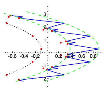
Since δ∞D​P​(t)∈[12,1]\delta_{\infty}^{DP}(t)\in[\frac{1}{2},1], the path γa,b\gamma_{a,b} is contained between the graphs of two parabolas with horizontal distance 12\frac{1}{2}, see Figure 2.

Refer to caption
Figure 2. The path γa,b​(t)\gamma_{a,b}(t) (blue) and the central charges Z⁡(E)r⁡(E)\frac{Z(E)}{r(E)} of exceptional vector bundles EE (red)
Lemma 4.1.

Let ℱ∈Cohℙ2\mathcal{F}\in\mathop{\mathrm{Coh}}\nolimits\mathbb{P}^{2} be a torsion-free slope-stable sheaf on ℙ2\mathbb{P}^{2} of rank rr that is not an exceptional vector bundle. Then Za,b​(i∗​ℱ)r∈Sa,b\frac{Z_{a,b}(i_{*}\mathcal{F})}{r}\in S_{a,b}.

Proof. We write ch(ℱ)r=[ℙ2]+μ⁡[l]+cr​[pt]\frac{\mathop{\mathrm{ch}}\nolimits(\mathcal{F})}{r}=[\mathbb{P}^{2}]+\mu[l]+\frac{c}{r}[\mathrm{pt}] and Za,b​(i∗​ℱ)r=x+i​y\frac{Z_{a,b}(i_{*}\mathcal{F})}{r}=x+iy. Using Theorem 2.3, we obtain:

y\displaystyle y =ℑ⁡a​μ+ℑ⁡b\displaystyle=\Im a\mu+\Im b
x\displaystyle x =−cr+ℜ⁡a​μ+ℜ⁡b=Δ⁡(ℱ)−12​μ2+ℜ⁡a​μ+ℜ⁡b\displaystyle=-\frac{c}{r}+\Re a\mu+\Re b=\Delta(\mathcal{F})-\frac{1}{2}\mu^{2}+\Re a\mu+\Re b
≥δ∞D​P​(μ)−12​μ2+ℜ⁡a​μ+ℜ⁡b\displaystyle\geq\delta_{\infty}^{DP}(\mu)-\frac{1}{2}\mu^{2}+\Re a\mu+\Re b

Setting t=μt=\mu yields the claim. □\Box

Lemma 4.2.

For any (a,b)∈G(a,b)\in G, the central charge Za,bZ_{a,b} is a stability function for Coh0♯⁡(B)\mathop{\mathrm{Coh}}\nolimits_{0}^{\sharp(B)}: if 0≠E∈Coh0♯⁡(B)0\neq E\in\mathop{\mathrm{Coh}}\nolimits_{0}^{\sharp(B)}, then Za,b​(E)∈ℍZ_{a,b}(E)\in\mathbb{H}.

Proof. It is sufficient to prove the claim for torsion sheaves of dimension ≤1\leq 1, and for (shifts of) slope-stable sheaves. The claim is only non-trivial for objects ℱ⁡[1]\mathcal{F}[1], where ℱ\mathcal{F} is a purely 22-dimensional slope-stable of slope μ⁡(ℱ)=B\mu(\mathcal{F})=B. In such a case, Za,b​(ℱ)Z_{a,b}(\mathcal{F}) is lying on the real line. By Lemma 3.1, ℱ\mathcal{F} is the push-forward of a slope-stable sheaf on ℙ2\mathbb{P}^{2}. If ℱ\mathcal{F} is not an exceptional vector bundle, the previous lemma shows Za,b​(i∗​ℱ)∈ℝ>0Z_{a,b}(i_{*}\mathcal{F})\in\mathbb{R}_{>0}. If it is exceptional, the same computation yields this statement from inequality (3). □\Box

In other words, inequality (2) is equivalent to 0∉Sa,b0\notin S_{a,b}, i.e., the path is passing through the real line with positive real part; and inequality (3) is equivalent to Z⁡(ℰ)∉ℝ≤0Z(\mathcal{E})\not\in\mathbb{R}_{\leq 0} for any exceptional vector bundle ℰ\mathcal{E} on ℙ2\mathbb{P}^{2}. Together, they guarantee that the central charge of a slope-stable sheaf never lies on the negative real line.

Due to the above Lemma, as in Remark B.1 we can define a phase function ϕ⁡(E):=(1/π)​arg⁡(Z⁡(E))∈(0,1]\phi(E):=(1/\pi)\arg(Z(E))\in(0,1], for all 0≠E∈Coh0♯⁡(B)0\neq E\in\mathop{\mathrm{Coh}}\nolimits_{0}^{\sharp(B)}.

Lemma 4.3 ([Bri08, Proposition 7.1]).

Let a,b∈ℂa,b\in\mathbb{C} be such that B∈ℚB\in\mathbb{Q} and Za,b(Coh0♯⁡(B)∖{0})⊂ℍZ_{a,b}(\mathop{\mathrm{Coh}}\nolimits_{0}^{\sharp(B)}\setminus\{0\})\subset\mathbb{H}. Then Harder-Narasimhan filtrations exist for (Za,b,Coh0♯⁡(B))(Z_{a,b},\mathop{\mathrm{Coh}}\nolimits_{0}^{\sharp(B)}).

Proof. We use Proposition B.2. Since B∈ℚB\in\mathbb{Q}, the image of ℑ⁡(Za,b)\Im(Z_{a,b}) is discrete in ℝ\mathbb{R}.

Let F∈Coh0♯⁡(B)F\in\mathop{\mathrm{Coh}}\nolimits_{0}^{\sharp(B)} and let

(6) 0=A0⊂A1⊂…⊂Aj⊂Aj+1⊂…⊂F,0=A_{0}\subset A_{1}\subset\ldots\subset A_{j}\subset A_{j+1}\subset\ldots\subset F,

be a sequence of subobjects, with Aj∈𝒫a,b′​(1)A_{j}\in\mathcal{P}^{\prime}_{a,b}(1). As in Proposition B.2, 𝒫a,b′​(1)\mathcal{P}^{\prime}_{a,b}(1) is the full subcategory of Coh0♯⁡(B)\mathop{\mathrm{Coh}}\nolimits_{0}^{\sharp(B)} whose objects have phase 11 with respect to Za,bZ_{a,b}. We need to show that (6) stabilizes.

To this end, we first observe that (6) induces a sequence of inclusions

(7) 0=ℋ−1​(A0)↪…​ℋ−1​(Aj)↪…↪ℋ−1​(F).0=\mathcal{H}^{-1}(A_{0})\hookrightarrow\ldots\mathcal{H}^{-1}(A_{j})\hookrightarrow\ldots\hookrightarrow\mathcal{H}^{-1}(F).

Since Coh0\mathop{\mathrm{Coh}}\nolimits_{0} is Noetherian, (7) must terminate. We can therefore assume that ℋ−1​(Aj)≅ℱ−1\mathcal{H}^{-1}(A_{j})\cong\mathcal{F}_{-1} for all jj and some ℱ−1∈Coh0≤B\mathcal{F}_{-1}\in\mathop{\mathrm{Coh}}\nolimits_{0}^{\leq B}. Let ℱ0\mathcal{F}_{0} denote the cokernel of the inclusion ℱ−1↪ℋ−1​(F)\mathcal{F}_{-1}\hookrightarrow\mathcal{H}^{-1}(F); then, by the long exact cohomology sequence, we have ℱ0∈Coh0≤B\mathcal{F}_{0}\in\mathop{\mathrm{Coh}}\nolimits_{0}^{\leq B} as well.

Now, observe that the simple objects of 𝒫a,b′​(1)\mathcal{P}^{\prime}_{a,b}(1) are skyscraper sheaves k⁡(x)k(x) (x∈ℙ2x\in\mathbb{P}^{2}) and objects of the form i∗​𝒢​[1]i_{*}\mathcal{G}[1], for 𝒢∈Cohℙ2\mathcal{G}\in\mathop{\mathrm{Coh}}\nolimits\mathbb{P}^{2} a locally-free slope-stable sheaf on ℙ2\mathbb{P}^{2} with μ⁡(𝒢)=B\mu(\mathcal{G})=B. Indeed, this can be proved in precisely the same way as Lemma 3.2, (c). In particular, ℋ0​(Aj)\mathcal{H}^{0}(A_{j}) is a torsion sheaf of dimension zero.

Let BjB_{j} be the cokernel in Coh0♯⁡(B)\mathop{\mathrm{Coh}}\nolimits_{0}^{\sharp(B)} of Aj↪FA_{j}\hookrightarrow F; then we have an exact sequence

0→ℱ0→fjℋ−1​(Bj)→ℋ0​(Aj)→gjℋ0​(F).0\to\mathcal{F}_{0}\stackrel{{\scriptstyle f_{j}}}{{\to}}\mathcal{H}^{-1}(B_{j})\to\mathcal{H}^{0}(A_{j})\stackrel{{\scriptstyle g_{j}}}{{\to}}\mathcal{H}^{0}(F).

The cokernel cokerfj\mathop{\mathrm{coker}}f_{j} is zero-dimensional; since ℱ0\mathcal{F}_{0} is fixed ℋ−1​(Bj)\mathcal{H}^{-1}(B_{j}) is pure of dimension 22, the length of cokerfj\mathop{\mathrm{coker}}f_{j} is bounded. As the length of the image imgj\mathop{\mathrm{im}}\nolimits g_{j} is also bounded, we get a bound on the length of ℋ0​(Aj)\mathcal{H}^{0}(A_{j}). At the same time, if DjD_{j} denotes the cokernel in Coh0♯⁡(B)\mathop{\mathrm{Coh}}\nolimits_{0}^{\sharp(B)} of Aj↪Aj+1A_{j}\hookrightarrow A_{j+1}, we must have ℋ−1​(Dj)=0\mathcal{H}^{-1}(D_{j})=0, and thus an inclusion ℋ0​(Aj)↪ℋ0​(Aj+1)\mathcal{H}^{0}(A_{j})\hookrightarrow\mathcal{H}^{0}(A_{j+1}). Hence, for j≫0j\gg 0, ℋ0​(Aj)≅ℋ0​(Aj+1)\mathcal{H}^{0}(A_{j})\cong\mathcal{H}^{0}(A_{j+1}) and so (6) stabilizes. □\Box

Notice that, in the assumptions of Lemma 4.3, the pair (Za,b,Coh0♯⁡(B))(Z_{a,b},\mathop{\mathrm{Coh}}\nolimits_{0}^{\sharp(B)}) defines a locally-finite stability condition on 𝒟0\mathcal{D}_{0}. Indeed this follows immediately from [Bri08, Lemma 4.4].

In the rest of this section, we will use Bridgeland’s deformation result to extend the existence of Harder-Narasimhan filtrations to the case where a,ba,b are not rational. In order to make the deformation effective, we need to bound the metric ∥⋅∥σa,b\|\cdot\|_{\sigma_{a,b}} on Hom(K⁡(𝒟0),ℂ)≅ℂ3\mathop{\mathrm{Hom}}\nolimits(K(\mathcal{D}_{0}),\mathbb{C})\cong\mathbb{C}^{3} defined in equation (5) relative to an arbitrarily chosen metric, with the bound depending continuously on a,b∈Ga,b\in G.

We define the following functions G→ℝ≥0G\to\mathbb{R}_{\geq 0}:

γmin​(a,b)\displaystyle\gamma_{\mathop{\mathrm{min}}\nolimits}(a,b) :=inf{|γa,b​(t)|:t∈ℝ}\displaystyle:=\mathop{\mathrm{inf}}\nolimits\left\{\left\lvert\gamma_{a,b}(t)\right\rvert\,\colon\,t\in\mathbb{R}\right\}
Emin​(a,b)\displaystyle E_{\mathop{\mathrm{min}}\nolimits}(a,b) :=inf{|Za,b​(ℰ)r⁡(ℰ)+t|:t∈ℝ≥0, ℰ exceptional v. bundle}\displaystyle:=\mathop{\mathrm{inf}}\nolimits\left\{\left\lvert\frac{Z_{a,b}(\mathcal{E})}{r(\mathcal{E})}+t\right\rvert\,\colon\,\text{$t\in\mathbb{R}_{\geq 0}$, $\mathcal{E}$ exceptional v. bundle}\right\}
Smin​(a,b)\displaystyle S_{\mathop{\mathrm{min}}\nolimits}(a,b) :=min(γmin​(a,b),Emin​(a,b)).\displaystyle:=\mathop{\mathrm{min}}\nolimits(\gamma_{\mathop{\mathrm{min}}\nolimits}(a,b),E_{\mathop{\mathrm{min}}\nolimits}(a,b)).
Lemma 4.4.

The function SminS_{\mathop{\mathrm{min}}\nolimits} is continuous and satisfies

0<Smin(a,b)≤inf{|Za,b​(ℱ)r⁡(ℱ)+t|:t∈ℝ≥0,ℱ∈Coh0slope-stable}0<S_{\mathop{\mathrm{min}}\nolimits}(a,b)\leq\mathop{\mathrm{inf}}\nolimits\left\{\left\lvert\frac{Z_{a,b}(\mathcal{F})}{r(\mathcal{F})}+t\right\rvert\,\colon\,t\in\mathbb{R}_{\geq 0},\,\mathcal{F}\in\mathop{\mathrm{Coh}}\nolimits_{0}\,\mathrm{slope}\text{-}\mathrm{stable}\right\}

for all (a,b)∈G(a,b)\in G.

Proof. The path γa,b​(t)\gamma_{a,b}(t) depends continuously on a,b,ta,b,t and has the properties γa,b​(t)≠0\gamma_{a,b}(t)\neq 0 for all a,b,ta,b,t, and limt→±∞|γa,b​(t)|=+∞\lim_{t\to\pm\infty}\left\lvert\gamma_{a,b}(t)\right\rvert=+\infty. It follows that γmin\gamma_{\mathop{\mathrm{min}}\nolimits} is a positive continuous function.

Since Za,b​(ℰ)∉ℝ≤0Z_{a,b}(\mathcal{E})\not\in\mathbb{R}_{\leq 0}, the term inf{|Za,b​(ℰ)r⁡(ℰ)+t|:t∈ℝ≥0}\mathop{\mathrm{inf}}\nolimits\left\{\left\lvert\frac{Z_{a,b}(\mathcal{E})}{r(\mathcal{E})}+t\right\rvert\,\colon\,t\in\mathbb{R}_{\geq 0}\right\} is positive for every exceptional vector bundle ℰ\mathcal{E} on ℙ2\mathbb{P}^{2}. Further, Theorem 2.3 together with the computation of Lemma 4.1 shows that every accumulation point of the set

{Za,b​(ℰ)r⁡(ℰ):ℰ exceptional v. bdle}\left\{\frac{Z_{a,b}(\mathcal{E})}{r(\mathcal{E})}\,\colon\,\text{$\mathcal{E}$ exceptional v. bdle}\right\}

is contained in Sa,bS_{a,b}. Hence EminE_{\mathop{\mathrm{min}}\nolimits} is also a positive continuous function.

It remains to prove Smin​(a,b)≤|Za,b​(ℱ)r⁡(ℱ)+t|S_{\mathop{\mathrm{min}}\nolimits}(a,b)\leq\left\lvert\frac{Z_{a,b}(\mathcal{F})}{r(\mathcal{F})}+t\right\rvert for all ℱ,t\mathcal{F},t. It holds by definition when ℱ\mathcal{F} is an exceptional vector bundle. Otherwise, the claim follows as Za,b​(ℱ)r⁡(ℱ)+t\frac{Z_{a,b}(\mathcal{F})}{r(\mathcal{F})}+t is contained in Sa,bS_{a,b}. □\Box

Let |⋅|∞\left\lvert\cdot\right\rvert_{\infty} be the supremums-norm on K⁡(𝒟0)⊗ℝ≅ℝ3K(\mathcal{D}_{0})\otimes\mathbb{R}\cong\mathbb{R}^{3} in the coordinates (r,d,c)(r,d,c), i.e., |(r,d,c)|∞=max⁡{|r|,|d|,|c|}\left\lvert(r,d,c)\right\rvert_{\infty}=\max\{\left\lvert r\right\rvert,\left\lvert d\right\rvert,\left\lvert c\right\rvert\}. Let M⁡(a,b)M(a,b) be the matrix

M⁡(a,b):=(100ℑ⁡bℑ⁡a0ℜ⁡bℜ⁡a−1),M(a,b):=\begin{pmatrix}1&0&0\\ \Im b&\Im a&0\\ \Re b&\Re a&-1\end{pmatrix},

and let N⁡(a,b):=‖M​(a,b)−1‖∞N(a,b):=\left\|M(a,b)^{-1}\right\|_{\infty} be the norm of its inverse, where ‖⋅‖∞\left\|\cdot\right\|_{\infty} is the operator norm with respect to the supremums-norm on ℝ3\mathbb{R}^{3}. We claim the following estimate, which is the “support property” discussed in Proposition B.4 with an explicit constant:

Lemma 4.5.

If E∈Coh0♯⁡(B)E\in\mathop{\mathrm{Coh}}\nolimits_{0}^{\sharp(B)} is Za,bZ_{a,b}-stable, then

|Za,b​(E)||E|∞≥min(Smin​(a,b),1)N⁡(a,b).\frac{\left\lvert Z_{a,b}(E)\right\rvert}{\left\lvert E\right\rvert_{\infty}}\geq\frac{\mathop{\mathrm{min}}\nolimits\left(S_{\mathop{\mathrm{min}}\nolimits}(a,b),1\right)}{N(a,b)}.

We first show how to conclude the proof of Theorem 2.5 from the lemma:

Corollary 4.6.

There exists a geometric stability condition σa,b\sigma_{a,b} for arbitrary pairs (a,b)∈G⊂ℂ2(a,b)\in G\subset\mathbb{C}^{2}.

Proof. Let V⊂UV\subset U be the subset of geometric stability conditions σ=(Z,𝒫)\sigma=(Z,\mathcal{P}) such that all skyscraper sheaves k⁡(x)k(x) are stable of phase 11 with Z⁡(k⁡(x))=−1Z(k(x))=-1. For any such stability condition, the central charge is of the form Z=Za,bZ=Z_{a,b} of equation (4), and thus 𝒵\mathcal{Z} induces a map 𝒵V:V→ℂ2,σ↦(a,b)\mathcal{Z}_{V}\colon V\to\mathbb{C}^{2},\sigma\mapsto(a,b).

As proved at the end of Section 3, the heart of such a stability condition is uniquely determined; thus 𝒵V\mathcal{Z}_{V} is injective, and so it is a homeomorphism onto its image. Using Corollary 3.4 and the deformation property, we see that the image of 𝒵V\mathcal{Z}_{V} is open in ℂ2\mathbb{C}^{2}. By Lemma 4.3 and Lemma 4.5 (which shows that the stability conditions satisfy condition (b) in Definition 2.1), it contains the dense subset of (a,b)∈G(a,b)\in G such that B=−ℑ⁡bℑ⁡a∈ℚB=-\frac{\Im b}{\Im a}\in\mathbb{Q} is rational. Hence it suffices to prove that the image is closed in GG.

Assume the contrary, and that (a,b)∈G(a,b)\in G are in the boundary of 𝒵V\mathcal{Z}_{V}. By Lemma 4.4 the function SminS_{\mathop{\mathrm{min}}\nolimits} is continuous and positive. It follows that for all (a′,b′)∈G(a^{\prime},b^{\prime})\in G sufficiently close to (a,b)(a,b), we have

‖Za,b−Za′,b′‖∞<sin⁡(π8)​min(Smin​(a′,b′),1)N⁡(a′,b′).\left\|Z_{a,b}-Z_{a^{\prime},b^{\prime}}\right\|_{\infty}<\sin\left(\frac{\pi}{8}\right)\frac{\mathop{\mathrm{min}}\nolimits\left(S_{\mathop{\mathrm{min}}\nolimits}(a^{\prime},b^{\prime}),1\right)}{N(a^{\prime},b^{\prime})}.

By the definition of ∥⋅∥σa′,b′\|\cdot\|_{\sigma_{a^{\prime},b^{\prime}}} (see equation (5)) and Lemma 4.5, this implies

‖Za,b−Za′,b′‖σa′,b′<sin⁡(π8)\left\|Z_{a,b}-Z_{a^{\prime},b^{\prime}}\right\|_{\sigma_{a^{\prime},b^{\prime}}}<\sin\left(\frac{\pi}{8}\right)

for all such (a′,b′)(a^{\prime},b^{\prime}) for which a geometric stability condition σa′,b′\sigma_{a^{\prime},b^{\prime}} exists.

By Bridgeland’s effective deformation result (see Theorem B.3) there exists a stability condition σa,b=(Za,b,𝒫a,b)\sigma_{a,b}=(Z_{a,b},\mathcal{P}_{a,b}) in the neighborhood of σa′,b′\sigma_{a^{\prime},b^{\prime}}. By choosing (a′,b′)(a^{\prime},b^{\prime}) appropriately, we may assume that σa,b\sigma_{a,b} is on one of the walls in the sense of Corollary 3.4; in particular, k⁡(x)k(x) is semistable, and there is an inclusion E↪k⁡(x)E\hookrightarrow k(x) in 𝒫a,b​(1)\mathcal{P}_{a,b}(1) with EE being stable. In particular, 0=ℑ⁡Za,b​(E)=ℑ⁡a⋅d⁡(E)+ℑ⁡b⋅r⁡(E)0=\Im Z_{a,b}(E)=\Im a\cdot d(E)+\Im b\cdot r(E). Since k⁡(x)k(x) is stable with respect to σa′,b′\sigma_{a^{\prime},b^{\prime}}, we have ℑ⁡Za′,b′​(E)≠0\Im Z_{a^{\prime},b^{\prime}}(E)\neq 0, and thus we have r⁡(E)≠0r(E)\neq 0 or d⁡(E)≠0d(E)\neq 0. Since ℑ⁡a>0\Im a>0, it follows that r⁡(E)≠0r(E)\neq 0; but then B=−ℑ⁡bℑ⁡a=d⁡(E)r⁡(E)∈ℚB=-\frac{\Im b}{\Im a}=\frac{d(E)}{r(E)}\in\mathbb{Q}, and so we already know that there exists a geometric stability condition σ∈V\sigma\in V with 𝒵V​(σ)=(a,b)\mathcal{Z}_{V}(\sigma)=(a,b). □\Box

Proof. (Lemma 4.5) Writing r=r⁡(E)r=r(E) etc., we have

|E|∞\displaystyle\left\lvert E\right\rvert_{\infty} =max⁡(r,d,c)\displaystyle=\max(r,d,c)
=|M​(a,b)−1⋅(r,ℑ⁡a⋅d+ℑ⁡b⋅r,−c+ℜ⁡a⋅d+ℜ⁡b⋅r)|∞\displaystyle=\left\lvert M(a,b)^{-1}\cdot\bigl(r,\Im a\cdot d+\Im b\cdot r,-c+\Re a\cdot d+\Re b\cdot r\bigr)\right\rvert_{\infty}
≤N⁡(a,b)⋅|(r,ℑ⁡Za,b​(E),ℜ⁡Za,b​(E))|∞\displaystyle\leq N(a,b)\cdot\left\lvert\left(r,\Im Z_{a,b}(E),\Re Z_{a,b}(E)\right)\right\rvert_{\infty}
≤N⁡(a,b)⋅max⁡(|r|,|Za,b​(E)|)\displaystyle\leq N(a,b)\cdot\max(\left\lvert r\right\rvert,\left\lvert Z_{a,b}(E)\right\rvert)

Thus the claim follows if we can show

|Z¯​(E)|>Smin(a,b)\left\lvert\overline{Z}(E)\right\rvert>S_{\mathop{\mathrm{min}}\nolimits(a,b)}

where E∈Coh0♯⁡(B)E\in\mathop{\mathrm{Coh}}\nolimits_{0}^{\sharp(B)} is any Za,bZ_{a,b}-stable objects with non-zero rank, and where we wrote Z¯​(E)=Za,b​(E)|r⁡(E)|\overline{Z}(E)=\frac{Z_{a,b}(E)}{\left\lvert r(E)\right\rvert}.

Assume first that r⁡(H0​(E))≥r⁡(H−1​(E))r(H^{0}(E))\geq r(H^{-1}(E)), with r​(H0​(E))>0r(H^{0}(E))>0. We have

ℑ⁡Za,b​(E)≥ℑ⁡Za,b​(H0​(E)),\Im Z_{a,b}(E)\geq\Im Z_{a,b}(H^{0}(E)),

as E↠H0​(E)E\twoheadrightarrow H^{0}(E) is a quotient in Coh0♯⁡(B)\mathop{\mathrm{Coh}}\nolimits_{0}^{\sharp(B)} and Za,bZ_{a,b} is a stability function, and we have |r⁡(E)|≤r⁡(H0​(E))\left\lvert r(E)\right\rvert\leq r(H^{0}(E)); together, they show

ℑ⁡Z¯​(E)≥ℑ⁡Z¯​(H0​(E)).\Im\overline{Z}(E)\geq\Im\overline{Z}(H^{0}(E)).

Let H0​(E)↠ℱH^{0}(E)\twoheadrightarrow\mathcal{F} be a semistable quotient with μ⁡(H0​(E))≥μ⁡(ℱ)>B\mu(H^{0}(E))\geq\mu(\mathcal{F})>B (such a quotient always exists due to the existence of HN-filtrations for slope stability). Then

ℑ⁡Z¯​(H0​(E))\displaystyle\Im\overline{Z}(H^{0}(E)) =ℑ⁡a⋅d⁡(H0​(E))+ℑ⁡b⋅r⁡(H0​(E))r​(H0​(E))=ℑ⁡a⁡(μ⁡(H0​(E))−B)\displaystyle=\frac{\Im a\cdot d(H^{0}(E))+\Im b\cdot r(H^{0}(E))}{r(H^{0}(E))}=\Im a\left(\mu(H^{0}(E))-B\right)
≥ℑ⁡a⁡(μ⁡(ℱ)−B)=ℑ⁡Z¯​(ℱ)\displaystyle\geq\Im a\left(\mu(\mathcal{F})-B\right)=\Im\overline{Z}(\mathcal{F})

(where we used the assumption ℑ⁡a>0\Im a>0 in the inequality).

On the other hand, as EE is Za,bZ_{a,b}-semistable and ℱ∈Coh0♯⁡(B)\mathcal{F}\in\mathop{\mathrm{Coh}}\nolimits_{0}^{\sharp(B)}, and so the phase of Za,b​(ℱ)Z_{a,b}(\mathcal{F}) is at least as big as the phase of Za,b​(E)Z_{a,b}(E). Hence the line segment connecting 0 and Z¯​(E)\overline{Z}(E) intersects the ray Z¯​(ℱ)+t,t≥0\overline{Z}(\mathcal{F})+t,t\geq 0 (see Figure 3). By Lemma 4.4, this implies the claim.

Refer to caption
Figure 3. Location of Z¯​(ℱ)\overline{Z}(\mathcal{F}) relative to Z¯​(E)\overline{Z}(E)

A dual argument holds in case r⁡(H−1​(E))>r⁡(H0​(E))r(H^{-1}(E))>r(H^{0}(E)), by considering a slope-stable sheaf ℱ↪H−1​(E)\mathcal{F}\hookrightarrow H^{-1}(E) with B≥μ⁡(ℱ)≥μ⁡(H−1​(E))B\geq\mu(\mathcal{F})\geq\mu(H^{-1}(E)). Finally, when H−1​(E)H^{-1}(E) is zero and H0​(E)H^{0}(E) has rank zero, there is nothing to prove. □\Box

Remark 4.7.

The methods used in the last part of this section also apply in the situation [ABL07, Section 2]: the stability conditions constructed there for rational divisors D,FD,F deform to produce stability condition for arbitrary ℝ\mathbb{R}-divisors D,FD,F with FF ample.

5. Boundary of the geometric chamber

In this section we will show that the set of boundary walls of the geometric chamber UU can be described explicitly using exceptional vector bundles ℰ\mathcal{E} on ℙ2\mathbb{P}^{2}. For any such ℰ\mathcal{E}, the push-forward i∗​ℰi_{*}\mathcal{E} is a spherical object in 𝒟0\mathcal{D}_{0}. We denote by STℰ:𝒟0→𝒟0{\mathop{\mathrm{ST}}\nolimits}_{\mathcal{E}}\colon\mathcal{D}_{0}\to\mathcal{D}_{0} the spherical twist at i∗​ℰi_{*}\mathcal{E}. If rr is the rank of ℰ\mathcal{E} and x∈ℙ2x\in\mathbb{P}^{2}, we also write ℰx\mathcal{E}^{x} for the kernel of the natural map i∗​ℰ⊕r↠k⁡(x)i_{*}\mathcal{E}^{\oplus r}\twoheadrightarrow k(x).

The goal of this section is to prove the following theorem:

Theorem 5.1.

For every exceptional vector bundle ℰ\mathcal{E} there exist two codimension one walls Wℰ+,Wℰ−⊂∂UW_{\mathcal{E}}^{+},W_{\mathcal{E}}^{-}\subset\partial U with the following properties:

  1. (a)

    Stability conditions in Wℰ+W_{\mathcal{E}}^{+} are characterized by the property that i∗​ℰi_{*}\mathcal{E} and all skyscraper sheaves k⁡(x)k(x) are semistable of the same phase ϕ\phi, with i∗​ℰi_{*}\mathcal{E} being a subobject of k⁡(x)k(x) in 𝒫⁡(ϕ)\mathcal{P}(\phi); at a general point of Wℰ+W_{\mathcal{E}}^{+}, the Jordan-Hölder filtration of any skyscraper sheaf k⁡(x)k(x) is given by

    (8) i∗​ℰ⊕r→k⁡(x)→ℰx​[1].i_{*}\mathcal{E}^{\oplus r}\to k(x)\to\mathcal{E}^{x}[1].

    Similarly, we have σ∈Wℰ−\sigma\in W_{\mathcal{E}}^{-} if i∗​ℰ​[2]i_{*}\mathcal{E}[2] is semistable of the same phase ϕ\phi as k⁡(x)k(x), and i∗​ℰ​[2]i_{*}\mathcal{E}[2] is a quotient of k⁡(x)k(x) in 𝒫⁡(ϕ)\mathcal{P}(\phi). At a general point in Wℰ−W_{\mathcal{E}}^{-}, the Jordan-Hölder filtration of k⁡(x)k(x) is given by

    (9) STℰ−1(ℰx​[1])→k⁡(x)→i∗​ℰ⊕r​[2].{\mathop{\mathrm{ST}}\nolimits}_{\mathcal{E}}^{-1}(\mathcal{E}^{x}[1])\to k(x)\to i_{*}\mathcal{E}^{\oplus r}[2].
  2. (b)

    We have Wℰ+=U¯∩STℰ(U¯)W_{\mathcal{E}}^{+}=\overline{U}\cap{\mathop{\mathrm{ST}}\nolimits}_{\mathcal{E}}\left(\overline{U}\right), i.e., Wℰ+W_{\mathcal{E}}^{+} is the wall between UU and STℰ(U){\mathop{\mathrm{ST}}\nolimits}_{\mathcal{E}}(U); similarly, Wℰ−=U¯∩STℰ−1(U¯)W_{\mathcal{E}}^{-}=\overline{U}\cap{\mathop{\mathrm{ST}}\nolimits}_{\mathcal{E}}^{-1}\left(\overline{U}\right).

There are no other walls in ∂U\partial U.

Corollary 5.2.

The translates of U¯\overline{U} under the group of autoequivalences generated by STℰ{\mathop{\mathrm{ST}}\nolimits}_{\mathcal{E}} cover the whole connected component Stab†(𝒟0)\mathop{\mathrm{Stab}}^{{\dagger}}(\mathcal{D}_{0}) of UU in the space of stability conditions.

Proof. Let α:[0,1]→Stab(𝒟0)\alpha\colon[0,1]\to\mathop{\mathrm{Stab}}(\mathcal{D}_{0}) be a path of stability conditions with α⁡(0)∈U\alpha(0)\in U. By Proposition 3.3, there exists a finite set of walls Wi[k⁡(x)]W^{[k(x)]}_{i} intersecting α\alpha, such that the set of stable objects of class [k⁡(x)][k(x)] is constant in the complement of the intersection points. We may also assume that α\alpha intersects each wall transversely and in a generic point of the wall. Using the above theorem, it follows by induction that every open interval in the complement is contained in the translate of UU under a sequence of spherical twists. □\Box

Most of the existing proofs of statements similar to the above claims are in the situation of a Calabi-Yau 2-category. In that situation, Lemma 5.2 of [Bri08] applies, which guarantees, via an Euler characteristic computation, that every non-trivial Harder-Narasimhan filtration of a skyscraper sheaf k⁡(x)k(x) contains a spherical object. In a Calabi-Yau 3-category, spherical objects cannot be characterized via their Euler characteristic among stable objects. Instead, our proof is obtained by a direct geometric analysis of the boundary of UU.

Consider a stability condition (Z,𝒫)(Z,\mathcal{P}) in the boundary ∂U\partial U of UU. Since the skyscraper sheaves k⁡(x)k(x) are semistable, ZZ satisfies Z⁡(k⁡(x))≠0Z(k(x))\neq 0 and, up to the action of ℂ\mathbb{C}, we can still assume k⁡(x)∈𝒫⁡(1)k(x)\in\mathcal{P}(1) and Z=Za,bZ=Z_{a,b} for a,b∈ℂa,b\in\mathbb{C} as in equation (4). By Bridgeland’s deformation result and Theorem 2.5, a,b∈ℂa,b\in\mathbb{C} must satisfy one of the following conditions:

Case aa:

ℑ⁡a=0\Im a=0

Case EE:

ℑ⁡a>0\Im a>0, there exists an exceptional vector bundle of slope B=−ℑ⁡bℑ⁡aB=-\frac{\Im b}{\Im a}, and we have δ∞D​P​(B)>−ℜ⁡b−B⋅ℜ⁡a+12​B2>ΔB\delta_{\infty}^{DP}(B)>-\Re b-B\cdot\Re a+\frac{1}{2}B^{2}>\Delta_{B}.

Case δ∞D​P\delta_{\infty}^{DP}:

ℑ⁡a>0\Im a>0 and −ℜ⁡b−B⋅ℜ⁡a+12​B2=δ∞D​P​(B)-\Re b-B\cdot\Re a+\frac{1}{2}B^{2}=\delta_{\infty}^{DP}(B).

We begin by showing that “Case δ∞D​P\delta_{\infty}^{DP}” cannot exist.

Lemma 5.3.

Let σt=(Zt,𝒫t)\sigma_{t}=(Z_{t},\mathcal{P}_{t}) for t∈I⊂ℝt\in I\subset\mathbb{R} be a path in the space of stability conditions such that ℑ⁡Zt\Im Z_{t} is constant. Then 𝒫t​((0,1])\mathcal{P}_{t}((0,1]) and 𝒫t​(1)\mathcal{P}_{t}(1) are constant, too.

Proof. Let t1,t2∈It_{1},t_{2}\in I be such that σt1\sigma_{t_{1}} and σt2\sigma_{t_{2}} are close with respect to the metric on Stab(𝒟0)\mathop{\mathrm{Stab}}(\mathcal{D}_{0}); to be specific, we assume d⁡(σt1,σt2)<18d(\sigma_{t_{1}},\sigma_{t_{2}})<\frac{1}{8}. Given ϕ∈(0,1]\phi\in(0,1], the objects E∈𝒫t2​(ϕ)E\in\mathcal{P}_{t_{2}}(\phi) can be characterized as the Zt2Z_{t_{2}}-stable objects in the quasi-abelian category 𝒫t1​((,,,))\mathcal{P}_{t_{1}}((\phi-\frac{1}{8},\phi+\frac{1}{8})) (see [Bri07, Section 7]). We want to show E∈𝒫t1​((0,1])E\in\mathcal{P}_{t_{1}}((0,1]).

In case 18≤ϕ≤78\frac{1}{8}\leq\phi\leq\frac{7}{8} we are done. If ϕ∈(78,1]\phi\in(\frac{7}{8},1], then for any A∈𝒫t1​((,,,))A\in\mathcal{P}_{t_{1}}((1,\phi+\frac{1}{8})) we have ℑ⁡Zt2​(A)=ℑ⁡Zt1​(A)<0\Im Z_{t_{2}}(A)=\Im Z_{t_{1}}(A)<0, and thus the phase of AA with respect to Zt2Z_{t_{2}} is bigger than one. Hence AA cannot be a subobject of EE. By considering the Harder-Narasimhan filtration of EE with respect to 𝒫t1\mathcal{P}_{t_{1}}, this implies that E∈𝒫t1((ϕ−18,1])E\in\mathcal{P}_{t_{1}}((\phi-\frac{1}{8},1]). A similar argument applies for 0<ϕ<180<\phi<\frac{1}{8}.

It follows that 𝒫t2​((0,1])⊂𝒫t1​((0,1])\mathcal{P}_{t_{2}}((0,1])\subset\mathcal{P}_{t_{1}}((0,1]), and thus they must be equal. The claim about 𝒫t​(1)\mathcal{P}_{t}(1) follows easily. □\Box

Lemma 5.4.

There are no stability conditions σ=(Za,b,𝒫)\sigma=(Z_{a,b},\mathcal{P}) in ∂U\partial U such that ℑ⁡a>0\Im a>0 and −ℜ⁡b−B⋅ℜ⁡a+12​B2=δ∞D​P​(B)-\Re b-B\cdot\Re a+\frac{1}{2}B^{2}=\delta_{\infty}^{DP}(B).

Proof. Due to Corollary 3.4, we may assume that BB is irrational.

Consider the path σt=(Za⁡(t),b⁡(t),𝒫t),t∈[0,1]\sigma_{t}=(Z_{a(t),b(t)},\mathcal{P}_{t}),t\in[0,1] in Stab(𝒟0)\mathop{\mathrm{Stab}}(\mathcal{D}_{0}) starting at σ\sigma induced by deforming ZZ as Za⁡(t),b⁡(t)Z_{a(t),b(t)}, with a⁡(t)=aa(t)=a constant, and b⁡(t)=b+ϵ​tb(t)=b+\epsilon t. Due to the form of the inequalities in Theorem 2.5, the stability conditions σt\sigma_{t} for t>0t>0 are geometric.

By the previous lemma, it follows that 𝒫0((0,1])=𝒫1((0,1])=Coh0♯⁡(B)\mathcal{P}_{0}((0,1])=\mathcal{P}_{1}((0,1])=\mathop{\mathrm{Coh}}\nolimits_{0}^{\sharp(B)} and, since BB is irrational, that 𝒫0​(1)\mathcal{P}_{0}(1) is generated by the skyscraper sheaves k⁡(x)k(x). The sheaves k⁡(x)k(x) have no subobjects in this category, thus they are stable. By Corollary 3.4, this contradicts the assumption that σ\sigma is in the boundary of UU. □\Box

The following lemma deals with “Case aa”:

Lemma 5.5.

Let (Za,b,𝒫)∈∂U(Z_{a,b},\mathcal{P})\in\partial U be a stability condition with ℑ⁡a=0\Im a=0. Then ℑ⁡b=0\Im b=0, i.e., the image of ZZ is contained in the real line.

Proof. Writing inequality (2) without denominators we get

(ℑ⁡a)2​ℜ⁡b>ℑ⁡a⋅ℑ⁡b⋅ℜ⁡a−(ℑ⁡a)2​δ∞D​P​(B)+12​(ℑ⁡b)2(\Im a)^{2}\Re b>\Im a\cdot\Im b\cdot\Re a-(\Im a)^{2}\delta_{\infty}^{DP}(B)+\frac{1}{2}(\Im b)^{2}

By continuity, this implies (ℑ⁡b)2≤0(\Im b)^{2}\leq 0 on the boundary with ℑ⁡a=0\Im a=0. □\Box

In particular, the part of the boundary with ℑ⁡a=0\Im a=0 is a codimension two subset; by Corollary 3.4, any such point is contained in the closure of the ℑ⁡a>0\Im a>0-part of a wall.

We will now consider boundary stability conditions in “Case EE”. Let a,b,Ba,b,B be as in the assumption, and let ℰ\mathcal{E} be the unique exceptional vector bundle on ℙ2\mathbb{P}^{2} of slope BB (see Theorem A.2); then Za,b​(i∗​ℰ)∈(−1,0)Z_{a,b}(i_{*}\mathcal{E})\in(-1,0) and Za,b​(i∗​𝒢)∈ℝ>0Z_{a,b}(i_{*}\mathcal{G})\in\mathbb{R}_{>0} for any other slope-stable sheaf 𝒢\mathcal{G} on ℙ2\mathbb{P}^{2} of slope BB. This suggests that i∗​ℰi_{*}\mathcal{E} is semistable, of phase ϕ⁡(i∗​ℰ)=±1\phi(i_{*}\mathcal{E})=\pm 1 (depending on whether Z⁡(i∗​ℰ)Z(i_{*}\mathcal{E}) approaches the real line from above or below when we approach Za,bZ_{a,b} by geometric stability conditions); and in the case ϕ⁡(i∗​ℰ)=+1\phi(i_{*}\mathcal{E})=+1, the tt-structure 𝒫⁡((0,1])\mathcal{P}((0,1]) should be given as in the following proposition.

We will prove this by constructing the stability conditions in the boundary directly, and prove that they deform to geometric stability conditions.

Proposition 5.6.

Let BB be the slope of an exceptional vector bundle ℰ\mathcal{E} on ℙ2\mathbb{P}^{2}. Then there is a torsion pair (𝒯ℰ,ℱℰ)(\mathcal{T}^{\mathcal{E}},\mathcal{F}^{\mathcal{E}}) on Coh0\mathop{\mathrm{Coh}}\nolimits_{0} where

  • •

    𝒯ℰ\mathcal{T}^{\mathcal{E}} is the extension-closed subcategory of Coh0\mathop{\mathrm{Coh}}\nolimits_{0} generated by torsion sheaves, by slope-semistable sheaves of slope μ>B\mu>B, and by ℰ\mathcal{E}, and

  • •

    ℱℰ\mathcal{F}^{\mathcal{E}} is generated by slope-semistable sheaves 𝒢\mathcal{G} of slope μ≤B\mu\leq B that also satisfy Hom(i∗​ℰ,𝒢)=0\mathop{\mathrm{Hom}}\nolimits(i_{*}\mathcal{E},\mathcal{G})=0.

Proof. From the construction, it is clear that Hom(𝒯ℰ,ℱℰ)=0\mathop{\mathrm{Hom}}\nolimits(\mathcal{T}^{\mathcal{E}},\mathcal{F}^{\mathcal{E}})=0.

Now given any 𝒢∈Coh0\mathcal{G}\in\mathop{\mathrm{Coh}}\nolimits_{0}, let 𝒢>B↪𝒢↠𝒢≤B\mathcal{G}_{>B}\hookrightarrow\mathcal{G}\twoheadrightarrow\mathcal{G}_{\leq B} the unique short exact sequence with 𝒢>B∈Coh0>B\mathcal{G}_{>B}\in\mathop{\mathrm{Coh}}\nolimits_{0}^{>B} and 𝒢≤B∈Coh0≤B\mathcal{G}_{\leq B}\in\mathop{\mathrm{Coh}}\nolimits_{0}^{\leq B}. Let V=Hom(i∗​ℰ,𝒢≤B)V=\mathop{\mathrm{Hom}}\nolimits(i_{*}\mathcal{E},\mathcal{G}_{\leq B}) and let ℱ\mathcal{F} be the cokernel such that the following sequence is exact on the right:

V⊗i∗​ℰ⟶f𝒢≤B→ℱ→0V\otimes i_{*}\mathcal{E}\stackrel{{\scriptstyle f}}{{\longrightarrow}}\mathcal{G}_{\leq B}\to\mathcal{F}\to 0

We claim that ℱ∈ℱℰ\mathcal{F}\in\mathcal{F}^{\mathcal{E}}, and that the kernel 𝒯\mathcal{T} of the composition 𝒢↠𝒢≤B↠ℱ\mathcal{G}\twoheadrightarrow\mathcal{G}_{\leq B}\twoheadrightarrow\mathcal{F} lies in 𝒯ℰ\mathcal{T}^{\mathcal{E}}.

The image of the evaluation map ff is slope-semistable of slope BB; hence so is the kernel of ff. Since i∗​ℰi_{*}\mathcal{E} is stable, the kernel is of the form i∗​ℰ⊗V′i_{*}\mathcal{E}\otimes V^{\prime} for some V′⊂VV^{\prime}\subset V; by the definition of VV, this forces V′=0V^{\prime}=0, i.e., the above sequence is exact. This shows that 𝒯\mathcal{T} is an extension of 𝒢>B\mathcal{G}_{>B} and i∗​ℰi_{*}\mathcal{E}.

Since Hom(i∗​ℰ,i∗​ℰ)=ℂ\mathop{\mathrm{Hom}}\nolimits(i_{*}\mathcal{E},i_{*}\mathcal{E})=\mathbb{C} and Ext1(i∗​ℰ,i∗​ℰ)=0\mathop{\mathrm{Ext}}\nolimits^{1}(i_{*}\mathcal{E},i_{*}\mathcal{E})=0, the long exact sequence associated to Hom(i∗​ℰ,¯)\mathop{\mathrm{Hom}}\nolimits(i_{*}\mathcal{E},\underline{\hphantom{M}}) shows that Hom(i∗​ℰ,ℱ)=0\mathop{\mathrm{Hom}}\nolimits(i_{*}\mathcal{E},\mathcal{F})=0, and thus ℱ∈ℱℰ\mathcal{F}\in\mathcal{F}^{\mathcal{E}} as desired. □\Box

A similar result as Proposition 5.6 is also in [Yos09, Prop. 2.7].

We continue to assume that a,b∈ℂa,b\in\mathbb{C} satisfy B=−ℑ⁡bℑ⁡aB=-\frac{\Im b}{\Im a} and the inequality of boundary “Case EE”. Let Coh0ℰ=⟨𝒯ℰ,ℱℰ[1]⟩\mathop{\mathrm{Coh}}\nolimits_{0}^{\mathcal{E}}=\langle\mathcal{T}^{\mathcal{E}},\mathcal{F}^{\mathcal{E}}[1]\rangle be the tt-structure given by tilting at the torsion pair of Proposition 5.6. From the previous discussion, it follows that Za,bZ_{a,b} is a stability function for Coh0ℰ\mathop{\mathrm{Coh}}\nolimits_{0}^{\mathcal{E}}.

Proposition 5.7.

Harder-Narasimhan filtrations exist for the stability function Za,bZ_{a,b} on Coh0ℰ\mathop{\mathrm{Coh}}\nolimits_{0}^{\mathcal{E}}.

Proof. The proof is similar to Lemma 4.3. Indeed, since B=−ℑ⁡bℑ⁡aB=-\frac{\Im b}{\Im a} is the slope of ℰ\mathcal{E}, it is rational; hence the imaginary part of Za,bZ_{a,b} is discrete, and we can again apply Proposition B.2.

First note that for any A∈𝒫a,b′​(1)A\in\mathcal{P}^{\prime}_{a,b}(1), the sheaf ℋ0​(A)\mathcal{H}^{0}(A) is in the category extension-generated by k⁡(x),x∈ℙ2k(x),x\in\mathbb{P}^{2}, and by i∗​ℰi_{*}\mathcal{E}: otherwise ℋ0​(A)∈𝒯ℰ\mathcal{H}^{0}(A)\in\mathcal{T}^{\mathcal{E}} would have 0<ℑ⁡Z⁡(ℋ0​(A))≤ℑ⁡Z⁡(A)0<\Im Z(\mathcal{H}^{0}(A))\leq\Im Z(A). To adapt the proof of Lemma 4.3 (where instead we knew that ℋ0​(A)\mathcal{H}^{0}(A) is a zero-dimensional torsion sheaf), we replace all arguments using the length of a maximal zero-dimensional subsheaf by using the function

e:Coh0→ℤ,e(⋅):=dim(Hom(i∗ℰ,⋅)).e\colon\mathop{\mathrm{Coh}}\nolimits_{0}\to\mathbb{Z},\quad e(\cdot):=\mathop{\mathrm{dim}}\nolimits(\mathop{\mathrm{Hom}}\nolimits(i_{*}\mathcal{E},\cdot)).

In many respects, it has the same formal properties needed (e.g. subadditivity on short exact sequences), and the proof goes through:

Assume that F∈Coh0ℰF\in\mathop{\mathrm{Coh}}\nolimits_{0}^{\mathcal{E}} has an infinite sequence

(10) 0=A0⊂A1⊂…⊂Aj⊂Aj+1⊂…⊂F,0=A_{0}\subset A_{1}\subset\ldots\subset A_{j}\subset A_{j+1}\subset\ldots\subset F,

of subobjects with Aj∈𝒫a,b′​(1)A_{j}\in\mathcal{P}^{\prime}_{a,b}(1). Denote by BjB_{j} the cokernel in Coh0ℰ\mathop{\mathrm{Coh}}\nolimits_{0}^{\mathcal{E}} of Aj↪FA_{j}\hookrightarrow F.

By arguing as in Lemma 4.3, we can assume ℋ−1​(Aj)=ℱ−1\mathcal{H}^{-1}(A_{j})=\mathcal{F}_{-1} and ℋ0​(Bj)=𝒢1\mathcal{H}^{0}(B_{j})=\mathcal{G}_{1}, for some ℱ−1,𝒢1∈Coh0\mathcal{F}_{-1},\mathcal{G}_{1}\in\mathop{\mathrm{Coh}}\nolimits_{0} and for all jj. Let ℱ0\mathcal{F}_{0} be the cokernel in Coh0\mathop{\mathrm{Coh}}\nolimits_{0} of ℱ−1↪ℋ−1​(F)\mathcal{F}_{-1}\hookrightarrow\mathcal{H}^{-1}(F) and let 𝒢0\mathcal{G}_{0} be the kernel of ℋ0​(F)↠𝒢1\mathcal{H}^{0}(F)\twoheadrightarrow\mathcal{G}_{1}. Then we have an exact sequence

0→ℱ0→gℋ−1​(Bj)→ℋ0​(Aj)→f𝒢0→0,0\to\mathcal{F}_{0}\stackrel{{\scriptstyle g}}{{\to}}\mathcal{H}^{-1}(B_{j})\to\mathcal{H}^{0}(A_{j})\stackrel{{\scriptstyle f}}{{\to}}\mathcal{G}_{0}\to 0,

and we let 𝒦j=ker⁡f=cokerg\mathcal{K}_{j}=\ker f=\mathop{\mathrm{coker}}g. By the long exact Hom\mathop{\mathrm{Hom}}\nolimits-sequences, we have

e⁡(ℋ0​(Aj))≤e⁡(𝒦j)+e⁡(𝒢0)≤e⁡(ℋ−1​(Bj))+dimExt1(i∗​ℰ,ℱ0)+e⁡(𝒢0).e(\mathcal{H}^{0}(A_{j}))\leq e(\mathcal{K}_{j})+e(\mathcal{G}_{0})\leq e(\mathcal{H}^{-1}(B_{j}))+\mathop{\mathrm{dim}}\nolimits\mathop{\mathrm{Ext}}\nolimits^{1}(i_{*}\mathcal{E},\mathcal{F}_{0})+e(\mathcal{G}_{0}).

By definition of ℱℰ\mathcal{F}^{\mathcal{E}}, we have Hom(i∗​ℰ,ℋ−1​(Bj))=0\mathop{\mathrm{Hom}}\nolimits(i_{*}\mathcal{E},\mathcal{H}^{-1}(B_{j}))=0, and thus e​(ℋ0​(Aj))e(\mathcal{H}^{0}(A_{j})) is bounded.

Now consider a filtration step of (10), and let DjD_{j} be the cokernel in Coh0ℰ\mathop{\mathrm{Coh}}\nolimits_{0}^{\mathcal{E}} of Aj↪Aj+1A_{j}\hookrightarrow A_{j+1}. From the exact sequence

0→ℋ−1​(Dj)→ℋ0​(Aj)→ℋ0​(Aj+1)→ϕℋ0​(Dj)→0,0\to\mathcal{H}^{-1}(D_{j})\to\mathcal{H}^{0}(A_{j})\to\mathcal{H}^{0}(A_{j+1})\stackrel{{\scriptstyle\phi}}{{\to}}\mathcal{H}^{0}(D_{j})\to 0,

we argue similarly as before:

e⁡(ker⁡ϕ)=e⁡(ℋ−1​(Dj))+e⁡(ker⁡ϕ)≥e⁡(ℋ0​(Aj))\displaystyle e(\ker\phi)=e(\mathcal{H}^{-1}(D_{j}))+e(\ker\phi)\geq e(\mathcal{H}^{0}(A_{j}))

On the other hand, as 𝒯ℰ\mathcal{T}^{\mathcal{E}} is closed under quotients, we have ker⁡ϕ∈𝒯ℰ\ker\phi\in\mathcal{T}^{\mathcal{E}}, and thus ker⁡ϕ∈𝒫a,b′​(1)\ker\phi\in\mathcal{P}^{\prime}_{a,b}(1) and Ext1(i∗​ℰ,ker⁡ϕ)=0\mathop{\mathrm{Ext}}\nolimits^{1}(i_{*}\mathcal{E},\ker\phi)=0. Thus we have

e⁡(ℋ0​(Aj+1))=e⁡(ker⁡ϕ)+e⁡(ℋ0​(Dj))≥e⁡(ker⁡ϕ)≥e⁡(ℋ0​(Aj))e(\mathcal{H}^{0}(A_{j+1}))=e(\ker\phi)+e(\mathcal{H}^{0}(D_{j}))\geq e(\ker\phi)\geq e(\mathcal{H}^{0}(A_{j}))

with equality only if ℋ0​(Dj)=0\mathcal{H}^{0}(D_{j})=0. By the boundedness established above, we do have ℋ0​(Dj)=0\mathcal{H}^{0}(D_{j})=0 for j≫0j\gg 0; but then ℋ0​(Aj)↠ℋ0​(Aj+1)\mathcal{H}^{0}(A_{j})\twoheadrightarrow\mathcal{H}^{0}(A_{j+1}) stabilizes as Coh0\mathop{\mathrm{Coh}}\nolimits_{0} is Noetherian. □\Box

We denote by 𝒲ℰ+\mathcal{W}_{\mathcal{E}}^{+} the set of stability conditions constructed in the above proposition. The same methods as in Section 4 show that they are full, i.e., that they satisfy condition b of Definition 2.1; alternatively, this follows from Corollary 6.8, where it is shown that they can also be constructed as a stability condition whose heart of finite length are representations of a finite quiver.

Proposition 5.8.

For any σ∈𝒲ℰ+\sigma\in\mathcal{W}_{\mathcal{E}}^{+}, the skyscraper sheaves k⁡(x)k(x) are σ\sigma-semistable with Jordan-Hölder filtration given as in (8). Their images under the spherical twist at i∗​ℰi_{*}\mathcal{E} are also σ\sigma-semistable, of the same phase as k⁡(x)k(x), with Jordan-Hölder filtration given by

(11) ℰx​[1]→STℰ(k⁡(x))→i∗​ℰ⊕r.\mathcal{E}^{x}[1]\to{\mathop{\mathrm{ST}}\nolimits}_{\mathcal{E}}(k(x))\to i_{*}\mathcal{E}^{\oplus r}.

Proof. The sheaves ℰx\mathcal{E}^{x} are slope-semistable of the same slope as ℰ\mathcal{E}, and the long exact Hom\mathop{\mathrm{Hom}}\nolimits-sequence shows Hom(i∗​ℰ,ℰx)=0\mathop{\mathrm{Hom}}\nolimits(i_{*}\mathcal{E},\mathcal{E}^{x})=0. Hence ℰx∈ℱℰ\mathcal{E}^{x}\in\mathcal{F}^{\mathcal{E}}, and ℰx​[1]∈𝒫​(1)\mathcal{E}^{x}[1]\in\mathcal{P}(1), and we indeed have a short exact sequence as in (8) in 𝒫⁡(1)\mathcal{P}(1). We claim that ℰx​[1]\mathcal{E}^{x}[1] is Za,bZ_{a,b}-stable, i.e., that there are no non-trivial short exact sequences M↪ℰx​[1]↠NM\hookrightarrow\mathcal{E}^{x}[1]\twoheadrightarrow N in the abelian category 𝒫⁡(1)\mathcal{P}(1):

Let CC denote the kernel of the composition k⁡(x)↠ℰx​[1]↠Nk(x)\twoheadrightarrow\mathcal{E}^{x}[1]\twoheadrightarrow N in 𝒫⁡(1)\mathcal{P}(1). By the long exact cohomology sequence, CC is isomorphic to a sheaf 𝒞\mathcal{C}. As observed in the proof of Proposition 5.7, 𝒞=ℋ0​(C)\mathcal{C}=\mathcal{H}^{0}(C) lies in the category extension-generated by i∗​ℰi_{*}\mathcal{E} and skyscraper sheaves k⁡(x)k(x) for x∈ℙ2x\in\mathbb{P}^{2}. We claim that due to Ext1(k⁡(x),i∗​ℰ)=Ext1(i∗​ℰ,i∗​ℰ)=0\mathop{\mathrm{Ext}}\nolimits^{1}(k(x),i_{*}\mathcal{E})=\mathop{\mathrm{Ext}}\nolimits^{1}(i_{*}\mathcal{E},i_{*}\mathcal{E})=0, this implies more strongly that there is a short exact sequence 𝒯↪𝒞↠i∗​ℰ⊕k\mathcal{T}\hookrightarrow\mathcal{C}\twoheadrightarrow i_{*}\mathcal{E}^{\oplus k} for some zero-dimensional torsion sheaf 𝒯\mathcal{T}. Indeed, by induction on the length of the Jorder-Hölder filtration of 𝒞\mathcal{C} in this finite-length category, we may assume that there is a sheaf 𝒞′∈𝒫⁡(1)\mathcal{C}^{\prime}\in\mathcal{P}(1) with a short exact sequence 𝒯′↪𝒞′↠i∗​ℰ⊕k′\mathcal{T}^{\prime}\hookrightarrow\mathcal{C}^{\prime}\twoheadrightarrow i_{*}\mathcal{E}^{\oplus k^{\prime}}, such that 𝒞\mathcal{C} is an extension of 𝒞′\mathcal{C}^{\prime} by a simple object, i.e., there is a short exact sequence either of the form k⁡(x)↪𝒞↠𝒞′k(x)\hookrightarrow\mathcal{C}\twoheadrightarrow\mathcal{C}^{\prime} or i∗​ℰ↪𝒞↠𝒞′i_{*}\mathcal{E}\hookrightarrow\mathcal{C}\twoheadrightarrow\mathcal{C}^{\prime}. In the former case, the claim for 𝒞\mathcal{C} follows immediately by considering the composition 𝒞↠𝒞′↠i∗​ℰ⊕k′\mathcal{C}\twoheadrightarrow\mathcal{C}^{\prime}\twoheadrightarrow i_{*}\mathcal{E}^{\oplus k^{\prime}}; in the latter case, the vanishing of Ext1(𝒯,i∗​ℰ)=0\mathop{\mathrm{Ext}}\nolimits^{1}(\mathcal{T},i_{*}\mathcal{E})=0 implies that there is factorization 𝒯′↪𝒞\mathcal{T}^{\prime}\hookrightarrow\mathcal{C}; due to Ext1(i∗​ℰ,i∗​ℰ)=0\mathop{\mathrm{Ext}}\nolimits^{1}(i_{*}\mathcal{E},i_{*}\mathcal{E})=0, the kernel is of the form i∗​ℰ⊕k′+1i_{*}\mathcal{E}^{\oplus k^{\prime}+1}.

The composition 𝒯↪𝒞↪k⁡(x)\mathcal{T}\hookrightarrow\mathcal{C}\hookrightarrow k(x) can only be injective in 𝒫⁡(1)\mathcal{P}(1) if it is injective as a map of sheaves; hence either 𝒯≅𝒞≅k⁡(x)\mathcal{T}\cong\mathcal{C}\cong k(x), or 𝒯=0\mathcal{T}=0 and 𝒞≅i∗​ℰ⊕k\mathcal{C}\cong i_{*}\mathcal{E}^{\oplus k}.

In the former case we have N=0N=0. In the latter case, note that the inclusion i∗​ℰ⊕r↪k⁡(x)i_{*}\mathcal{E}^{\oplus r}\hookrightarrow k(x) factors via i∗​ℰ⊕r↪𝒞≅i∗​ℰ⊕k↪k⁡(x)i_{*}\mathcal{E}^{\oplus r}\hookrightarrow\mathcal{C}\cong i_{*}\mathcal{E}^{\oplus k}\hookrightarrow k(x) and induces an isomorphism Hom(i∗​ℰ,i∗​ℰ⊕r)≅Hom(i∗​ℰ,k⁡(x))≅ℂr\mathop{\mathrm{Hom}}\nolimits(i_{*}\mathcal{E},i_{*}\mathcal{E}^{\oplus r})\cong\mathop{\mathrm{Hom}}\nolimits(i_{*}\mathcal{E},k(x))\cong\mathbb{C}^{r}. Thus we must have k=rk=r, and N≅ℰx​[1]N\cong\mathcal{E}^{x}[1]. So in both cases the exact sequence is trivial.

By using adjunction one sees that 𝐑​Hom⁡(i∗​ℰ,k⁡(x))=ℂr⊕ℂr​[−1]\mathop{\mathbf{R}\mathrm{Hom}}\nolimits(i_{*}\mathcal{E},k(x))=\mathbb{C}^{r}\oplus\mathbb{C}^{r}[-1]. The long exact cohomology sequence shows ℋ0​(STℰ(k⁡(x)))≅i∗​ℰ⊕r\mathcal{H}^{0}({\mathop{\mathrm{ST}}\nolimits}_{\mathcal{E}}(k(x)))\cong i_{*}\mathcal{E}^{\oplus r} and ℋ−1​(STℰ(k⁡(x)))=ℰx\mathcal{H}^{-1}({\mathop{\mathrm{ST}}\nolimits}_{\mathcal{E}}(k(x)))=\mathcal{E}^{x}, and so there is an exact triangle as in (11). This shows STℰ(k⁡(x))∈𝒫⁡(1){\mathop{\mathrm{ST}}\nolimits}_{\mathcal{E}}(k(x))\in\mathcal{P}(1), and that (11) is a Jordan-Hölder filtration. □\Box

We can deform ZZ such that Z⁡(k⁡(x))=−1Z(k(x))=-1 remains constant, Z⁡(i∗​ℰ)Z(i_{*}\mathcal{E}) moves to the upper half-plane, and Z​(ℰx​[1])Z(\mathcal{E}^{x}[1]) moving to the lower-half plane; then by Lemma 5.9, all k⁡(x)k(x) become stable. It follows that the closure Wℰ+W_{\mathcal{E}}^{+} of the orbit of 𝒲ℰ+\mathcal{W}_{\mathcal{E}}^{+} under the action of ℂ\mathbb{C} is a wall of ∂U\partial U. The objects k⁡(x)k(x) and STℰ(k⁡(x)){\mathop{\mathrm{ST}}\nolimits}_{\mathcal{E}}(k(x)) become stable on opposite sides of the wall, and thus Wℰ+⊂U¯∩STℰ(U¯)W_{\mathcal{E}}^{+}\subset\overline{U}\cap{\mathop{\mathrm{ST}}\nolimits}_{\mathcal{E}}(\overline{U}). If we apply STℰ−1{\mathop{\mathrm{ST}}\nolimits}_{\mathcal{E}}^{-1} to 𝒲ℰ+\mathcal{W}_{\mathcal{E}}^{+}, we obtain a wall where the Jordan-Hölder filtration of k⁡(x)k(x) is given by the image of (11) under STℰ−1{\mathop{\mathrm{ST}}\nolimits}_{\mathcal{E}}^{-1}, which is indeed the exact triangle (9).

This finishes the proof of Theorem 5.1. Note that the proof also implies that two such walls can only intersect at points where the image of the central charge is contained in a line ei​π​ϕ⋅ℝ⊂ℂe^{i\pi\phi}\cdot\mathbb{R}\subset\mathbb{C}. In that case, the heart 𝒫⁡(ϕ)\mathcal{P}(\phi) of the associated t-structure has finite length; in fact, it is one of the “quivery” stability conditions constructed in [Bri06], and used in the following section.

Lemma 5.9.

Let E∈𝒟0E\in\mathcal{D}_{0} and σ∈Stab†(𝒟0)\sigma\in\mathop{\mathrm{Stab}}^{\dagger}(\mathcal{D}_{0}) be a stability condition such that EE is σ\sigma-semistable, and assume that there is a Jordan-Hölder filtration M⊕r↪E↠NM^{\oplus r}\hookrightarrow E\twoheadrightarrow N of EE such that M,NM,N are σ\sigma-stable, Hom(E,M)=0\mathop{\mathrm{Hom}}\nolimits(E,M)=0, and [E][E] and [M][M] are linearly independent classes in K⁡(𝒟0)K(\mathcal{D}_{0}). Then σ\sigma is in the closure of the set of stability conditions where EE is stable.

Proof. Let ϕ\phi be the phase of M,E,NM,E,N with respect to σ=(Z,𝒫)\sigma=(Z,\mathcal{P}). By similar arguments as in the proof of Proposition 3.3, we can show that for any stability condition σ′\sigma^{\prime} sufficiently close to σ\sigma, EE can only be destabilized by subobjects F↪EF\hookrightarrow E in 𝒫⁡(ϕ)\mathcal{P}(\phi). Now let σ′=(Z′,𝒫′)\sigma^{\prime}=(Z^{\prime},\mathcal{P}^{\prime}) be such a stability condition close by with M,NM,N stable and ϕ′​(M)<ϕ′​(E)<ϕ′​(N)\phi^{\prime}(M)<\phi^{\prime}(E)<\phi^{\prime}(N). Assume that F∈𝒫⁡(ϕ)F\in\mathcal{P}(\phi) is a stable destabilizing subobject of EE with respect to Z′Z^{\prime}. If the image of the composition F→NF\to N is zero, then FF factors via MM, hence ϕ′​(F)<ϕ′​(M)\phi^{\prime}(F)<\phi^{\prime}(M). So F→NF\to N must be surjective; its kernel G∈𝒫⁡(ϕ)G\in\mathcal{P}(\phi) is a subobject of M⊕rM^{\oplus r}, and thus of the form M⊕kM^{\oplus k} for some k<rk<r. Hence the quotient of F↪EF\hookrightarrow E is isomorphic to M⊕r−kM^{\oplus r-k}, in contradiction to Hom(E,M)=0\mathop{\mathrm{Hom}}\nolimits(E,M)=0. □\Box

6. Algebraic stability conditions

In this section we study the open subset Staba\mathop{\mathrm{Stab}}_{a}, introduced by Bridgeland in [Bri06], consisting of algebraic stability conditions. We first introduce open subsets Θ𝔖\Theta_{\mathfrak{S}}, associated to a collection of spherical objects 𝔖\mathfrak{S}, and study their boundary in Stab†(𝒟0)\mathop{\mathrm{Stab}}^{\dagger}(\mathcal{D}_{0}). The subset of algebraic stability conditions will then be the union of all Θ𝔖\Theta_{\mathfrak{S}}. Then we study in detail the relation between Staba\mathop{\mathrm{Stab}}_{a} and UU. In particular, we show that Staba\mathop{\mathrm{Stab}}_{a} contains the boundary of UU (described in the previous section) and, vice versa, that the intersection of UU with Staba\mathop{\mathrm{Stab}}_{a} is strictly contained in UU. In the next section we will apply all of this to prove Theorem 2.

Let 𝔈={ℰ0,ℰ1,ℰ2}\mathfrak{E}=\{\mathcal{E}_{0},\mathcal{E}_{1},\mathcal{E}_{2}\} be an exceptional collection of vector bundles on ℙ2\mathbb{P}^{2}. Recall that (see [GR87, Bon89]) a collection 𝔈\mathfrak{E} of exceptional vector bundles is called exceptional if Extp(ℰj,ℰi)=0\mathop{\mathrm{Ext}}\nolimits^{p}(\mathcal{E}_{j},\mathcal{E}_{i})=0, for all pp and all j>ij>i. On ℙ2\mathbb{P}^{2}, all exceptional collections also satisfy the vanishing (strong exceptional collection) Extp(ℰi,ℰj)=0\mathop{\mathrm{Ext}}\nolimits^{p}(\mathcal{E}_{i},\mathcal{E}_{j})=0, for all p>0p>0 and all i<ji<j. Moreover, every exceptional vector bundle on ℙ2\mathbb{P}^{2} is part of an exceptional collection of vector bundles.

The subcategory of 𝒟0\mathcal{D}_{0} generated by extensions by i∗​ℰ0​[2]i_{*}\mathcal{E}_{0}[2], i∗​ℰ1​[1]i_{*}\mathcal{E}_{1}[1], and i∗​ℰ2i_{*}\mathcal{E}_{2}

𝒜𝔈:=⟨i∗​ℰ2,i∗​ℰ1​[1],i∗​ℰ0​[2]⟩\mathcal{A}_{\mathfrak{E}}:=\langle i_{*}\mathcal{E}_{2},i_{*}\mathcal{E}_{1}[1],i_{*}\mathcal{E}_{0}[2]\rangle

is the heart of a bounded tt-structure on 𝒟0\mathcal{D}_{0}. By [Bri05], the category 𝒜𝔈\mathcal{A}_{\mathfrak{E}} can also be described as the category of nilpotent modules over a certain algebra.

Definition 6.1.

A heart of a bounded tt-structure on 𝒟0\mathcal{D}_{0} is called quivery if it is of the form Φ⁡(𝒜𝔈)\Phi(\mathcal{A}_{\mathfrak{E}}), for some exceptional collection 𝔈\mathfrak{E} of vector bundles on ℙ2\mathbb{P}^{2} and for some autoequivalence Φ\Phi of 𝒟0\mathcal{D}_{0} given by composition of spherical twists associated to exceptional vector bundles.

Notice that a quivery subcategory is of finite length, with simple objects Φ⁡(i∗​ℰ2)\Phi(i_{*}\mathcal{E}_{2}), Φ⁡(i∗​ℰ1​[1])\Phi(i_{*}\mathcal{E}_{1}[1]), and Φ⁡(i∗​ℰ0​[2])\Phi(i_{*}\mathcal{E}_{0}[2]), which are also spherical in 𝒟0\mathcal{D}_{0}. A quivery subcategory is called ordered if it comes with an ordering of S0,S1,S2S_{0},S_{1},S_{2} of its simple objects compatible with the requirement that Homk(Sj,Sl)=0\mathop{\mathrm{Hom}}\nolimits^{k}(S_{j},S_{l})=0 unless 0≤k≤30\leq k\leq 3 and j−l≡kj-l\equiv k(mod 33). A collection 𝔖={S0,S1,S2}\mathfrak{S}=\{S_{0},S_{1},S_{2}\} of spherical objects of 𝒟0\mathcal{D}_{0} is called an ordered quivery collection if it arises as an ordered collection of simple objects in an ordered quivery subcategory (which we will denote by 𝒜𝔖\mathcal{A}_{\mathfrak{S}}).

By [Bri05, Theorem 4.11], we can define an action on the set of quivery ordered subcategories of 𝒟0\mathcal{D}_{0} of the affine braid group B3B_{3}, i.e., the group generated by elements τj\tau_{j} (j∈ℤ3j\in\mathbb{Z}_{3}) and rr subject to the relations

r​τj​r−1=τj+1,τj​τj+1​τj=τj+1​τj​τj+1,r3=1.r\tau_{j}r^{-1}=\tau_{j+1},\qquad\tau_{j}\tau_{j+1}\tau_{j}=\tau_{j+1}\tau_{j}\tau_{j+1},\qquad r^{3}=1.

Indeed, to define such an action is sufficient to set how the generators of B3B_{3} act on the simple objects of a ordered quivery category:

τ1​{S0,S1,S2}\displaystyle\tau_{1}\{S_{0},S_{1},S_{2}\} :={S1​[−1],STS1(S0),S2}\displaystyle:=\{S_{1}[-1],{\mathop{\mathrm{ST}}\nolimits}_{S_{1}}(S_{0}),S_{2}\}
r⁡{S0,S1,S2}\displaystyle r\{S_{0},S_{1},S_{2}\} :={S2,S0,S1}.\displaystyle:=\{S_{2},S_{0},S_{1}\}.

By [Bri05, Prop. 4.10], the image via τj\tau_{j} of a quivery category is quivery as well, and thus the action is well-defined. Notice, in particular, that

τ2​{S0,S1,S2}={S0,S2​[−1],STS2(S1)}.\tau_{2}\{S_{0},S_{1},S_{2}\}=\{S_{0},S_{2}[-1],{\mathop{\mathrm{ST}}\nolimits}_{S_{2}}(S_{1})\}.
Remark 6.2.

Let 𝔈={ℰ0,ℰ1,ℰ2}\mathfrak{E}=\{\mathcal{E}_{0},\mathcal{E}_{1},\mathcal{E}_{2}\} be an exceptional collection of vector bundles on ℙ2\mathbb{P}^{2}. Then

τ1​{i∗​ℰ2,i∗​ℰ1​[1],i∗​ℰ0​[2]}={i∗​ℱ2,i∗​ℱ1​[1],i∗​ℱ0​[2]},\tau_{1}\{i_{*}\mathcal{E}_{2},i_{*}\mathcal{E}_{1}[1],i_{*}\mathcal{E}_{0}[2]\}=\{i_{*}\mathcal{F}_{2},i_{*}\mathcal{F}_{1}[1],i_{*}\mathcal{F}_{0}[2]\},

where 𝔉={ℱ0,ℱ1,ℱ2}\mathfrak{F}=\{\mathcal{F}_{0},\mathcal{F}_{1},\mathcal{F}_{2}\} is another exceptional collection of vector bundles on ℙ2\mathbb{P}^{2}, called the left mutation of 𝔈\mathfrak{E} at ℰ1\mathcal{E}_{1} (see [GR87, Bon89]). Similarly, for τ2\tau_{2} we have the left mutation of 𝔈\mathfrak{E} at ℰ0\mathcal{E}_{0}, for τ1−1\tau_{1}^{-1} we have the right mutation of 𝔈\mathfrak{E} at ℰ2\mathcal{E}_{2}, and for τ2−1\tau_{2}^{-1} we have the right mutation of 𝔈\mathfrak{E} at ℰ1\mathcal{E}_{1}. Since all exceptional collections of vector bundles on ℙ2\mathbb{P}^{2} can be obtained by a sequence of mutations from 𝔈1:={𝒪ℙ2​(−1),Ωℙ2​(1),𝒪ℙ2}\mathfrak{E}_{1}:=\{\mathcal{O}_{\mathbb{P}^{2}}(-1),\Omega_{\mathbb{P}^{2}}(1),\mathcal{O}_{\mathbb{P}^{2}}\}, all ordered quivery subcategories can be obtained from

𝒜1:=𝒜𝔈1=⟨i∗​𝒪ℙ2,i∗​Ωℙ2​(1)​[1],i∗​𝒪ℙ2​(−1)​[2]⟩\mathcal{A}_{1}:=\mathcal{A}_{\mathfrak{E}_{1}}=\langle i_{*}\mathcal{O}_{\mathbb{P}^{2}},i_{*}\Omega_{\mathbb{P}^{2}}(1)[1],i_{*}\mathcal{O}_{\mathbb{P}^{2}}(-1)[2]\rangle

by the action of B3B_{3}.

Definition 6.3.

A stability condition σ\sigma on 𝒟0\mathcal{D}_{0} is called algebraic if there exists M∈GL~2​(ℝ)M\in\widetilde{\mathop{\mathrm{GL}}}_{2}(\mathbb{R}) such that the heart of σ⋅M\sigma\cdot M is quivery. Denote by Staba\mathop{\mathrm{Stab}}_{a} the subset of Stab(𝒟0)\mathop{\mathrm{Stab}}(\mathcal{D}_{0}) consisting of algebraic stability conditions.

Using [Bri05, Prop. 4.10] and [Mac07, Cor. 3.20] it follows that Staba\mathop{\mathrm{Stab}}_{a} is an open connected 33-dimensional submanifold of Stab(𝒟0)\mathop{\mathrm{Stab}}(\mathcal{D}_{0}). Moreover, it is easy to construct stability conditions in Staba\mathop{\mathrm{Stab}}_{a} in which the skyscraper sheaves are all stable (for example, a stability condition with heart 𝒜1\mathcal{A}_{1} in which ϕ⁡(i∗​𝒪ℙ2)<ϕ⁡(i∗​Ωℙ2​(1)​[1])<ϕ⁡(i∗​𝒪ℙ2​(−1)​[2])\phi(i_{*}\mathcal{O}_{\mathbb{P}^{2}})<\phi(i_{*}\Omega_{\mathbb{P}^{2}}(1)[1])<\phi(i_{*}\mathcal{O}_{\mathbb{P}^{2}}(-1)[2])). Hence Staba⊂Stab†(𝒟0)\mathop{\mathrm{Stab}}_{a}\subset\mathop{\mathrm{Stab}}^{\dagger}(\mathcal{D}_{0}), but the inclusion is strict (this can be deduced from Proposition 6.11 and Remark 6.12). Finally, by its own definition, Staba\mathop{\mathrm{Stab}}_{a} is invariant under the subgroup of the autoequivalences of 𝒟0\mathcal{D}_{0} which is generated by spherical twists STℱ{\mathop{\mathrm{ST}}\nolimits}_{\mathcal{F}}, with ℱ\mathcal{F} an exceptional bundle on ℙ2\mathbb{P}^{2}.

Definition 6.4.

Let 𝔖\mathfrak{S} be an ordered quivery collection. We denote by Θ𝔖\Theta_{\mathfrak{S}} the open subset of Staba\mathop{\mathrm{Stab}}_{a} consisting of stability conditions whose heart is, up to the action of GL~2​(ℝ)\widetilde{\mathop{\mathrm{GL}}}_{2}(\mathbb{R}), equivalent to 𝒜𝔖\mathcal{A}_{\mathfrak{S}}. With a slight abuse of notation, when 𝔈\mathfrak{E} is an exceptional collection of vector bundles on ℙ2\mathbb{P}^{2}, we denote by Θ𝔈\Theta_{\mathfrak{E}} the open subset of Staba\mathop{\mathrm{Stab}}_{a} consisting of stability conditions whose heart is, up to the action of GL~2​(ℝ)\widetilde{\mathop{\mathrm{GL}}}_{2}(\mathbb{R}), equivalent to 𝒜𝔈\mathcal{A}_{\mathfrak{E}}.

Lemma 6.5.

The region Θ𝔖⊂Stab(𝒟0)\Theta_{\mathfrak{S}}\subset\mathop{\mathrm{Stab}}(\mathcal{D}_{0}) is characterized as the subset where S0,S1,S2S_{0},S_{1},S_{2} are stable, and where their phases ϕj:=ϕ⁡(Sj)\phi_{j}:=\phi(S_{j}) satisfy

(12) |ϕj−ϕj+1|<1for j=0,1,2.\left\lvert\phi_{j}-\phi_{j+1}\right\rvert<1\quad\text{for $j=0,1,2$}.

It is homeomorphic to

𝒞𝔖={(m0,m1,m2,ϕ0,ϕ1,ϕ2)∈ℝ6:mj>0 and (12) holds for all j}\mathcal{C}_{\mathfrak{S}}=\left\{(m_{0},m_{1},m_{2},\phi_{0},\phi_{1},\phi_{2})\in\mathbb{R}^{6}\colon\text{\rm$m_{j}>0$ and \eqref{eq:phasesclose} holds for all $j$}\right\}

Proof. Evidently SjS_{j} are stable in Θ𝔖\Theta_{\mathfrak{S}}, and satisfy equation (12). Conversely, if SjS_{j} are stable in (Z,𝒫)(Z,\mathcal{P}) satisfying equation (12), then for ϕ\phi slightly smaller than minϕj\mathop{\mathrm{min}}\nolimits\phi_{j} we have 𝒜𝔖⊂𝒫((ϕ,ϕ+1])\mathcal{A}_{\mathfrak{S}}\subset\mathcal{P}((\phi,\phi+1]), thus 𝒜𝔖=𝒫((ϕ,ϕ+1])\mathcal{A}_{\mathfrak{S}}=\mathcal{P}((\phi,\phi+1]) and (Z,𝒫)∈Θ𝔖(Z,\mathcal{P})\in\Theta_{\mathfrak{S}}. □\Box

Notice that, for later use, STSj+1(Sj){\mathop{\mathrm{ST}}\nolimits}_{S_{j+1}}(S_{j}) is an extension of Sj+1S_{j+1} by mm copies of SjS_{j}, where m=dimHom1(Sj+1,Sj)m=\mathop{\mathrm{dim}}\nolimits\mathop{\mathrm{Hom}}\nolimits^{1}(S_{j+1},S_{j}). Hence, its class in K⁡(𝒟0)K(\mathcal{D}_{0}) is given by

[STSj+1(Sj)]=m⁡[Sj]+[Sj+1].[{\mathop{\mathrm{ST}}\nolimits}_{S_{j+1}}(S_{j})]=m[S_{j}]+[S_{j+1}].

Moreover, it belongs to 𝒜𝔖\mathcal{A}_{\mathfrak{S}} and, if ϕ⁡(Sj+1)>ϕ⁡(Sj)\phi(S_{j+1})>\phi(S_{j}) then it is also σ\sigma-stable. A similar observation holds true for STSj−1(Sj+1){\mathop{\mathrm{ST}}\nolimits}^{-1}_{S_{j}}(S_{j+1}).

The next proposition generalizes [Bri06, Theorem 1.1].

Proposition 6.6.

Let 𝔖={S0,S1,S2}\mathfrak{S}=\{S_{0},S_{1},S_{2}\} be an ordered quivery collection. Then the closure Θ¯𝔖\overline{\Theta}_{\mathfrak{S}} of Θ𝔖\Theta_{\mathfrak{S}} in Stab†(𝒟0)\mathop{\mathrm{Stab}}^{\dagger}(\mathcal{D}_{0}) is contained in Staba\mathop{\mathrm{Stab}}_{a}.

Proof. Let σ¯=(Z¯,𝒫¯)∈Θ¯𝔖∖Θ𝔖\overline{\sigma}=(\overline{Z},\overline{\mathcal{P}})\in\overline{\Theta}_{\mathfrak{S}}\setminus\Theta_{\mathfrak{S}} be the limit of a sequence {σs}s∈ℕ\{\sigma_{s}\}_{s\in\mathbb{N}}, with σs∈Θ𝔖\sigma_{s}\in\Theta_{\mathfrak{S}}. Then S0S_{0}, S1S_{1}, and S2S_{2} are σ¯\overline{\sigma}-semistable; up to the action of ℂ\mathbb{C}, we have the following possibilities for their phases:

  1. (a)

    The image of Z¯\overline{Z} is a line in the plane.

  2. (b)

    The image of Z¯\overline{Z} is not a line in the plane and there exists jj such that 0=ϕ¯​(Sj)=ϕ¯​(Sj+1)−10=\overline{\phi}(S_{j})=\overline{\phi}(S_{j+1})-1 (here and in the sequel all the indices are taken modulo 33).

  3. (c)

    The image of Z¯\overline{Z} is not a line in the plane and there exists jj such that 0=ϕ¯​(Sj)=ϕ¯​(Sj−1)−10=\overline{\phi}(S_{j})=\overline{\phi}(S_{j-1})-1.

We begin with case (b). First of all notice that 0<ϕ¯​(Sj−1)<10<\overline{\phi}(S_{j-1})<1. Moreover, up to the action of ℂ\mathbb{C}, we can assume every σs\sigma_{s} has heart 𝒜𝔖\mathcal{A}_{\mathfrak{S}}.

Let PmP_{m} be the Kronecker quiver with m=dimHom1(Sj+1,Sj)>0m=\mathop{\mathrm{dim}}\nolimits\mathop{\mathrm{Hom}}\nolimits^{1}(S_{j+1},S_{j})>0 , i.e., the quiver with two vertices and mm arrows from the first to the second vertex. Consider the faithful functor I:Db​(Pm)→Tr⁡(Sj,Sj+1)⊂𝒟0I\colon\mathrm{D}^{\mathrm{b}}(P_{m})\to\mathrm{Tr}(S_{j},S_{j+1})\subset\mathcal{D}_{0}, which maps the two simple quiver representations of PmP_{m} corresponding to the two vertices respectively to Sj+1S_{j+1} and SjS_{j}. Here Tr⁡(Sj,Sj+1)\mathrm{Tr}(S_{j},S_{j+1}) denotes the triangulated subcategory of 𝒟0\mathcal{D}_{0} generated by SjS_{j} and Sj+1S_{j+1}. For s≫0s\gg 0, the stability condition σs\sigma_{s} induces a stability condition on Tr⁡(Sj,Sj+1)\mathrm{Tr}(S_{j},S_{j+1}), whose heart is the abelian category generated by extensions by SjS_{j} and Sj+1S_{j+1}. Now the functor II restricted to mod-PmP_{m} is full and faithful. By [MMS09, Prop. 2.12], σs\sigma_{s} induces a stability condition I−1​σsI^{-1}\sigma_{s} in Db​(Pm)\mathrm{D}^{\mathrm{b}}(P_{m}). Hence, by [MMS09, Lemma 2.9], I−1​σ¯∈Stab(Pm)I^{-1}\overline{\sigma}\in\mathop{\mathrm{Stab}}(P_{m}). By [Mac07, Lemma 4.2], there exists an integer k∈ℤk\in\mathbb{Z} such that σ¯∈Θτj+1k​𝔖\overline{\sigma}\in\Theta_{\tau_{j+1}^{k}\mathfrak{S}}. More explicitly, if τj+1k​𝔖={R0,R1,R2}\tau_{j+1}^{k}\mathfrak{S}=\{R_{0},R_{1},R_{2}\}, then what we proved is that RjR_{j} are stable with respect to σ¯\overline{\sigma}, and that we have Jordan-Hölder filtrations given by Sj−1=Rj−1S_{j-1}=R_{j-1} and

(13) Rj⊕uj→Sj​[ϵ]→Rj+1⊕vjRj⊕uj+1→Sj+1​[ϵ−1]→Rj+1⊕vj+1,\begin{split}&R_{j}^{\oplus u_{j}}\to S_{j}[\epsilon]\to R_{j+1}^{\oplus v_{j}}\\ &R_{j}^{\oplus u_{j+1}}\to S_{j+1}[\epsilon-1]\to R_{j+1}^{\oplus v_{j+1}},\end{split}

where ϵ=0,1\epsilon=0,1 according to kk.

For possibility (c), we have similarly 0<ϕ¯​(Sj+1)<10<\overline{\phi}(S_{j+1})<1. Then σ¯∈Θτj−1​𝔖\overline{\sigma}\in\Theta_{\tau_{j-1}\mathfrak{S}} and S0S_{0}, S1S_{1}, and S2S_{2} remain stable in σ¯\overline{\sigma}.

Finally, if the image of ZZ lies in a line (case (a)), then we can deform σ¯\overline{\sigma} in Θ¯𝔖\overline{\Theta}_{\mathfrak{S}} in such a way to reduce to the situation of case (b). We can apply the previous procedure and find g1∈B3g_{1}\in B_{3} such that σ¯∈Θ¯g1​𝔖\overline{\sigma}\in\overline{\Theta}_{g_{1}\mathfrak{S}}. If σ¯∈Θg1​𝔖\overline{\sigma}\in\Theta_{g_{1}\mathfrak{S}} we have finished the proof. Assume not. Then we continue and again deform σ¯\overline{\sigma} in Θ¯g1​𝔖\overline{\Theta}_{g_{1}\mathfrak{S}} to reduce again to case (b). We produce a new element g2∈B3g_{2}\in B_{3} and so on. This procedure must eventually terminate at a step NN: indeed at every step, by (13), we are constructing a filtration of S0S_{0}, S1S_{1}, and S2S_{2} into σ¯\overline{\sigma}-semistable objects of the same phase. But σ¯\overline{\sigma} is locally-finite. Hence at a certain point we produce a stable factor and so σ¯∈ΘgN​𝔖\overline{\sigma}\in\Theta_{g_{N}\mathfrak{S}}, as wanted. □\Box

We can now study the relation of Staba\mathop{\mathrm{Stab}}_{a} with UU.

Lemma 6.7.

Let 𝔈\mathfrak{E} be an exceptional collection of vector bundles on ℙ2\mathbb{P}^{2}. Then Θ𝔈∩U≠∅\Theta_{\mathfrak{E}}\cap U\neq\emptyset and it is connected.

Proof. First of all notice that all skyscraper shaves k⁡(x)k(x) for x∈ℙ2x\in\mathbb{P}^{2} belong to 𝒜𝔈\mathcal{A}_{\mathfrak{E}}. Consider the stability condition σ¯∈Θ𝔈\overline{\sigma}\in\Theta_{\mathfrak{E}} with heart 𝒜𝔈\mathcal{A}_{\mathfrak{E}}, whose simple objects have phases

ϕ¯​(i∗​ℰ2)=ϕ¯​(i∗​ℰ1​[1])=ϕ¯​(i∗​ℰ0​[2])=1.\overline{\phi}(i_{*}\mathcal{E}_{2})=\overline{\phi}(i_{*}\mathcal{E}_{1}[1])=\overline{\phi}(i_{*}\mathcal{E}_{0}[2])=1.

Let ℰ2x\mathcal{E}_{2}^{x} be the kernel of ℰ2⊕r↠k⁡(x)\mathcal{E}_{2}^{\oplus r}\twoheadrightarrow k(x) as in Section 5; then ℰ2x​[1]∈𝒜𝔈\mathcal{E}_{2}^{x}[1]\in\mathcal{A}_{\mathfrak{E}}, and in fact it is contained in the abelian category generated by extensions by i∗​ℰ1​[1]i_{*}\mathcal{E}_{1}[1] and i∗​ℰ0​[2]i_{*}\mathcal{E}_{0}[2]. We can deform σ¯\overline{\sigma} slightly to a stability condition σ∈Θ𝔈\sigma\in\Theta_{\mathfrak{E}} with

  • •

    ϕ⁡(i∗​ℰ2)=ϕ⁡(k⁡(x))=ϕ⁡(ℰ2x​[1])\phi(i_{*}\mathcal{E}_{2})=\phi(k(x))=\phi(\mathcal{E}_{2}^{x}[1]),

  • •

    ϕ⁡(i∗​ℰ1​[1])<ϕ⁡(i∗​ℰ0​[2])\phi(i_{*}\mathcal{E}_{1}[1])<\phi(i_{*}\mathcal{E}_{0}[2]).

We claim that ℰ2x\mathcal{E}_{2}^{x} is σ\sigma-stable. Indeed, as in the proof of Proposition 6.6, we can consider the faithful functor I:Db​(Pm)→Tr⁡(i∗​ℰ0,i∗​ℰ1)I\colon\mathrm{D}^{\mathrm{b}}(P_{m})\to\mathrm{Tr}(i_{*}\mathcal{E}_{0},i_{*}\mathcal{E}_{1}), where m=dimHom⁡(i∗​ℰ0,i∗​ℰ1)>0m=\mathop{\mathrm{dim}}\nolimits\mathop{\mathrm{Hom}}\nolimits(i_{*}\mathcal{E}_{0},i_{*}\mathcal{E}_{1})>0. Then ℰ2x≅I⁡(ℰ~2x)\mathcal{E}_{2}^{x}\cong I(\widetilde{\mathcal{E}}_{2}^{x}), and to prove that ℰ2x\mathcal{E}_{2}^{x} is σ\sigma-stable is equivalent to prove that ℰ~2x\widetilde{\mathcal{E}}_{2}^{x} is I−1​σI^{-1}\sigma-stable in Db​(Pm)\mathrm{D}^{\mathrm{b}}(P_{m}). But the stability of ℰ~2x\widetilde{\mathcal{E}}_{2}^{x} follows immediately from [Kin94, Proposition 4.4].

Hence k⁡(x)k(x) is σ\sigma-semistable, and its two Jordan–Hölder factors are ℰ2x​[1]\mathcal{E}_{2}^{x}[1] and i∗​ℰ2⊕r2i_{*}\mathcal{E}_{2}^{\oplus r_{2}}, where r2r_{2} is the rank of ℰ2\mathcal{E}_{2}. By Lemma 5.9, σ∈Θ𝔈∩U¯\sigma\in\Theta_{\mathfrak{E}}\cap\overline{U}, and so Θ𝔈∩U≠∅\Theta_{\mathfrak{E}}\cap U\neq\emptyset since Θ𝔈\Theta_{\mathfrak{E}} is open.

To prove connectedness, we may first use the action by ℂ\mathbb{C} to fix the phase of k⁡(x)k(x) to be 1 with Z⁡(k⁡(x))=−1Z(k(x))=-1. Then every class of a subobject of k⁡(x)k(x) gives a linear inequality for the imaginary part of ZZ, and thus Θ𝔈∩U\Theta_{\mathfrak{E}}\cap U is cut out by a finite number of half-spaces. □\Box

Corollary 6.8.

We have

Stab†(𝒟0)=Staba∪⋃Φ(U),{\mathop{\mathrm{Stab}}}^{{\dagger}}(\mathcal{D}_{0})={\mathop{\mathrm{Stab}}}_{a}\cup\bigcup\Phi(U),

where the union is taken over all autoequivalences Φ\Phi of 𝒟0\mathcal{D}_{0} which belongs to the subgroup generated by spherical twists STℱ{\mathop{\mathrm{ST}}\nolimits}_{\mathcal{F}} (ℱ\mathcal{F} an exceptional vector bundle on ℙ2\mathbb{P}^{2}).

Proof. By Corollary 5.2, we know that Stab†(𝒟0)=⋃Φ⁡(U¯)\mathop{\mathrm{Stab}}^{\dagger}(\mathcal{D}_{0})=\bigcup\Phi(\overline{U}). We only need to show that the boundary ∂U\partial U is contained in Staba\mathop{\mathrm{Stab}}_{a}.

Complete ℰ\mathcal{E} to an exceptional collection 𝔈={ℰ0,ℰ1,ℰ2=ℰ}\mathfrak{E}=\{\mathcal{E}_{0},\mathcal{E}_{1},\mathcal{E}_{2}=\mathcal{E}\} of vector bundles on ℙ2\mathbb{P}^{2}. By the proof of Lemma 6.7, there exists a stability condition σ=(Z,𝒫)∈Θ𝔈∩𝒲ℰ+\sigma=(Z,\mathcal{P})\in\Theta_{\mathfrak{E}}\cap\mathcal{W}_{\mathcal{E}}^{+}, where 𝒲ℰ+\mathcal{W}_{\mathcal{E}}^{+} consists of the stability conditions constructed by Propositions 5.6 and 5.7. For such σ\sigma, the objects i∗​ℰ0​[1]i_{*}\mathcal{E}_{0}[1] and i∗​ℰ1​[1]i_{*}\mathcal{E}_{1}[1] belong to Coh0ℰ\mathop{\mathrm{Coh}}\nolimits_{0}^{\mathcal{E}}; combined with Lemma 6.5 we get

(14) 0<ϕ⁡(i∗​ℰ0​[1])<ϕ⁡(i∗​ℰ1​[1])<1=ϕ⁡(i∗​ℰ2).0<\phi(i_{*}\mathcal{E}_{0}[1])<\phi(i_{*}\mathcal{E}_{1}[1])<1=\phi(i_{*}\mathcal{E}_{2}).

By definition 𝒲ℰ+\mathcal{W}_{\mathcal{E}}^{+} is connected. Moreover, Θ𝔈∩𝒲ℰ+≠∅\Theta_{\mathfrak{E}}\cap\mathcal{W}_{\mathcal{E}}^{+}\neq\emptyset is open in 𝒲ℰ+\mathcal{W}_{\mathcal{E}}^{+}. We want to show it is also closed.

Let σ¯\overline{\sigma} be a stability condition on the boundary 𝒲ℰ+∩∂Θ𝔈\mathcal{W}_{\mathcal{E}}^{+}\cap\partial\Theta_{\mathfrak{E}}. Due to the inequalities (14), the only inequality of Lemma 6.5 that can become an equality for σ¯\overline{\sigma} is

ϕ¯​(i∗​ℰ0​[1])=ϕ¯​(i∗​ℰ1​[1]).\overline{\phi}(i_{*}\mathcal{E}_{0}[1])=\overline{\phi}(i_{*}\mathcal{E}_{1}[1]).

On the other hand, we have ℰ2x​[1]∈𝒫¯​(1)\mathcal{E}_{2}^{x}[1]\in\overline{\mathcal{P}}(1) by construction of 𝒲ℰ+\mathcal{W}_{\mathcal{E}}^{+} and, at the same time, it lies in the abelian subcategory generated by i∗​ℰ0​[2]i_{*}\mathcal{E}_{0}[2] and i∗​ℰ1​[1]i_{*}\mathcal{E}_{1}[1]. Therefore, the central charge Z¯\overline{Z} is contained in a line, i.e., σ¯∉𝒲ℰ+\overline{\sigma}\notin\mathcal{W}_{\mathcal{E}}^{+}.

Hence Wℰ+=𝒲ℰ+¯⊂Θ¯𝔈W_{\mathcal{E}}^{+}=\overline{\mathcal{W}_{\mathcal{E}}^{+}}\subset\overline{\Theta}_{\mathfrak{E}} and, by Proposition 6.6, Wℰ+⊂StabaW_{\mathcal{E}}^{+}\subset\mathop{\mathrm{Stab}}_{a}. For the case of the boundary of type Wℰ−W_{\mathcal{E}}^{-}, simply observe that Wℰ−=STℰ−1(Wℰ+)⊂StabaW_{\mathcal{E}}^{-}={\mathop{\mathrm{ST}}\nolimits}_{\mathcal{E}}^{-1}(W_{\mathcal{E}}^{+})\subset\mathop{\mathrm{Stab}}_{a}. By Theorem 5.1, ∂U⊂Staba\partial U\subset\mathop{\mathrm{Stab}}_{a}, as wanted. □\Box

Notice that, in the proof of Corollary 6.8, we actually showed that

(15) ∂U⊂⋃Θ¯𝔈,\partial U\subset\bigcup\overline{\Theta}_{\mathfrak{E}},

where the union is taken over all exceptional collections of vector bundles on ℙ2\mathbb{P}^{2}. It follows that:

Remark 6.9.

There is a one-to-one correspondence between quivery subcategories and loci in Stab†(𝒟0)\mathop{\mathrm{Stab}}^{\dagger}(\mathcal{D}_{0}) of codimension 2 where the image of the central charge is contained in a line.

Indeed, such a degenerate stability condition must lie, up to translation by spherical twists, in the boundary ∂U\partial U. It has a unique heart (up to shifts), which must be 𝒜𝔈\mathcal{A}_{\mathfrak{E}} for some exceptional collection 𝔈\mathfrak{E}.

Corollary 6.10.

Staba∩U\mathop{\mathrm{Stab}}_{a}\cap U is connected.

Proof. Let 𝔈={ℰ0,ℰ1,ℰ2}\mathfrak{E}=\{\mathcal{E}_{0},\mathcal{E}_{1},\mathcal{E}_{2}\} be an exceptional collection of vector bundles on ℙ2\mathbb{P}^{2}. By Lemma 6.7, Θ𝔈∩U\Theta_{\mathfrak{E}}\cap U is nonempty and connected. We first claim that we can connect in Staba∩U\mathop{\mathrm{Stab}}_{a}\cap U any stability condition in Θ𝔈∩U\Theta_{\mathfrak{E}}\cap U to a stability condition in Θ𝔈1∩U\Theta_{\mathfrak{E}_{1}}\cap U.

We proceed by induction on the length of a mutation from 𝔈1\mathfrak{E}_{1} to 𝔈\mathfrak{E}. By Remark 6.2, we need to show that a stability condition in Θτj±1​𝔈∩U\Theta_{\tau_{j}^{\pm 1}\mathfrak{E}}\cap U, for j=1,2j=1,2, can be connected to a stability condition in Θ𝔈∩U\Theta_{\mathfrak{E}}\cap U. Let σ∈Θ𝔈∩U\sigma\in\Theta_{\mathfrak{E}}\cap U. Then there exists a continuous family G​(t)∈GL~2​(ℝ)G(t)\in\widetilde{\mathop{\mathrm{GL}}}_{2}(\mathbb{R}), t∈ℝt\in\mathbb{R}, such that σ⋅G⁡(t)→σ¯\sigma\cdot G(t)\to\overline{\sigma}, for t→+∞t\to+\infty, where σ¯∈Θ𝔈\overline{\sigma}\in\Theta_{\mathfrak{E}} is a stability condition having 𝒜𝔈\mathcal{A}_{\mathfrak{E}} as heart and ϕ¯​(i∗​ℰ2)=ϕ¯​(i∗​ℰ1​[1])=ϕ¯​(i∗​ℰ0​[2])=1\overline{\phi}(i_{*}\mathcal{E}_{2})=\overline{\phi}(i_{*}\mathcal{E}_{1}[1])=\overline{\phi}(i_{*}\mathcal{E}_{0}[2])=1. Hence σ¯∈U¯\overline{\sigma}\in\overline{U}. By Theorem 5.1, there exist two stability conditions σ1∈Θ𝔈∩𝒲ℰ2+\sigma_{1}\in\Theta_{\mathfrak{E}}\cap\mathcal{W}_{\mathcal{E}_{2}}^{+} and σ2∈𝒲ℰ0−\sigma_{2}\in\mathcal{W}_{\mathcal{E}_{0}}^{-}. If ϕk\phi_{k} denotes the phase function in σk\sigma_{k} (k=1,2k=1,2), we must have

ϕ1​(i∗​ℰ0​[2])>ϕ1​(i∗​ℰ2)>ϕ1​(i∗​ℰ1​[1])\phi_{1}(i_{*}\mathcal{E}_{0}[2])>\phi_{1}(i_{*}\mathcal{E}_{2})>\phi_{1}(i_{*}\mathcal{E}_{1}[1])

and

ϕ2​(i∗​ℰ1​[1])>ϕ2​(i∗​ℰ0​[2])>ϕ2​(i∗​ℰ2).\phi_{2}(i_{*}\mathcal{E}_{1}[1])>\phi_{2}(i_{*}\mathcal{E}_{0}[2])>\phi_{2}(i_{*}\mathcal{E}_{2}).

But then σ1∈Θ𝔈∩Θτ2±1​𝔈∩U¯\sigma_{1}\in\Theta_{\mathfrak{E}}\cap\Theta_{\tau_{2}^{\pm 1}\mathfrak{E}}\cap\overline{U} and σ2∈Θ𝔈∩Θτ1±1​𝔈∩U¯\sigma_{2}\in\Theta_{\mathfrak{E}}\cap\Theta_{\tau_{1}^{\pm 1}\mathfrak{E}}\cap\overline{U}. Since the subsets Θ\Theta are open, this is enough to conclude that Θ𝔈∩Θτj±1​𝔈∩U≠∅\Theta_{\mathfrak{E}}\cap\Theta_{\tau_{j}^{\pm 1}\mathfrak{E}}\cap U\neq\emptyset, for j=1,2j=1,2. This shows the claim.

In general, let σ∈Θ𝔖∩U\sigma\in\Theta_{\mathfrak{S}}\cap U, for an ordered quivery collection 𝔖={S0,S1,S2}\mathfrak{S}=\{S_{0},S_{1},S_{2}\}. Then, proceeding as above, Θ𝔖∩U\Theta_{\mathfrak{S}}\cap U is connected and we can find a stability condition σ¯\overline{\sigma} in the closure of the GL~2​(ℝ)\widetilde{\mathop{\mathrm{GL}}}_{2}(\mathbb{R})-orbit of σ\sigma such that S0S_{0}, S1S_{1}, and S2S_{2} are σ¯\overline{\sigma}-stable of the same phase, that is σ¯∈Θ𝔖∩U¯\overline{\sigma}\in\Theta_{\mathfrak{S}}\cap\overline{U}. But then, by (15), σ¯∈Θ¯𝔈\overline{\sigma}\in\overline{\Theta}_{\mathfrak{E}}, for some exceptional collection 𝔈\mathfrak{E} of vector bundles on ℙ2\mathbb{P}^{2}. This gives Θ𝔈∩Θ𝔖∩U≠∅\Theta_{\mathfrak{E}}\cap\Theta_{\mathfrak{S}}\cap U\neq\emptyset and this intersection is connected, which completes the proof. □\Box

We conclude the section by making a comparison between Staba\mathop{\mathrm{Stab}}_{a} and Stab†(𝒟0)\mathop{\mathrm{Stab}}^{\dagger}(\mathcal{D}_{0}). To this end, we define Stabg\mathop{\mathrm{Stab}}_{g} as the set of geometric stability conditions which, up to the action of ℂ\mathbb{C}, are of the form σa,b\sigma_{a,b} with

ℑ⁡a>0\displaystyle\Im a>0
ℜb>−B⋅ℜa+12B2,\displaystyle\Re b>-B\cdot\Re a+\frac{1}{2}B^{2},

where as in Definition 2.4, B:=−ℑ⁡bℑ⁡aB:=-\frac{\Im b}{\Im a}. By Theorem 2.5, all pairs (a,b)∈ℂ2(a,b)\in\mathbb{C}^{2} satisfying the above inequalities are actual stability conditions. This implies that Stabg\mathop{\mathrm{Stab}}_{g} is an open, connected, and simply-connected subset of Stab(𝒟0)\mathop{\mathrm{Stab}}(\mathcal{D}_{0}). Moreover, up to the action of GL~2​(ℝ)\widetilde{\mathop{\mathrm{GL}}}_{2}(\mathbb{R}), we can assume the central charge of a stability condition in Stabg\mathop{\mathrm{Stab}}_{g} to take the form (see [ABL07])

Zt,m(−)=−∫ℙ2e−(t+i​m)​hch(−),Z^{t,m}(-)=-\int_{\mathbb{P}^{2}}e^{-(t+im)h}\mathop{\mathrm{ch}}\nolimits(-),

for t,m∈ℝt,m\in\mathbb{R}, m>0m>0, and hh the class of a line in ℙ2\mathbb{P}^{2}. In such a case, we denote the corresponding stability condition by σt,m\sigma^{t,m}.

Let 𝔈={ℰ0,ℰ1,ℰ2}\mathfrak{E}=\{\mathcal{E}_{0},\mathcal{E}_{1},\mathcal{E}_{2}\} be an exceptional collection of vector bundles on ℙ2\mathbb{P}^{2}. Set ch(ℰj)=(rj,dj,cj)\mathop{\mathrm{ch}}\nolimits(\mathcal{E}_{j})=(r_{j},d_{j},c_{j}), μj:=dj/rj\mu_{j}:=d_{j}/r_{j}, and Δj:=12​(1−1rj2)\Delta_{j}:=\frac{1}{2}\left(1-\frac{1}{r_{j}^{2}}\right) (j=1,2,3j=1,2,3). Note that μ0<μ1<μ2<μ0+3\mu_{0}<\mu_{1}<\mu_{2}<\mu_{0}+3.

Proposition 6.11.

We have σ=σt,m∈Θ𝔈∩Stabg\sigma=\sigma^{t,m}\in\Theta_{\mathfrak{E}}\cap\mathop{\mathrm{Stab}}_{g} only if (t,m)(t,m) is contained in the open semicircle with center (C,0)(C,0), where

(16) C:=12​(μ0+μ2)+Δ0−Δ2μ2−μ0C:=\frac{1}{2}(\mu_{0}+\mu_{2})+\frac{\Delta_{0}-\Delta_{2}}{\mu_{2}-\mu_{0}}

and radius R:=ρR:=\sqrt{\rho}, where

(17) ρ:=(Δ0−Δ2μ2−μ0)2+14​(μ2−μ0)2−(Δ0+Δ2)>0.\rho:=\left(\frac{\Delta_{0}-\Delta_{2}}{\mu_{2}-\mu_{0}}\right)^{2}+\frac{1}{4}(\mu_{2}-\mu_{0})^{2}-\left(\Delta_{0}+\Delta_{2}\right)>0.

Proof. First of all, let σ=σt,m∈Θ𝔈∩Stabg\sigma=\sigma^{t,m}\in\Theta_{\mathfrak{E}}\cap\mathop{\mathrm{Stab}}_{g}. Then, by Lemma 6.5,

  1. (a)

    ϕ⁡(i∗​ℰ0)<ϕ⁡(i∗​ℰ1)<ϕ⁡(i∗​ℰ2)\phi(i_{*}\mathcal{E}_{0})<\phi(i_{*}\mathcal{E}_{1})<\phi(i_{*}\mathcal{E}_{2}) and

  2. (b)

    ϕ⁡(i∗​ℰ0)+1=ϕ⁡(i∗​ℰ0​[1])<ϕ⁡(i∗​ℰ2)\phi(i_{*}\mathcal{E}_{0})+1=\phi(i_{*}\mathcal{E}_{0}[1])<\phi(i_{*}\mathcal{E}_{2}).

As a consequence of (b), (t,m)(t,m) lies in the region bounded by

ℑ⁡Zt,m​(i∗​ℰ0)ℜ⁡Zt,m​(i∗​ℰ0)=ℑ⁡Zt,m​(i∗​ℰ2)ℜ⁡Zt,m​(i∗​ℰ2),\frac{\Im Z^{t,m}(i_{*}\mathcal{E}_{0})}{\Re Z^{t,m}(i_{*}\mathcal{E}_{0})}=\frac{\Im Z^{t,m}(i_{*}\mathcal{E}_{2})}{\Re Z^{t,m}(i_{*}\mathcal{E}_{2})},

Making it explicit, we have

m2+(t−r0​c2−r2​c0d2​r0−d0​r2)2=−2​d0​c2−d2​c0d2​r0−d0​r2+(r0​c2−r2​c0d2​r0−d0​r2)2.m^{2}+\left(t-\frac{r_{0}c_{2}-r_{2}c_{0}}{d_{2}r_{0}-d_{0}r_{2}}\right)^{2}=-2\frac{d_{0}c_{2}-d_{2}c_{0}}{d_{2}r_{0}-d_{0}r_{2}}+\left(\frac{r_{0}c_{2}-r_{2}c_{0}}{d_{2}r_{0}-d_{0}r_{2}}\right)^{2}.

As observed in Appendix A,

cjrj=12​r2−12+μj22=−Δj+μj22,\frac{c_{j}}{r_{j}}=\frac{1}{2r^{2}}-\frac{1}{2}+\frac{\mu_{j}^{2}}{2}=-\Delta_{j}+\frac{\mu_{j}^{2}}{2},

for j=0,1,2j=0,1,2. Substituting we immediately deduce (16) and (17). The fact that ρ>0\rho>0 is again a straightforward computation, using

0=χ⁡(ℰ2,ℰ0)=r0​r2​(1−32​(μ2−μ0)+12​(μ2−μ0)2−(Δ0+Δ2)).0=\chi(\mathcal{E}_{2},\mathcal{E}_{0})=r_{0}r_{2}\left(1-\frac{3}{2}(\mu_{2}-\mu_{0})+\frac{1}{2}(\mu_{2}-\mu_{0})^{2}-(\Delta_{0}+\Delta_{2})\right).

□\Box

Using Lemma 6.7 and a deformation argument it can be proved that the statement of the previous proposition is actually an if and only if.

Remark 6.12.

By [GR87, Proposition 5.1], we have

Δ0−Δ2μ2−μ0=32⋅r02−r22r02+r22+(c2​r0−c0​r2)2∈[−32,32].\frac{\Delta_{0}-\Delta_{2}}{\mu_{2}-\mu_{0}}=\frac{3}{2}\cdot\frac{r_{0}^{2}-r_{2}^{2}}{r_{0}^{2}+r_{2}^{2}+(c_{2}r_{0}-c_{0}r_{2})^{2}}\in\left[-\frac{3}{2},\frac{3}{2}\right].

Hence, if m>3/2m>3/\sqrt{2}, then σt,m∉Θ𝔈\sigma^{t,m}\notin\Theta_{\mathfrak{E}}.

7. Simply-connectedness

We can now prove the simply-connectedness of Stab†(𝒟0)\mathop{\mathrm{Stab}}^{\dagger}(\mathcal{D}_{0}):

Theorem 7.1.

The connected component Stab†(𝒟0)\mathop{\mathrm{Stab}}^{\dagger}(\mathcal{D}_{0}) is simply-connected.

The idea of the proof is very simple: by an elementary topological argument, using what we proved in the previous section, we first reduce Theorem 7.1 to proving that Staba\mathop{\mathrm{Stab}}_{a} is simply-connected. To show this last assertion, we associate to every loop in Staba\mathop{\mathrm{Stab}}_{a} a word in the generators of the affine braid group B3B_{3}. Then the simply-connectedness of Staba\mathop{\mathrm{Stab}}_{a} will be equivalent to the fact that B3B_{3} acts freely on the set of ordered quivery subcategories, and that, for every relation in B3B_{3}, we can find a corresponding loop that is contractible.

The main reason we involve Bridgeland’s description of the set Staba\mathop{\mathrm{Stab}}_{a} is the following: the loci of degenerate stability conditions appearing in Remark 6.9 are rather implicit in our description of Stab†(𝒟0)\mathop{\mathrm{Stab}}^{\dagger}(\mathcal{D}_{0}); however, they are essential for the simply-connectedness of the space.

Remark 7.2.

Following [Bri06], let Stabn⊂Stab†(𝒟0)\mathop{\mathrm{Stab}}_{n}\subset\mathop{\mathrm{Stab}}^{\dagger}(\mathcal{D}_{0}) be the subset of normalized stability conditions with Z⁡(k⁡(x))=−1Z(k(x))=-1. Denote by Stab¯\overline{\mathop{\mathrm{Stab}}} the quotient Stab†(𝒟0)/ℂ\mathop{\mathrm{Stab}}^{\dagger}(\mathcal{D}_{0})/\mathbb{C}, which must also be simply-connected. By the results of the previous section, there always exist semistable objects of class [k⁡(x)][k(x)] in Stab†(𝒟0)\mathop{\mathrm{Stab}}^{\dagger}(\mathcal{D}_{0}); hence Z⁡(k⁡(x))Z(k(x)) is never zero. It follows that the subset Stabn\mathop{\mathrm{Stab}}_{n} already surjects onto Stab¯\overline{\mathop{\mathrm{Stab}}}. This surjection is a Galois covering Stab¯≅Stabn/ℤ\overline{\mathop{\mathrm{Stab}}}\cong\mathop{\mathrm{Stab}}_{n}/\mathbb{Z}, where the action by n∈ℤn\in\mathbb{Z} is given as the shift [2​n][2n]; by the simply-connectedness of Stab¯\overline{\mathop{\mathrm{Stab}}}, it follows that Stabn≅Stab¯×ℤ\mathop{\mathrm{Stab}}_{n}\cong\overline{\mathop{\mathrm{Stab}}}\times\mathbb{Z}.

In particular, there is a connected component of “very normalized” stability conditions Stabv​n⊂Stabn\mathop{\mathrm{Stab}}_{vn}\subset\mathop{\mathrm{Stab}}_{n} containing the geometric stability conditions where the skyscraper sheaves are semistable of phase 1. It is a global slicing with respect to the ℂ\mathbb{C}-action, and simply-connected. It is invariant under spherical twists and tensoring with line bundles (i.e., invariant under the subgroup Γ1​(3)⊂Aut𝒟0\Gamma_{1}(3)\subset\mathop{\mathrm{Aut}}\nolimits\mathcal{D}_{0} of Theorem 8.1). Presumably, Bridgeland’s Conjecture 1.2 in [Bri06] could be modified to use this connected component Stabv​n\mathop{\mathrm{Stab}}_{vn} rather than its open subset Stabn0(X)\mathop{\mathrm{Stab}}_{n}^{0}(X) in the notation of [Bri06].

Lemma 7.3.

Let XX be a topological space such that

X=A∪⋃n∈IBnX=A\cup\bigcup_{n\in I}B_{n}

where II is an arbitrary set of indices and

  • •

    AA and all BnB_{n} are open, connected, and simply-connected;

  • •

    A∩BnA\cap B_{n} is non-empty and connected, for all n∈In\in I;

  • •

    Bn∩Bm=∅B_{n}\cap B_{m}=\emptyset, for n≠mn\neq m.

Then XX is simply connected.

Proof. An inductive application of the classical Seifert–Van Kampen Theorem shows that for all finite subsets N⊂IN\subset I

XN:=A∪⋃n∈NBnX_{N}:=A\cup\bigcup_{n\in N}B_{n}

is connected and simply-connected. However, by compactness, any loop in XX is contained in XNX_{N} for some finite subset N⊂IN\subset I. Hence it is contractible, as required. □\Box

To prove Theorem 7.1, we use the previous lemma with A:=StabaA:=\mathop{\mathrm{Stab}}_{a}, and the family BnB_{n} as Φ⁡(U)\Phi(U), for Φ\Phi an autoequivalence of 𝒟0\mathcal{D}_{0} which belongs to the subgroup generated by spherical twists STℱ{\mathop{\mathrm{ST}}\nolimits}_{\mathcal{F}} (ℱ\mathcal{F} an exceptional vector bundle on ℙ2\mathbb{P}^{2}). By Theorem 2.5, U≅ℂ×GU\cong\mathbb{C}\times G is open, connected and simply-connected; hence the same holds for all Φ⁡(U)\Phi(U). Also, we have U∩Φ⁡(U)=∅U\cap\Phi(U)=\emptyset unless U=Φ⁡(U)U=\Phi(U).

Thus Theorem 7.1 follows from Corollary 6.8, Corollary 6.10, and the following proposition:

Proposition 7.4.

Staba\mathop{\mathrm{Stab}}_{a} is simply-connected.

Before proving Proposition 7.4, we need a few lemmata.

Lemma 7.5.

Let 𝔖={S0,S1,S2}\mathfrak{S}=\{S_{0},S_{1},S_{2}\} and ℜ={R0,R1,R2}\mathfrak{R}=\{R_{0},R_{1},R_{2}\} be two ordered quivery collections. Assume that Θ𝔖∩Θℜ≠∅\Theta_{\mathfrak{S}}\cap\Theta_{\mathfrak{R}}\neq\emptyset. Then, either Θ𝔖=Θℜ\Theta_{\mathfrak{S}}=\Theta_{\mathfrak{R}}, or there exists a stability condition σ¯=(Z¯,𝒫¯)∈∂Θ𝔖∩Θℜ\overline{\sigma}=(\overline{Z},\overline{\mathcal{P}})\in\partial\Theta_{\mathfrak{S}}\cap\Theta_{\mathfrak{R}} such that the image of Z¯\overline{Z} is contained in a line.

Proof. By hypothesis, either Θ𝔖=Θℜ\Theta_{\mathfrak{S}}=\Theta_{\mathfrak{R}}, or there exists a stability condition σ∈∂Θ𝔖∩Θℜ\sigma\in\partial\Theta_{\mathfrak{S}}\cap\Theta_{\mathfrak{R}}. Now, we proceed as in the proof of Corollary 6.10: for every stability condition in ∂Θ𝔖∩Θℜ\partial\Theta_{\mathfrak{S}}\cap\Theta_{\mathfrak{R}} there exists a sequence Gk∈GL~2​(ℝ)G_{k}\in\widetilde{\mathop{\mathrm{GL}}}_{2}(\mathbb{R}) (k∈ℕk\in\mathbb{N}) such that σ⋅Gk→σ¯\sigma\cdot G_{k}\to\overline{\sigma}, where σ¯=(Z¯,𝒫¯)\overline{\sigma}=(\overline{Z},\overline{\mathcal{P}}) is a stability condition in Θℜ\Theta_{\mathfrak{R}} such that the image of Z¯\overline{Z} is contained in a line. But then σ¯∈∂Θ𝔖∩Θℜ\overline{\sigma}\in\partial\Theta_{\mathfrak{S}}\cap\Theta_{\mathfrak{R}}, as wanted. □\Box

Lemma 7.6.

Let 𝔖={S0,S1,S2}\mathfrak{S}=\{S_{0},S_{1},S_{2}\} and ℜ={R0,R1,R2}\mathfrak{R}=\{R_{0},R_{1},R_{2}\} be two ordered quivery collections. If σ¯=(Z¯,𝒫¯)∈∂Θ𝔖∩Θℜ\overline{\sigma}=(\overline{Z},\overline{\mathcal{P}})\in\partial\Theta_{\mathfrak{S}}\cap\Theta_{\mathfrak{R}} is such that the image of Z¯\overline{Z} is contained in a line, then there exists γ=γs⋅…⋅γ1∈B3\gamma=\gamma_{s}\cdot\ldots\cdot\gamma_{1}\in B_{3}, γk∈{τ0±1,τ1±1,τ2±1}\gamma_{k}\in\{\tau_{0}^{\pm 1},\tau_{1}^{\pm 1},\tau_{2}^{\pm 1}\} for all k∈{1,…,s}k\in\{1,\ldots,s\}, such that, up to reordering, ℜ=γ​𝔖\mathfrak{R}=\gamma\mathfrak{S}, and there exist real numbers 0=a0<a1<…<as<as+1=10=a_{0}<a_{1}<\ldots<a_{s}<a_{s+1}=1 and a continuous path α:[0,1]→Staba\alpha\colon[0,1]\to\mathop{\mathrm{Stab}}_{a} such that α⁡([ak,ak+1))⊂Θγk​…​γ1​𝔖\alpha([a_{k},a_{k+1}))\subset\Theta_{\gamma_{k}\ldots\gamma_{1}\mathfrak{S}} and α⁡(1)=σ¯\alpha(1)=\overline{\sigma}.

Proof. First of all, if the image of Z¯\overline{Z} is contained in a line, then the quivery collection is uniquely determined, up to reordering. Then, given σ¯\overline{\sigma}, we can deform it slightly as in the proof of Proposition 6.6, case (a). In this way we can find a non-trivial γ1∈{τ0±1,τ1±1,τ2±1}\gamma_{1}\in\{\tau_{0}^{\pm 1},\tau_{1}^{\pm 1},\tau_{2}^{\pm 1}\} such that σ¯∈Θ¯γ1​𝔖∩∂Θ𝔖\overline{\sigma}\in\overline{\Theta}_{\gamma_{1}\mathfrak{S}}\cap\partial\Theta_{\mathfrak{S}}. If σ¯∈Θγ1​𝔖\overline{\sigma}\in\Theta_{\gamma_{1}\mathfrak{S}}, then ℜ=γ1​𝔖\mathfrak{R}=\gamma_{1}\mathfrak{S}, up to the action of rr, and the lemma is proved. Otherwise, we can iterate the previous argument, by replacing 𝔖\mathfrak{S} with γ1​𝔖\gamma_{1}\mathfrak{S}. This process terminates as in the proof of Proposition 6.6. □\Box

Lemma 7.7.

Let 𝔖\mathfrak{S} be an ordered quivery collection. Then, for all γ∈{τ0±1,τ1±1,τ2±1}\gamma\in\{\tau_{0}^{\pm 1},\tau_{1}^{\pm 1},\tau_{2}^{\pm 1}\}, Θ𝔖∪Θγ​𝔖\Theta_{\mathfrak{S}}\cup\Theta_{\gamma\mathfrak{S}} is simply-connected.

Proof. For simplicity, we assume γ=τ1\gamma=\tau_{1}. By Lemma 6.5 and the Seifert-Van Kampen Theorem, we only need to show that Θ𝔖∩Θτ1​𝔖\Theta_{\mathfrak{S}}\cap\Theta_{\tau_{1}\mathfrak{S}} is connected. But, using Lemma 6.5 again, as well as the remark following it, we have

Θ𝔖∩Θτ1​𝔖=𝒞𝔖∩{(m0,m1,m2,ϕ0,ϕ1,ϕ2)∈ℝ6:ϕ1>ϕ0,ϕ1>ϕ2},\Theta_{\mathfrak{S}}\cap\Theta_{\tau_{1}\mathfrak{S}}=\mathcal{C}_{\mathfrak{S}}\cap\left\{(m_{0},m_{1},m_{2},\phi_{0},\phi_{1},\phi_{2})\in\mathbb{R}^{6}\colon\phi_{1}>\phi_{0},\,\phi_{1}>\phi_{2}\right\},

which is clearly connected. □\Box

Proof. (Proposition 7.4) Take a continuous loop α:[0,1]→Staba\alpha\colon[0,1]\to\mathop{\mathrm{Stab}}_{a}. By using the previous lemmata, there exist real numbers 0=a0<a1<…<am=10=a_{0}<a_{1}<\ldots<a_{m}=1, m∈ℕm\in\mathbb{N}, and ordered spherical collections

{𝔐k={M0k,M1k,M2k}}k∈{1,…,m}\{\mathfrak{M}_{k}=\{M_{0}^{k},M_{1}^{k},M_{2}^{k}\}\}_{k\in\{1,\ldots,m\}}

with 𝔐k+1\mathfrak{M}_{k+1} obtained from 𝔐k\mathfrak{M}_{k} by an element γk+1∈{τ0±1,τ1±1,τ2±1}\gamma_{k+1}\in\{\tau_{0}^{\pm 1},\tau_{1}^{\pm 1},\tau_{2}^{\pm 1}\}, such that, up to replacing α\alpha with an homotopic path, α⁡([ak−1,ak))⊂Θk:=Θ𝔐k\alpha([a_{k-1},a_{k}))\subset\Theta_{k}:=\Theta_{\mathfrak{M}_{k}} for k∈{1,…,m}k\in\{1,\ldots,m\} and α⁡(0)∈Θm∩Θ1\alpha(0)\in\Theta_{m}\cap\Theta_{1}. Thus we can assign a word W⁡(α)=γm​…​γ1W(\alpha)=\gamma_{m}\ldots\gamma_{1} in the generators of B3B_{3} to every loop α\alpha. Using Lemma 7.7 we deduce that the homotopy class [α][\alpha] of α\alpha is determined by W⁡(α)W(\alpha), and that [α][\alpha] is in fact determined by the element in the free group LL generated by r,τ0,τ1,τ2r,\tau_{0},\tau_{1},\tau_{2} associated to W⁡(α)W(\alpha).

Now assume more specifically that the stability conditions (Z,𝒫)=α⁡(0)=α⁡(1)(Z,\mathcal{P})=\alpha(0)=\alpha(1) is given by 𝒫⁡((0,1])=𝒜𝔈1\mathcal{P}((0,1])=\mathcal{A}_{\mathfrak{E}_{1}}, Z⁡(i∗​𝒪ℙ2)=Z⁡(i∗​Ωℙ2​(1)​[1])=Z⁡(i∗​𝒪ℙ2​(−1)​[2])=−13Z(i_{*}\mathcal{O}_{\mathbb{P}^{2}})=Z(i_{*}\Omega_{\mathbb{P}^{2}}(1)[1])=Z(i_{*}\mathcal{O}_{\mathbb{P}^{2}}(-1)[2])=-\frac{1}{3}. Then any heart 𝒫((ϕ,ϕ+1])\mathcal{P}((\phi,\phi+1]) is a shift of 𝒜𝔈1\mathcal{A}_{\mathfrak{E}_{1}}. As an ordered quivery collection is determined, up to reordering, by its heart, we have

rj​W​(α)​(𝔐1)=𝔐1,r^{j}W(\alpha)(\mathfrak{M}_{1})=\mathfrak{M}_{1},

for some jj. Since the braid group B3B_{3} acts freely on the set of ordered quivery subcategories (by [Bri05, Theorem 5.6]), we have rjW(α)=idB3r^{j}W(\alpha)=\mathop{\mathrm{id}}\nolimits_{B_{3}} in B3B_{3}. Due to the description of B3B_{3} in terms of generators and relations, it follows that we have an identity in LL of the form

W(α)=r−j(h1R1±1h1−1)⋯(hsRs±1hs−1),W(\alpha)=r^{-j}(h_{1}R_{1}^{\pm 1}h_{1}^{-1})\cdots(h_{s}R_{s}^{\pm 1}h_{s}^{-1}),

with R1,…,Rs∈{r​τi​r−1​τi+1−1,τi​τi+1​τi​τi+1−1​τi−1​τi+1−1,r3}R_{1},\dots,R_{s}\in\{r\tau_{i}r^{-1}\tau_{i+1}^{-1},\tau_{i}\tau_{i+1}\tau_{i}\tau_{i+1}^{-1}\tau_{i}^{-1}\tau_{i+1}^{-1},r^{3}\} and h1,…,hs∈Lh_{1},\ldots,h_{s}\in L arbitrary elements.

By Lemma 7.8, loops with associated words τi​τi+1​τi​τi+1−1​τi−1​τi+1−1\tau_{i}\tau_{i+1}\tau_{i}\tau_{i+1}^{-1}\tau_{i}^{-1}\tau_{i+1}^{-1} (or its inverse) can be contracted in Staba\mathop{\mathrm{Stab}}_{a}. This implies that α\alpha can be contracted in general, and so Staba\mathop{\mathrm{Stab}}_{a} is simply-connected. □\Box

Lemma 7.8.

Let α\alpha be a loop with word W⁡(α)=τi​τi+1​τi​τi+1−1​τi−1​τi+1−1W(\alpha)=\tau_{i}\tau_{i+1}\tau_{i}\tau_{i+1}^{-1}\tau_{i}^{-1}\tau_{i+1}^{-1}. Then α\alpha is contractible.

Proof. We may assume i=1i=1. We will say that a loop α\alpha “runs through the regions U1,…,UmU_{1},\ldots,U_{m}” for open subsets Ui⊂StabaU_{i}\subset\mathop{\mathrm{Stab}}_{a} if there are 0=a0<a1<…<am<10=a_{0}<a_{1}<\ldots<a_{m}<1 with α⁡([ak−1,ak))⊂Uk\alpha([a_{k-1},a_{k}))\subset U_{k} and α⁡([am,1])⊂U1\alpha([a_{m},1])\subset U_{1}.

By assumption, the loop α\alpha runs through the regions Θ1,…,Θ6\Theta_{1},\dots,\Theta_{6} given by Θk=Θ𝔐k\Theta_{k}=\Theta_{\mathfrak{M}_{k}} and

𝔐1\displaystyle\mathfrak{M}_{1} ={S0,S1,S2}\displaystyle=\{S_{0},S_{1},S_{2}\} 𝔐4\displaystyle\mathfrak{M}_{4} ={Γ,STS0−1S1​[1],S0​[2]}\displaystyle=\{\Gamma,{\mathop{\mathrm{ST}}\nolimits}_{S_{0}}^{-1}S_{1}[1],S_{0}[2]\}
𝔐2\displaystyle\mathfrak{M}_{2} ={S0,STS1−1S2,S1​[1]}\displaystyle=\{S_{0},{\mathop{\mathrm{ST}}\nolimits}_{S_{1}}^{-1}S_{2},S_{1}[1]\} 𝔐5\displaystyle\mathfrak{M}_{5} ={STS0−1S1,STS0−1S2,S0​[2]}\displaystyle=\{{\mathop{\mathrm{ST}}\nolimits}_{S_{0}}^{-1}S_{1},{\mathop{\mathrm{ST}}\nolimits}_{S_{0}}^{-1}S_{2},S_{0}[2]\}
𝔐3\displaystyle\mathfrak{M}_{3} ={Γ,S0​[1],S1​[1]}\displaystyle=\{\Gamma,S_{0}[1],S_{1}[1]\} 𝔐6\displaystyle\mathfrak{M}_{6} ={STS0−1S1,S0​[1],S2}\displaystyle=\{{\mathop{\mathrm{ST}}\nolimits}_{S_{0}}^{-1}S_{1},S_{0}[1],S_{2}\}

for some ordered quivery collection S0,S1,S2S_{0},S_{1},S_{2}, where Γ=STS0−1STS1−1S2\Gamma={\mathop{\mathrm{ST}}\nolimits}_{S_{0}}^{-1}{\mathop{\mathrm{ST}}\nolimits}_{S_{1}}^{-1}S_{2}.

First of all observe that, by Lemma 6.5,

Θ1∩Θ2∩Θ3≠∅\Theta_{1}\cap\Theta_{2}\cap\Theta_{3}\neq\emptyset

and it is homeomorphic to the locus in Θ1\Theta_{1} given by those stability conditions having phases such that ϕ⁡(S1)<ϕ⁡(S0)<ϕ⁡(S2)\phi(S_{1})<\phi(S_{0})<\phi(S_{2}) and ϕ⁡(S0)<ϕ⁡(STS1−1S2)\phi(S_{0})<\phi({\mathop{\mathrm{ST}}\nolimits}_{S_{1}}^{-1}S_{2}). This implies that we can replace α\alpha by a loop, which we will denote again α\alpha, such that α\alpha runs though the regions Θ1,Θ3,Θ4,Θ5,Θ6\Theta_{1},\Theta_{3},\Theta_{4},\Theta_{5},\Theta_{6}. Repeating the same argument on Θ4∩Θ5∩Θ6\Theta_{4}\cap\Theta_{5}\cap\Theta_{6}, we can replace it by a loop that runs through Θ1,Θ3,Θ4,Θ6\Theta_{1},\Theta_{3},\Theta_{4},\Theta_{6}.

Let t1∈(0,1)t_{1}\in(0,1) be such that α⁡([0,t1))⊂Θ1\alpha([0,t_{1}))\subset\Theta_{1} and α⁡(t1)=(Z1,𝒫1)∈Θ3∩∂Θ1\alpha(t_{1})=(Z_{1},\mathcal{P}_{1})\in\Theta_{3}\cap\partial\Theta_{1}. By Lemma 7.5, we can assume the image of Z1Z_{1} to be contained in the real line. In such a case, we have ϕ1​(S0)=ϕ1​(S1)=0\phi_{1}(S_{0})=\phi_{1}(S_{1})=0 and ϕ1​(S2)=1\phi_{1}(S_{2})=1. At the same time, by definition, we have

(18) S0⊕m→STS0−1S1→S1S_{0}^{\oplus m}\to{\mathop{\mathrm{ST}}\nolimits}_{S_{0}}^{-1}S_{1}\to S_{1}

and so STS0−1S1{\mathop{\mathrm{ST}}\nolimits}_{S_{0}}^{-1}S_{1} is semistable as well of phase 00 whose Jordan-Hölder filtration is given by (18). By Lemma 5.9, α⁡(t1)∈Θ3∩∂Θ6∩∂Θ1\alpha(t_{1})\in\Theta_{3}\cap\partial\Theta_{6}\cap\partial\Theta_{1}. In particular, Θ3∩Θ6≠∅\Theta_{3}\cap\Theta_{6}\neq\emptyset.

Let t4∈(t1,1)t_{4}\in(t_{1},1) be such that α⁡(t4)∈Θ1∩∂Θ6\alpha(t_{4})\in\Theta_{1}\cap\partial\Theta_{6} and α⁡((t4,1])⊂Θ1\alpha((t_{4},1])\subset\Theta_{1}. By Lemma 6.5, the intersection Θ1∩∂Θ6\Theta_{1}\cap\partial\Theta_{6} is given as the region

𝒞𝔐1∩{(m0,m1,m2,ϕ0,ϕ1,ϕ2)∈ℝ6:ϕ1=ϕ0,ϕ0≤ϕ2≤ϕ0+1}.\mathcal{C}_{\mathfrak{M}_{1}}\cap\left\{(m_{0},m_{1},m_{2},\phi_{0},\phi_{1},\phi_{2})\in\mathbb{R}^{6}\colon\phi_{1}=\phi_{0},\,\phi_{0}\leq\phi_{2}\leq\phi_{0}+1\right\}.

in particular, it is connected and simply-connected. Since α⁡(t1)∈Θ¯1∩∂Θ6\alpha(t_{1})\in\overline{\Theta}_{1}\cap\partial\Theta_{6}, we can replace α\alpha by a homotopic path for which α⁡(t1)=α⁡(t4)∈Θ3∩∂Θ6∩∂Θ1\alpha(t_{1})=\alpha(t_{4})\in\Theta_{3}\cap\partial\Theta_{6}\cap\partial\Theta_{1}.

What we proved so far is that our original loop α\alpha is homotopic to a loop which can be decomposed as a loop α′=α⁡([0,t1]∪[t4,1])\alpha^{\prime}=\alpha([0,t_{1}]\cup[t_{4},1]) contained in Θ1∪Θ3\Theta_{1}\cup\Theta_{3} and another loop β=α⁡([t1,t4])\beta=\alpha([t_{1},t_{4}]) which runs through Θ3,Θ4,Θ6\Theta_{3},\Theta_{4},\Theta_{6}.

Now consider just the loop β\beta. Let t2∈(t1,t4)t_{2}\in(t_{1},t_{4}) be such that β⁡(t2)∈Θ6∩∂Θ4\beta(t_{2})\in\Theta_{6}\cap\partial\Theta_{4} and t3∈(t2,t4)t_{3}\in(t_{2},t_{4}) such that β⁡(t3)∈Θ4∩∂Θ3\beta(t_{3})\in\Theta_{4}\cap\partial\Theta_{3}. Arguing as above, we can replace β\beta by a homotopic loop for which β⁡(t2)=β⁡(t3)∈Θ6∩∂Θ3∩∂Θ4\beta(t_{2})=\beta(t_{3})\in\Theta_{6}\cap\partial\Theta_{3}\cap\partial\Theta_{4}. Hence, the loop β\beta can be decomposed as a loop α′′=β⁡([t2,t3])\alpha^{\prime\prime}=\beta([t_{2},t_{3}]) contained in Θ4∪Θ6\Theta_{4}\cup\Theta_{6} and another loop α′′′=β⁡([t1,t2]∪[t3,t4])\alpha^{\prime\prime\prime}=\beta([t_{1},t_{2}]\cup[t_{3},t_{4}]) contained in Θ3∪Θ6\Theta_{3}\cup\Theta_{6}.

Summing up, to prove that α\alpha is contractible, we only need to prove that all regions Θ1∪Θ3\Theta_{1}\cup\Theta_{3}, Θ4∪Θ6\Theta_{4}\cup\Theta_{6}, and Θ3∪Θ6\Theta_{3}\cup\Theta_{6} are simply-connected. Again, by Lemma 6.5 and the Seifert–Van Kampen Theorem, it is sufficient to show that the intersections Θ1∩Θ3\Theta_{1}\cap\Theta_{3}, Θ4∩Θ6\Theta_{4}\cap\Theta_{6}, and Θ3∩Θ6\Theta_{3}\cap\Theta_{6} are connected. For Θ1∩Θ3\Theta_{1}\cap\Theta_{3}, observe that it corresponds to the locus in 𝒞𝔐1\mathcal{C}_{\mathfrak{M}_{1}} in which Γ\Gamma is stable and ϕ⁡(S0),ϕ⁡(S1)<ϕ⁡(Γ)\phi(S_{0}),\phi(S_{1})<\phi(\Gamma). This can be proved to be connected by proceeding in a similar way as in the last part of the proof of Lemma 6.7: in this situation we use the GL~2​(ℝ)\widetilde{\mathop{\mathrm{GL}}}_{2}(\mathbb{R})-action to fix the values of Z⁡(Γ)Z(\Gamma) and Z⁡(S1)Z(S_{1}). The region Θ1∩Θ3\Theta_{1}\cap\Theta_{3} is then, up to the action of GL~2​(ℝ)\widetilde{\mathop{\mathrm{GL}}}_{2}(\mathbb{R}), cut out by half-planes, and so it is connected. The intersection Θ4∩Θ6\Theta_{4}\cap\Theta_{6} is analogous. Finally, Θ3∩Θ6\Theta_{3}\cap\Theta_{6} corresponds to the locus in 𝒞𝔐3\mathcal{C}_{\mathfrak{M}_{3}} in which S2S_{2} is stable, ϕ⁡(S0​[1])<ϕ⁡(S1​[1])\phi(S_{0}[1])<\phi(S_{1}[1]), and ϕ⁡(S2)<ϕ⁡(STS0−1S1)\phi(S_{2})<\phi({\mathop{\mathrm{ST}}\nolimits}_{S_{0}}^{-1}S_{1}), which is again connected by a similar argument. This completes the proof of the lemma. □\Box

8. Group of autoequivalences

Let Aut𝒟0\mathop{\mathrm{Aut}}\nolimits\mathcal{D}_{0} be the group of autoequivalences of 𝒟0\mathcal{D}_{0} up to isomorphism of functors, and let Aut†𝒟0\mathop{\mathrm{Aut}}\nolimits^{\dagger}\mathcal{D}_{0} be the subgroup of Aut𝒟0\mathop{\mathrm{Aut}}\nolimits\mathcal{D}_{0} preserving the connected component Stab†(𝒟0)\mathop{\mathrm{Stab}}^{\dagger}(\mathcal{D}_{0}).

The numerical KK-group of 𝒟0\mathcal{D}_{0} is K⁡(𝒟0)/K⟂=K⁡(𝒟0)/ℤ⋅[k⁡(x)]≅ℤ⊕2K(\mathcal{D}_{0})/K^{\perp}=K(\mathcal{D}_{0})/\mathbb{Z}\cdot[k(x)]\cong\mathbb{Z}^{\oplus 2}. Since the Euler form is skew-symmetric, there is a natural map

(19) Aut𝒟0→SL(2,ℤ)\mathop{\mathrm{Aut}}\nolimits\mathcal{D}_{0}\to\mathop{\mathrm{SL}}(2,\mathbb{Z})

given by sending an autoequivalence to its induced action on the numerical KK-group. Crucial for us will be the congruence subgroup Γ1​(3)⊂SL(2,ℤ)\Gamma_{1}(3)\subset\mathop{\mathrm{SL}}(2,\mathbb{Z}) of matrices

(abcd)≡(1b01)(mod3)\begin{pmatrix}a&b\\ c&d\end{pmatrix}\equiv\begin{pmatrix}1&b\\ 0&1\end{pmatrix}\pmod{3}

It has generators T=(1101)T=\begin{pmatrix}1&1\\ 0&1\end{pmatrix} and S=(10−31)S=\begin{pmatrix}1&0\\ -3&1\end{pmatrix} with a single relation given by (S​T)3=1(ST)^{3}=1.

As in the introduction, we denote by X^\hat{X} the formal completion of XX along ℙ2\mathbb{P}^{2}.

Theorem 8.1.
Aut†𝒟0≅ℤ×Γ1​(3)×Aut(X^).\mathop{\mathrm{Aut}}\nolimits^{\dagger}\mathcal{D}_{0}\cong\mathbb{Z}\times\Gamma_{1}(3)\times\mathop{\mathrm{Aut}}\nolimits(\hat{X}).

We start by identifying the subgroup Γ1​(3)⊂Aut†(𝒟0)\Gamma_{1}(3)\subset\mathop{\mathrm{Aut}}\nolimits^{\dagger}(\mathcal{D}_{0}): As observed in [Asp05, Section 7.3.5], there is a relation

(20) (ST𝒪ℙ2∘(¯⊗π∗𝒪(1)))3≅Id.\bigl({\mathop{\mathrm{ST}}\nolimits}_{\mathcal{O}_{\mathbb{P}^{2}}}\circ(\underline{\hphantom{M}}\otimes\pi^{*}\mathcal{O}(1))\bigr)^{3}\cong\mathop{\mathrm{Id}}\nolimits.

Due to the description of Γ1​(3)\Gamma_{1}(3) by generators and relations, this induces a map Γ1​(3)→Aut†𝒟0\Gamma_{1}(3)\to\mathop{\mathrm{Aut}}\nolimits^{\dagger}\mathcal{D}_{0}. If we choose ([𝒪ℙ2],[𝒪l])([\mathcal{O}_{\mathbb{P}^{2}}],[\mathcal{O}_{l}]) as a basis of K⁡(𝒟0)/K⟂K(\mathcal{D}_{0})/K^{\perp}, then the composition with (19) maps the generators to SS and TT, respectively; hence the composition Γ1​(3)→Aut†𝒟0→SL2(ℤ)\Gamma_{1}(3)\to\mathop{\mathrm{Aut}}\nolimits^{\dagger}\mathcal{D}_{0}\to\mathop{\mathrm{SL}}_{2}(\mathbb{Z}) is the standard inclusion of Γ1​(3)\Gamma_{1}(3) as the congruence subgroup given above. In particular, the action on 𝒟0\mathcal{D}_{0} is faithful, and we obtain:

Proposition 8.2.

The subgroup of Aut†𝒟0\mathop{\mathrm{Aut}}\nolimits^{\dagger}\mathcal{D}_{0} generated by ST𝒪ℙ2{\mathop{\mathrm{ST}}\nolimits}_{\mathcal{O}_{\mathbb{P}^{2}}} and ¯⊗π∗​𝒪​(1)\underline{\hphantom{M}}\otimes\pi^{*}\mathcal{O}(1) is isomorphic to Γ1​(3)\Gamma_{1}(3).

Alternatively, one can prove that the composition ST𝒪ℙ2∘(¯⊗π∗𝒪(1)){\mathop{\mathrm{ST}}\nolimits}_{\mathcal{O}_{\mathbb{P}^{2}}}\circ(\underline{\hphantom{M}}\otimes\pi^{*}\mathcal{O}(1)) is isomorphic to the generator of the natural ℤ3\mathbb{Z}_{3}-action on D0b​([ℂ3/ℤ3])\mathrm{D}^{\mathrm{b}}_{0}([\mathbb{C}^{3}/\mathbb{Z}_{3}]) via the derived McKay correspondence of [BKR01] (where D0b​([ℂ3/ℤ3])\mathrm{D}^{\mathrm{b}}_{0}([\mathbb{C}^{3}/\mathbb{Z}_{3}]) denotes the bounded derived category of ℤ3\mathbb{Z}_{3}-equivariant coherent sheaves on ℂ3\mathbb{C}^{3} supported at the origin).

Lemma 8.3.

For any exceptional vector bundle ℰ\mathcal{E} on ℙ2\mathbb{P}^{2}, its associated spherical twist STℰ{\mathop{\mathrm{ST}}\nolimits}_{\mathcal{E}} is contained in the subgroup Γ1​(3)\Gamma_{1}(3) generated by ST𝒪ℙ2{\mathop{\mathrm{ST}}\nolimits}_{\mathcal{O}_{\mathbb{P}^{2}}} and ¯⊗π∗​𝒪​(1)\underline{\hphantom{M}}\otimes\pi^{*}\mathcal{O}(1).

Proof. Since, for all autoequivalences Φ∈Aut(𝒟0)\Phi\in\mathop{\mathrm{Aut}}\nolimits(\mathcal{D}_{0}) and for all spherical objects F∈𝒟0F\in\mathcal{D}_{0},

Φ∘STF∘Φ−1≅STΦ⁡(F),\Phi\circ{\mathop{\mathrm{ST}}\nolimits}_{F}\circ\Phi^{-1}\cong{\mathop{\mathrm{ST}}\nolimits}_{\Phi(F)},

it is sufficient to show that there exists g∈Γ1​(3)g\in\Gamma_{1}(3) with i∗​ℰ≅g⁡(𝒪ℙ2)i_{*}\mathcal{E}\cong g\left(\mathcal{O}_{\mathbb{P}^{2}}\right). By [GR87], ℰ\mathcal{E} is contained in a mutation of the exceptional collection 𝔈1\mathfrak{E}_{1}. Remark 6.2 completes the proof. □\Box

Restricting to the subgroup Aut†𝒟0\mathop{\mathrm{Aut}}\nolimits^{\dagger}\mathcal{D}_{0} makes it possible to control autoequivalences via the following proposition:

Proposition 8.4.

Let Φ∈Aut𝒟0\Phi\in\mathop{\mathrm{Aut}}\nolimits\mathcal{D}_{0} be an autoequivalence such that there exist two geometric stability conditions σ,σ′\sigma,\sigma^{\prime} with Φ⁡(σ)=σ′\Phi(\sigma)=\sigma^{\prime}. Then Φ\Phi is isomorphic to the composition of an automorphism of X^\hat{X} with ¯⊗𝒪​(n)​[k]\underline{\hphantom{M}}\otimes\mathcal{O}(n)[k].

Proof. From the description of geometric stability conditions it follows that Φ\Phi sends skyscraper sheaves k⁡(x)k(x), x∈ℙ2x\in\mathbb{P}^{2}, to shifts of skyscraper sheaves. More precisely, after replacing Φ\Phi by Φ∘¯​[k]\Phi\circ\underline{\hphantom{M}}[k] for some k∈ℤk\in\mathbb{Z}, we may assume that for every x∈ℙ2x\in\mathbb{P}^{2} there is x′∈ℙ2x^{\prime}\in\mathbb{P}^{2} with Φ⁡(k⁡(x))≅k⁡(x′)\Phi(k(x))\cong k(x^{\prime}).

The proposition follows now directly from the recent results in [LO10, CS10]. Since the argument is quite standard, we give only a brief sketch. By [CS10, Theorem 1.1], every autoequivalence of 𝒟0\mathcal{D}_{0} is of Fourier-Mukai type, i.e., there exists an object 𝒰∈Db​(QCohℙ2×ℙ2(X×X))\mathcal{U}\in\mathrm{D}^{\mathrm{b}}(\mathop{\mathrm{QCoh}}\nolimits_{\mathbb{P}^{2}\times\mathbb{P}^{2}}(X\times X)) such that Φ≅Φ𝒰:=(p1)∗​(𝒰⊗p2∗​(¯))\Phi\cong\Phi_{\mathcal{U}}:=(p_{1})_{*}\left(\mathcal{U}\otimes p_{2}^{*}(\underline{\hphantom{M}})\right), where QCohℙ2×ℙ2(X×X)\mathop{\mathrm{QCoh}}\nolimits_{\mathbb{P}^{2}\times\mathbb{P}^{2}}(X\times X) is the category of quasi-coherent sheaves on X×XX\times X supported on ℙ2×ℙ2\mathbb{P}^{2}\times\mathbb{P}^{2}, all functors are supposed to be derived, and p1,p2p_{1},p_{2} denote the two projections.

Let XnX_{n} be the nn-th infinitesimal neighborhood of ℙ2\mathbb{P}^{2} inside XX. By using [Bri99, Lemma 4.3], we can show that 𝒰\mathcal{U} is actually a sheaf and it maps Coh0\mathop{\mathrm{Coh}}\nolimits_{0} (resp. CohXn\mathop{\mathrm{Coh}}\nolimits X_{n}) to Coh0\mathop{\mathrm{Coh}}\nolimits_{0} (resp. CohXn\mathop{\mathrm{Coh}}\nolimits X_{n}). By tensoring with a line bundle on XX, we can assume that Φ⁡(𝒪Xn)≅𝒪Xn\Phi(\mathcal{O}_{X_{n}})\cong\mathcal{O}_{X_{n}}, for all nn. Hence, arguing as in [Huy06, Corollary 5.23]), since Φ𝒰​(k⁡(x))≅k⁡(x′)\Phi_{\mathcal{U}}(k(x))\cong k(x^{\prime}), there exists a family of compatible automorphisms un:Xn→Xnu_{n}\colon X_{n}\to X_{n}, n∈ℤ≥0n\in\mathbb{Z}_{\geq 0}, which induces an automorphism u:X^→X^u\colon\widehat{X}\to\widehat{X} and such that Φ𝒰≅u∗\Phi_{\mathcal{U}}\cong u^{*}, as wanted. □\Box

Proof. (Theorem 8.1) Given Φ∈Aut†𝒟0\Phi\in\mathop{\mathrm{Aut}}\nolimits^{\dagger}\mathcal{D}_{0}, pick an arbitrary geometric stability condition σ∈U\sigma\in U. By Corollary 5.2, there exists a stability condition σ′∈U¯\sigma^{\prime}\in\overline{U} and a composition Ψ\Psi of spherical twists associated to exceptional vector bundles with Ψ∘Φ⁡(σ)=σ′\Psi\circ\Phi(\sigma)=\sigma^{\prime}. The stability condition Ψ∘Φ⁡(σ)\Psi\circ\Phi(\sigma) has no semistable objects of class [k⁡(x)][k(x)]; thus actually σ′∈U\sigma^{\prime}\in U. By Proposition 8.4 and Lemma 8.3, Φ\Phi is contained in the group generated by Γ1​(3)\Gamma_{1}(3), shifts, and Aut(X^)\mathop{\mathrm{Aut}}\nolimits(\hat{X}).

As the actions by ℤ\mathbb{Z}, by Γ1​(3)\Gamma_{1}(3), and by Aut(X^)\mathop{\mathrm{Aut}}\nolimits(\hat{X}) commute, we get a surjective map

ℤ×Γ1​(3)×Aut(X^)→Aut†𝒟0.\mathbb{Z}\times\Gamma_{1}(3)\times\mathop{\mathrm{Aut}}\nolimits(\hat{X})\to\mathop{\mathrm{Aut}}\nolimits^{\dagger}\mathcal{D}_{0}.

The restriction Aut(X^)→Aut(𝒟0)\mathop{\mathrm{Aut}}\nolimits(\hat{X})\to\mathop{\mathrm{Aut}}\nolimits(\mathcal{D}_{0}) is injective by [CS10, Theorem 1.1]. Since ℤ×Aut(X^)\mathbb{Z}\times\mathop{\mathrm{Aut}}\nolimits(\hat{X}) acts by ±1\pm 1 on K/K⟂K/K^{\perp}, its intersection with Γ1​(3)\Gamma_{1}(3) is trivial, and the above map is an isomorphism. □\Box

9. Π\Pi-stability and Global Mirror Symmetry

In this section, we outline how our results fit into expectations coming from mirror symmetry for the local ℙ2\mathbb{P}^{2}. Mirror symmetry for the local ℙ2\mathbb{P}^{2} has been discussed in many places of the mathematical physics literature, see e.g. [AGM94, DG00]; our presentation follows [ABK08] and [Asp05] most closely.

9.1. Monodromy and autoequivalences

The family of mirror partners to the local ℙ2\mathbb{P}^{2} can be constructed explicitly from the following family of genus one curves: The equation

X03+X13+X23−3​ψ​X0​X1​X2=0X_{0}^{3}+X_{1}^{3}+X_{2}^{3}-3\psi X_{0}X_{1}X_{2}=0

cuts out a surface S⊂ℙ2×ℂS\subset\mathbb{P}^{2}\times\mathbb{C}. At ψ3=1\psi^{3}=1 and ψ=∞\psi=\infty, the fibers are singular; all other fibers of SS over ℂ\mathbb{C} are smooth genus one curves. There is a μ3\mu_{3}-action on SS given by X0↦ω−1​X0X_{0}\mapsto\omega^{-1}X_{0} and ψ↦ω​ψ\psi\mapsto\omega\psi, and leaving the other variables invariant, where ω=exp⁡(2​π​i/3)\omega=\exp(2\pi i/3). Let 𝒴\mathcal{Y} be the quotient

(S∖{ψ3=1})/μ3\bigl(S\setminus\{\psi^{3}=1\}\bigr)/\mu_{3}

of the union of the smooth fibers by the group action; then 𝒴\mathcal{Y} is a family of smooth elliptic curves over (ℂ−μ3)/μ3(\mathbb{C}-\mu_{3})/\mu_{3}.

In fact, the base is the moduli space ℳΓ1​(3)≅(ℂ−μ3)/μ3{\mathcal{M}}_{\Gamma_{1}(3)}\cong(\mathbb{C}-\mu_{3})/\mu_{3} of elliptic curves with Γ1​(3)\Gamma_{1}(3)-level structure. We can also think of ℳΓ1​(3){\mathcal{M}}_{\Gamma_{1}(3)} as ℙ1\mathbb{P}^{1} with the points z=−127z=-\frac{1}{27} and z=0z=0 removed, and a stacky ℤ3\mathbb{Z}_{3} point at z=∞z=\infty (where we set z=−1(3​ψ)3z=-\frac{1}{(3\psi)^{3}}). The fundamental group of ℳΓ1​(3){\mathcal{M}}_{\Gamma_{1}(3)} is Γ1​(3)\Gamma_{1}(3). It is generated by the loops γ−127,γ0\gamma_{-\frac{1}{27}},\gamma_{0} around −127-\frac{1}{27} and 00; as their composition is a loop around z=∞z=\infty, they satisfy (γ−127​γ0)3=1\bigl(\gamma_{-\frac{1}{27}}\gamma_{0}\bigr)^{3}=1.

Given any z∈ℳΓ1​(3)z\in{\mathcal{M}}_{\Gamma_{1}(3)}, one can determine a basis of first homology H1​(𝒴z)H_{1}(\mathcal{Y}_{z}) of the fibers by choosing a path from zz to −127-\frac{1}{27} and from zz to ∞\infty; the basis is then given by the two corresponding vanishing cycles A¯z\bar{A}_{z} and B¯z\bar{B}_{z}. This basis yields an identification of π1​(ℳΓ1​(3))\pi_{1}({\mathcal{M}}_{\Gamma_{1}(3)}) as a subgroup of S​L2​(ℤ)SL_{2}(\mathbb{Z}) by its monodromy action on the first homology H1H_{1} of the fibers of 𝒴\mathcal{Y}. Explicitly, we get

γ−127≡(10−31),γ0≡(1101).\gamma_{-\frac{1}{27}}\equiv\begin{pmatrix}1&0\\ -3&1\end{pmatrix},\quad\gamma_{0}\equiv\begin{pmatrix}1&1\\ 0&1\end{pmatrix}.

A well-known principle of mirror symmetry states that monodromies in the mirror family 𝒴\mathcal{Y} lift to autoequivalences in the derived category 𝒟0\mathcal{D}_{0}: it is implied by homological mirror symmetry and has been applied and verified e.g. in [ST01, Hor05]. Theorem 8.1 gives another incarnation of this principle, as the action of Γ1​(3)⊂Aut𝒟0\Gamma_{1}(3)\subset\mathop{\mathrm{Aut}}\nolimits\mathcal{D}_{0} on K⁡(𝒟0)/K⟂≅ℤ⊕2K(\mathcal{D}_{0})/K^{\perp}\cong\mathbb{Z}^{\oplus 2} matches the action of Γ1​(3)≅π1​(ℳΓ1​(3))\Gamma_{1}(3)\cong\pi_{1}({\mathcal{M}}_{\Gamma_{1}(3)}) if we identify ST𝒪{\mathop{\mathrm{ST}}\nolimits}_{\mathcal{O}} with γ−127\gamma_{-\frac{1}{27}} and ¯⊗𝒪⁡(1)\underline{\hphantom{M}}\otimes\mathcal{O}(1) with γ0\gamma_{0}.

9.2. Period integrals and Stab†(𝒟0)\mathop{\mathrm{Stab}}^{\dagger}(\mathcal{D}_{0})

However, in the spirit of [Bri09a], there is also more geometric connection between the mirror moduli space ℳΓ1​(3){\mathcal{M}}_{\Gamma_{1}(3)} and the space of stability conditions. The periods in this mirror construction are given by integrals over the meromorphic differential form λ=ln⁡X2X3​d​X1X1\lambda=\ln\frac{X_{2}}{X_{3}}\frac{dX_{1}}{X_{1}}. More precisely, let 𝒴0⊂𝒴\mathcal{Y}^{0}\subset\mathcal{Y} be the complement of the set of poles of λ\lambda, and ~​𝒴0\tilde{}\mathcal{Y}^{0} be the cover on which ln⁡X2X3\ln\frac{X_{2}}{X_{3}} is well-defined. Following [ABK08], one can choose a family of cycles Az,Bz∈H1​(~​𝒴z0)A_{z},B_{z}\in H_{1}(\tilde{}\mathcal{Y}^{0}_{z}) that project to A¯z,B¯z∈H1​(𝒴z)\bar{A}_{z},\bar{B}_{z}\in H_{1}(\mathcal{Y}_{z}), and a third family of cycles Cz∈H1​(~​𝒴z0)C_{z}\in H_{1}(\tilde{}\mathcal{Y}^{0}_{z}) and define the period integrals as:

Π⁡(z)=(∫Bλ∫Aλ∫Cλ)\Pi(z)=\begin{pmatrix}\int_{B}\lambda\\ \int_{A}\lambda\\ \int_{C}\lambda\end{pmatrix}

The authors show that if A,B,CA,B,C are chosen appropriately, then the action of π1​(ℳΓ1​(3))≅Γ1​(3)\pi_{1}({\mathcal{M}}_{\Gamma_{1}(3)})\cong\Gamma_{1}(3) on these 3 periods matches the action of Γ1​(3)⊂Aut𝒟0\Gamma_{1}(3)\subset\mathop{\mathrm{Aut}}\nolimits\mathcal{D}_{0} on K⁡(𝒟0)≅ℤ⊕3K(\mathcal{D}_{0})\cong\mathbb{Z}^{\oplus 3}.

We will now ignore the construction of period integrals and instead just consider their Picard-Fuchs equation; with θz:=z​dd​z\theta_{z}:=z\frac{d}{dz} it is given by

(21) (θz3+3​z​θz​(3​θz+1)​(3​θz+2))​Π=0,\bigl(\theta_{z}^{3}+3z\theta_{z}(3\theta_{z}+1)(3\theta_{z}+2)\bigr)\Pi=0,

and has singularities at z=0z=0, z=−127z=-\frac{1}{27} and z=∞z=\infty.

Using an Ansatz and solving for the coefficients of the power series, one can find expansions of three linearly independent solutions around z=0z=0 and ψ=0\psi=0, respectively (see also [ABK08, Section 6] and [Asp05, Section 7.3]).

Around z=0z=0, we make the standard branch choice of ln⁡z\ln z for z∈ℂ∖ℝ≤0z\in\mathbb{C}\setminus\mathbb{R}_{\leq 0}, and get as expansions (compare with [ABK08, Section 6.2])

ω0​(z)\displaystyle\omega_{0}(z) =1\displaystyle=1
ω1​(z)\displaystyle\omega_{1}(z) =12​π​i​(ln⁡z+3​∑n=1∞(3​n−1)!n!3​(−z)n)\displaystyle=\frac{1}{2\pi i}\left(\ln z+3\sum_{n=1}^{\infty}\frac{(3n-1)!}{n!^{3}}(-z)^{n}\right)
ω2​(z)\displaystyle\omega_{2}(z) =1(2​π​i)2​((ln⁡z)2+6​ln⁡z⋅∑n=1∞(3​n−1)!n!3​(−z)n+∑n=1∞ln​zn)\displaystyle=\frac{1}{(2\pi i)^{2}}\left((\ln z)^{2}+6\ln z\cdot\sum_{n=1}^{\infty}\frac{(3n-1)!}{n!^{3}}(-z)^{n}+\sum_{n=1}^{\infty}l_{n}z^{n}\right)

where the differential equation defines the lnl_{n} recursively:

ln=−1n3​((3​n−1)​(3​n−2)​(3​n−3)​ln−1+18⋅(−1)n​(3​n−1)!n!3⋅n2CLOSE−18⋅(−1)n(3​n−4)!(n−1)!3(27n2−36n+11))l_{n}=-\frac{1}{n^{3}}\left((3n-1)(3n-2)(3n-3)l_{n-1}+18\cdot(-1)^{n}\frac{(3n-1)!}{n!^{3}}\cdot n^{2}\right.\\ \left.-18\cdot(-1)^{n}\frac{(3n-4)!}{(n-1)!^{3}}\left(27n^{2}-36n+11\right)\right)

Similarly, the power series expansion of a basis of solutions nearby z=∞z=\infty are given by ϖ0​(ψ)=1\varpi_{0}(\psi)=1 and:

ϖ1​(ψ)\displaystyle\varpi_{1}(\psi) =12​π​i​∑n=13∤n∞Γ⁡(n3)Γ⁡(n+1)​Γ​(1−n3)2​(3​ψ)n\displaystyle=\frac{1}{2\pi i}\sum_{n=1\atop 3\nmid n}^{\infty}\frac{\Gamma\left(\frac{n}{3}\right)}{\Gamma(n+1)\Gamma\left(1-\frac{n}{3}\right)^{2}}(3\psi)^{n}
ϖ2​(ψ)\displaystyle\varpi_{2}(\psi) =12​π​i​∑n=13∤n∞Γ⁡(n3)Γ⁡(n+1)​Γ​(1−n3)2​(3​e2​π​i3​ψ)n\displaystyle=\frac{1}{2\pi i}\sum_{n=1\atop 3\nmid n}^{\infty}\frac{\Gamma\left(\frac{n}{3}\right)}{\Gamma(n+1)\Gamma\left(1-\frac{n}{3}\right)^{2}}(3e^{\frac{2\pi i}{3}}\psi)^{n}

Here we use ψ=−13​z3\psi=-\frac{1}{3\sqrt[3]{z}} with the branch choice 2​π3<arg⁡ψ<4​π3\frac{2\pi}{3}<\arg\psi<\frac{4\pi}{3} for |arg⁡z|<π\left\lvert\arg z\right\rvert<\pi.

Following Aspinwall, we define the solutions a⁡(z),b⁡(z)a(z),b(z) of (21) for z∈ℂ∗∖ℝ<0z\in\mathbb{C}^{*}\setminus\mathbb{R}_{<0} by setting

(22) a⁡(z)=ω1​(z)−12,b⁡(z)=−12​ω2​(z)+12​ω1​(z)−14a(z)=\omega_{1}(z)-\frac{1}{2},\quad b(z)=-\frac{1}{2}\omega_{2}(z)+\frac{1}{2}\omega_{1}(z)-\frac{1}{4}

for |z|<127\left\lvert z\right\rvert<\frac{1}{27} and analytic continuation. This analytic continuation is computed explicitly in [Asp05, Eqn. (286)] and [ABK08, Eqn. (6.22)], and gives the following expansion of a⁡(z)a(z) and b⁡(z)b(z) around z=∞z=\infty:

(23) a⁡(z)=ϖ1​(z)−12,b⁡(z)=13​(ϖ1​(z)−ϖ2​(z)−1)a(z)=\varpi_{1}(z)-\frac{1}{2},\quad b(z)=\frac{1}{3}\left(\varpi_{1}(z)-\varpi_{2}(z)-1\right)
Theorem 9.3.

Fix a universal cover ℳ~Γ1​(3)→ℳΓ1​(3)\widetilde{\mathcal{M}}_{\Gamma_{1}(3)}\to{\mathcal{M}}_{\Gamma_{1}(3)} together with its Γ1​(3)\Gamma_{1}(3)-action of deck transformations and choose a fundamental domain D⊂ℳ~Γ1​(3)D\subset\widetilde{\mathcal{M}}_{\Gamma_{1}(3)} that projects isomorphically onto ℂ∗∖ℝ<0\mathbb{C}^{*}\setminus\mathbb{R}_{<0}. Then there is an embedding I:ℳ~Γ1​(3)→Stab†(𝒟0)I\colon\widetilde{\mathcal{M}}_{\Gamma_{1}(3)}\to\mathop{\mathrm{Stab}}^{\dagger}(\mathcal{D}_{0}) defined by the following properties:

  1. (a)

    For (Z⁡(z),𝒫⁡(z))=I⁡(z)(Z(z),\mathcal{P}(z))=I(z), the central charge is given by

    Z⁡(E)​(z)=−c⁡(E)+a⁡(z)⋅d⁡(E)+b⁡(z)⋅r⁡(E),Z(E)(z)=-c(E)+a(z)\cdot d(E)+b(z)\cdot r(E),

    for all E∈K⁡(𝒟0)E\in K(\mathcal{D}_{0}) (where we identify a⁡(z),b⁡(z)a(z),b(z) with their analytic continuations from DD to ℳ~Γ1​(3)\widetilde{\mathcal{M}}_{\Gamma_{1}(3)}).

  2. (b)

    For z∈Dz\in D, the stability condition I⁡(z)I(z) is geometric with k⁡(x)k(x) having phase 1.

On the boundary of I⁡(D)I(D) we have several interesting special points: the point z=0z=0 corresponds to the large volume limit point, where ℑ⁡(a)→+∞\Im(a)\to+\infty and the central charge is approximately given by Z(E)=−∫ℙ2ch(E)e−a​hZ(E)=-\int_{\mathbb{P}^{2}}\mathop{\mathrm{ch}}\nolimits(E)e^{-ah}, where hh is the class of a line in ℙ2\mathbb{P}^{2}; the limit stability condition as z→0z\to 0 can be described as a polynomial stability condition of [Bay09]. The point z=∞z=\infty is the orbifold point: the heart of the bounded tt-structure is 𝒜1≅Coh0[ℂ3/ℤ3]\mathcal{A}_{1}\cong\mathop{\mathrm{Coh}}\nolimits_{0}[\mathbb{C}^{3}/\mathbb{Z}_{3}] and the three simple objects of 𝒜1\mathcal{A}_{1} have the same central charge equal to −1/3-1/3; this point is fixed under the ℤ3\mathbb{Z}_{3}-action on 𝒟0\mathcal{D}_{0} given by relation (20) (i.e., by tensor product in Coh0[ℂ3/ℤ3]\mathop{\mathrm{Coh}}\nolimits_{0}[\mathbb{C}^{3}/\mathbb{Z}_{3}] with a non-trivial one-dimensional ℤ3\mathbb{Z}_{3}-representation). Finally, when ψ=ω\psi=\omega (resp. ψ=ω2\psi=\omega^{2}) and so z=−127z=-\frac{1}{27} (these are called conifold points), we have a singularity: indeed, Z⁡(𝒪ℙ2)=0Z(\mathcal{O}_{\mathbb{P}^{2}})=0, resp. Z​(𝒪ℙ2​(−1))=0Z(\mathcal{O}_{\mathbb{P}^{2}}(-1))=0, depending on whether we approach −127-\frac{1}{27} from above or below.

The proof of the theorem is based on the following two observations:

  1. (a)

    For all z∈ℂ∖ℝ≤0z\in\mathbb{C}\setminus\mathbb{R}_{\leq 0}, the complex numbers a⁡(z),b⁡(z)a(z),b(z) satisfy the inequalities of Definition 2.4.

  2. (b)

    The monodromy action of Γ1​(3)\Gamma_{1}(3) on the solutions a⁡(z),b⁡(z)a(z),b(z) (computed, for example, in [Asp05]) is compatible with the Γ1​(3)\Gamma_{1}(3)-action on Stab†\mathop{\mathrm{Stab}}^{\dagger}.

We first verified Observation (a) by explicit computations using the computer algebra package SAGE [S+09].11 1 The program used to test the inequalities is available for download from the authors’ homepages. It implements the power series expansion around z=0z=0 and ψ=0\psi=0 and tests the inequalities for random complex numbers in their respective convergence domains. A complete argument is sketched in Appendix C. To prove Theorem 9.3 we only need to show Observation (b):

Proof. (Theorem 9.3) By Observation (a) and Theorem 2.5, we obtain an embedding I:D↪U⊂Stab†(𝒟0)I\colon D\hookrightarrow U\subset\mathop{\mathrm{Stab}}^{\dagger}(\mathcal{D}_{0}). By Bridgeland’s deformation result, the extension of II to ℳ~Γ1​(3)\widetilde{\mathcal{M}}_{\Gamma_{1}(3)} is unique, if it exists.

Now, we can extend II to the Γ1​(3)\Gamma_{1}(3)-translates of DD uniquely by requiring it to be Γ1​(3)\Gamma_{1}(3)-equivariant. Hence, it remains to check that this extension of II glues along the translates of ∂D⊂ℳ~Γ1​(3)\partial D\subset\widetilde{\mathcal{M}}_{\Gamma_{1}(3)}, and is compatible with the requirement that a⁡(z),b⁡(z)a(z),b(z) are solutions to the Picard-Fuchs equation.

Let γ0\gamma_{0} be the loop going in positive direction around the origin z=0z=0, and γ∞\gamma_{\infty} the loop around z=∞z=\infty acting on ψ\psi by ψ↦e2​π​i3​ψ\psi\mapsto e^{\frac{2\pi i}{3}}\psi. Then, by the Γ1​(3)\Gamma_{1}(3)-equivariance, it is in fact enough to check the glueing along D¯∩γ0​(D¯)\overline{D}\cap\gamma_{0}(\overline{D}) lying above (−127,0)⊂ℂ(-\frac{1}{27},0)\subset\mathbb{C} in the zz-plane, and along D¯∩γ∞​(D¯)\overline{D}\cap\gamma_{\infty}(\overline{D}), lying above the line segments (0,1)⋅e23​π​i(0,1)\cdot e^{\frac{2}{3}\pi i} and (0,1)⋅e43​π​i(0,1)\cdot e^{\frac{4}{3}\pi i} in the ψ\psi-plane.

The action of γ0\gamma_{0} on the solutions is given by

ω1​(z)↦ω1​(z)+1,ω2​(z)↦ω2​(z)+2​ω1​(z)+1.\omega_{1}(z)\mapsto\omega_{1}(z)+1,\quad\omega_{2}(z)\mapsto\omega_{2}(z)+2\omega_{1}(z)+1.

The action of ¯⊗𝒪⁡(1)\underline{\hphantom{M}}\otimes\mathcal{O}(1) on the set of geometric stability conditions σa,b\sigma_{a,b} of Theorem 2.5 is given by a↦a+1a\mapsto a+1 and b↦b−a−12b\mapsto b-a-\frac{1}{2}. Using the expansions in equation (22), we see that the induced action of γ0\gamma_{0} on a⁡(z)a(z) and b⁡(z)b(z) matches exactly; hence the definition of a⁡(z),b⁡(z)a(z),b(z) on γ0​(D)\gamma_{0}(D) by analytic continuation agrees with the implicit definition given by the requirement that II is γ0\gamma_{0}-equivariant; on the other hand, when arg⁡(z)=π\arg(z)=\pi we have B=0B=0 and b⁡(−127)=0b(-\frac{1}{27})=0 (see Appendix C), and it follows that a⁡(z),b⁡(z)a(z),b(z) still satisfy the inequalities of Definition 2.4 for z∈D¯∩γ0​(D¯)z\in\overline{D}\cap\gamma_{0}(\overline{D}), i.e., for z=(−127,0)z=(-\frac{1}{27},0) with arg⁡(z)=π\arg(z)=\pi. Then Theorem 2.5 implies that II glues along this boundary component of DD within the geometric chamber.

Similarly, the action of γ∞\gamma_{\infty} on the space of solutions is computed in terms of the expansions around z=∞z=\infty as

ϖ1​(z)↦ϖ2​(z),ϖ2​(z)↦−ϖ1​(z)−ϖ2​(z).\varpi_{1}(z)\mapsto\varpi_{2}(z),\quad\varpi_{2}(z)\mapsto-\varpi_{1}(z)-\varpi_{2}(z).

The central charges of the three simple objects in the quiver category 𝒜1\mathcal{A}_{1} are given by

Z​(𝒪ℙ2)​(z)\displaystyle Z(\mathcal{O}_{\mathbb{P}^{2}})(z) =b⁡(z)=13​ϖ1​(z)−13​ϖ2​(z)−13\displaystyle=b(z)=\tfrac{1}{3}\varpi_{1}(z)-\tfrac{1}{3}\varpi_{2}(z)-\tfrac{1}{3}
Z⁡(Ωℙ2​(1)​[1])​(z)\displaystyle Z(\Omega_{\mathbb{P}^{2}}(1)[1])(z) =−2​b​(z)+a⁡(z)−12=13​ϖ1​(z)+23​ϖ2​(z)−13\displaystyle=-2b(z)+a(z)-\tfrac{1}{2}=\tfrac{1}{3}\varpi_{1}(z)+\tfrac{2}{3}\varpi_{2}(z)-\tfrac{1}{3}
Z⁡(𝒪ℙ2​(−1)​[2])​(z)\displaystyle Z(\mathcal{O}_{\mathbb{P}^{2}}(-1)[2])(z) =b⁡(z)−a⁡(z)−12=−23​ϖ1​(z)−13​ϖ2​(z)−13\displaystyle=b(z)-a(z)-\tfrac{1}{2}=-\tfrac{2}{3}\varpi_{1}(z)-\tfrac{1}{3}\varpi_{2}(z)-\tfrac{1}{3}

The autoequivalence (ST𝒪ℙ2∘(¯⊗π∗𝒪(1)))−1\bigl({\mathop{\mathrm{ST}}\nolimits}_{\mathcal{O}_{\mathbb{P}^{2}}}\circ(\underline{\hphantom{M}}\otimes\pi^{*}\mathcal{O}(1))\bigr)^{-1} permutes these 3 objects and preserves the heart of the t-structure 𝒜1\mathcal{A}_{1}; hence it is easy to see that its action on the central charge matches the monodromy γ∞\gamma_{\infty}. □\Box

Appendix A Bounds on stable Chern classes after Drézet-Le Potier

We give a brief review and a reformulation of the main result of [DLP85]. We recall that for a torsion-free sheaf ℱ\mathcal{F} on ℙ2\mathbb{P}^{2}, its slope is defined by μ⁡(ℱ)=d⁡(ℱ)r⁡(ℱ)\mu(\mathcal{F})=\frac{d(\mathcal{F})}{r(\mathcal{F})}, giving the following notion of stability:

Definition A.1.

A torsion-free sheaf ℱ\mathcal{F} on ℙ2\mathbb{P}^{2} is called slope-stable if the inequality μ⁡(ℱ′)<μ⁡(ℱ)\mu(\mathcal{F}^{\prime})<\mu(\mathcal{F}) holds for all saturated subsheaves ℱ′⊂ℱ\mathcal{F}^{\prime}\subset\mathcal{F}.

The discriminant of ℱ\mathcal{F} is defined by Δ⁡(ℱ)=d​(ℱ)22​r​(ℱ)2−c⁡(ℱ)r⁡(ℱ)\Delta(\mathcal{F})=\frac{d(\mathcal{F})^{2}}{2r(\mathcal{F})^{2}}-\frac{c(\mathcal{F})}{r(\mathcal{F})}.

Let 𝔄\mathfrak{A} be the set of all α∈ℚ\alpha\in\mathbb{Q} such that there exists an exceptional vector bundle on ℙ2\mathbb{P}^{2} with slope α\alpha. For any α∈𝔄\alpha\in\mathfrak{A}, we call its rank rαr_{\alpha} the smallest integer r>0r>0 such that r​α∈ℤr\alpha\in\mathbb{Z}. We call Δα:=12​(1−1rα2)\Delta_{\alpha}:=\frac{1}{2}\left(1-\frac{1}{r_{\alpha}^{2}}\right) its discriminant. It follows from Riemann-Roch that the rank and discriminant of an exceptional vector bundle with slope α\alpha (if it exists) are uniquely determined by these formulas. Similarly, any non-exceptional stable sheaf satisfies Δ≥12\Delta\geq\frac{1}{2}.

For two rational numbers with 3+α+β≠03+\alpha+\beta\neq 0, Drézet and Le Potier define the operation

α.β:=α+β2+Δβ−Δα3+α−β\alpha.\beta:=\frac{\alpha+\beta}{2}+\frac{\Delta_{\beta}-\Delta_{\alpha}}{3+\alpha-\beta}

Let 𝔇\mathfrak{D} be the set of rational numbers of the form p2q\frac{p}{2^{q}} for p∈ℤ,q∈ℤ≥0p\in\mathbb{Z},q\in\mathbb{Z}_{\geq 0}. One defines a function ϵ:𝔇→ℚ\epsilon\colon\mathfrak{D}\to\mathbb{Q} inductively by ϵ⁡(n):=n\epsilon(n):=n for n∈ℤn\in\mathbb{Z} and

ϵ⁡(2​p+12q+1):=ϵ⁡(p2q).ϵ⁡(p+12q)\epsilon\left(\frac{2p+1}{2^{q+1}}\right):=\epsilon\left(\frac{p}{2^{q}}\right).\epsilon\left(\frac{p+1}{2^{q}}\right)
Theorem A.2 ([DLP85, Théorème A and chapitre 5]).

The set 𝔄\mathfrak{A} of exceptional slopes is equal to the image ϵ⁡(𝔇)\epsilon(\mathfrak{D}), and for each slope α∈𝔄\alpha\in\mathfrak{A} the exceptional vector bundle of slope α\alpha is unique.

Now define

P⁡(X)\displaystyle P(X) :=1+32​X+12​X2\displaystyle:=1+\frac{3}{2}X+\frac{1}{2}X^{2}
p⁡(x)\displaystyle p(x) :={P⁡(−|x|)|x|<30otherwise\displaystyle:=\begin{cases}P(-\left\lvert x\right\rvert)&\left\lvert x\right\rvert<3\\ 0&\text{otherwise}\end{cases}
and, for any α∈𝔄\alpha\in\mathfrak{A},
pα​(x)\displaystyle p_{\alpha}(x) :=p⁡(x−α)−Δα.\displaystyle:=p(x-\alpha)-\Delta_{\alpha}.

If α,β\alpha,\beta are of the form given in Theorem A.2, then pαp_{\alpha} and pβp_{\beta} are monotone decreasing and increasing, respectively; they intersect in the point (α.β,Δα.β)(\alpha.\beta,\Delta_{\alpha.\beta}).

Theorem A.3 ([DLP85], [LP97, Theorem 16.2.1]).

Given an integer r>0r>0 and rationals μ,Δ∈ℚ\mu,\Delta\in\mathbb{Q}, there exists a slope-stable sheaf ℰ\mathcal{E} on ℙ2\mathbb{P}^{2} with rank rr, slope μ\mu, and discriminant Δ\Delta if and only if

  1. (a)

    r​μ∈ℤr\mu\in\mathbb{Z} and r⁡(P⁡(μ)−Δ)∈ℤr(P(\mu)-\Delta)\in\mathbb{Z}, and

  2. (b)

    For every α∈𝔄\alpha\in\mathfrak{A} with rα<rr_{\alpha}<r and |α−μ|<3\left\lvert\alpha-\mu\right\rvert<3, we have Δ≥pα​(μ)\Delta\geq p_{\alpha}(\mu).

The only change compared to [LP97, Theorem 16.2.1] is that we replaced [Gieseker-]stable with slope-stable, which is justified by [DLP85, Théorème (4.11)].

This leads us to define (cf. [LP97, Sect. 16.4]) δ∞D​P:ℝ→[1/2,1]\delta_{\infty}^{DP}\colon\mathbb{R}\to[1/2,1] as

δ∞D​P:=sup{pα:α∈𝔄}.\delta_{\infty}^{DP}:=\sup\left\{p_{\alpha}\,\colon\,\alpha\in\mathfrak{A}\right\}.

The necessary and sufficient condition for the existence of non-exceptional slope-stable sheaves can then be written as

Δ≥δ∞D​P​(μ).\Delta\geq\delta_{\infty}^{DP}(\mu).

As discussed in [LP97, Sect. 16.4], this is equivalent to the formulation in Thereom A.3 for purely arithmetic reasons.

The first part of Theorem 2.3 now follows immediately. For the last assertion, let (μn,Δn)(\mu_{n},\Delta_{n}) be a sequence of distinct points in SES_{E} that converges in ℝ2\mathbb{R}^{2} to (μ,Δ)(\mu,\Delta). For every α∈𝔄\alpha\in\mathfrak{A}, we have Δn≥pα​(μn)\Delta_{n}\geq p_{\alpha}(\mu_{n}) for all n≫0n\gg 0 (in fact, this holds whenever α≠μn\alpha\neq\mu_{n}). By continuity, Δ≥pα​(μ)\Delta\geq p_{\alpha}(\mu), and thus Δ≥δ∞D​P​(μ)\Delta\geq\delta_{\infty}^{DP}(\mu), i.e., the accumulation point (μ,Δ)(\mu,\Delta) is contained in S∞S_{\infty}.

Appendix B Bridgeland’s stability conditions

In this section we give a brief review of stability conditions on derived categories, following [Bri07].

Let 𝒟\mathcal{D} be a triangulated category with good properties, e.g. the bounded derived category of coherent sheaves on a smooth and projective variety or 𝒟0\mathcal{D}_{0}. A stability condition σ\sigma on 𝒟\mathcal{D} consists in a pair (Z,𝒫)(Z,\mathcal{P}), where Z:K⁡(𝒟)→ℂZ:K(\mathcal{D})\to\mathbb{C} (central charge) is an additive map and 𝒫⁡(ϕ)⊂𝒟\mathcal{P}(\phi)\subset\mathcal{D} are full, additive subcategories (ϕ∈ℝ\phi\in\mathbb{R}) satisfying:

  1. (a)

    for any 0≠E∈𝒫⁡(ϕ)0\neq E\in\mathcal{P}(\phi) we have Z⁡(E)≠0Z(E)\neq 0 and Z⁡(E)/|Z⁡(E)|=exp⁡(i​π​ϕ)Z(E)/|Z(E)|=\exp(i\pi\phi);

  2. (b)

    ∀ϕ∈ℝ\forall\phi\in\mathbb{R}, 𝒫​(ϕ+1)=𝒫​(ϕ)​[1]\mathcal{P}(\phi+1)=\mathcal{P}(\phi)[1];

  3. (c)

    if ϕ1>ϕ2\phi_{1}>\phi_{2} and Aj∈𝒫⁡(ϕj)A_{j}\in\mathcal{P}(\phi_{j}), j=1,2j=1,2, then Hom(A1,A2)=0\mathop{\mathrm{Hom}}\nolimits(A_{1},A_{2})=0;

  4. (d)

    for any E∈𝒟E\in\mathcal{D} there is a sequence of real numbers ϕ1>⋯>ϕn\phi_{1}>\dots>\phi_{n} and a collection of triangles Ej−1→Ej→AjE_{j-1}\to E_{j}\to A_{j} with E0=0E_{0}=0, En=EE_{n}=E and Aj∈𝒫⁡(ϕj)A_{j}\in\mathcal{P}(\phi_{j}) for all jj.

The collection of exact triangles in (d) is called the Harder-Narasimhan filtration of EE. Each subcategory 𝒫⁡(ϕ)\mathcal{P}(\phi) is extension-closed and abelian. Its nonzero objects are said to be semistable of phase ϕ\phi in σ\sigma, and the simple objects (i.e., objects without proper subobjects or quotients) are said to be stable.

For any interval I⊂ℝI\subset\mathbb{R}, 𝒫⁡(I)\mathcal{P}(I) is defined to be the extension-closed subcategory of 𝒟\mathcal{D} generated by the subcategories 𝒫⁡(ϕ)\mathcal{P}(\phi), for ϕ∈I\phi\in I. Bridgeland proved that, for all ϕ∈ℝ\phi\in\mathbb{R}, 𝒫((ϕ,ϕ+1])\mathcal{P}((\phi,\phi+1]) is the heart of a bounded tt-structure on 𝒟\mathcal{D}. The category 𝒫⁡((0,1])\mathcal{P}((0,1]) is called the heart of σ\sigma.

Remark B.1.

Let ℍ:={z∈ℂ:z=|z|exp(iπϕ), 0<ϕ≤1}\mathbb{H}:=\{z\in\mathbb{C}\colon z=|z|\exp(i\pi\phi),\,0<\phi\leq 1\}. If 𝒜⊂𝒟\mathcal{A}\subset\mathcal{D} is the heart of a bounded tt-structure, then a group homomorphism Z:K⁡(𝒟)→ℂZ\colon K(\mathcal{D})\to\mathbb{C} gives rise to a unique stability condition when the following two conditions are satisfied ([Bri07, Prop. 5.3]): (i) Z⁡(𝒜∖0)⊂ℍZ(\mathcal{A}\setminus 0)\subset\mathbb{H} (ZZ is a stability function on 𝒜\mathcal{A}); (ii) Harder-Narasimhan filtrations exist for objects in 𝒜\mathcal{A} with respect to ZZ.

Condition (i) means that, for all 0≠A∈𝒜0\neq A\in\mathcal{A}, the requirement Z⁡(A)∈ℍZ(A)\in\mathbb{H} gives a well-defined phase ϕ⁡(A):=(1/π)​arg⁡(Z⁡(A))∈(0,1]\phi(A):=(1/\pi)\arg(Z(A))\in(0,1]. This defines a notion of phase-stability for objects in 𝒜\mathcal{A}, and so of (semi)stable objects of 𝒜\mathcal{A}. Then condition (ii) asks for the existence of finite filtrations for every object in 𝒜\mathcal{A} in semistable ones with decreasing phases.

In particular, if 𝒜\mathcal{A} is an abelian category of finite length (i.e., Artinian and Noetherian) with a finite number of simple objects {S0,…,Sm}\{S_{0},\dots,S_{m}\}, then any group homomorphism Z:K⁡(𝒟)→ℂZ\colon K(\mathcal{D})\to\mathbb{C} with Z⁡(Si)∈ℍZ(S_{i})\in\mathbb{H} for all ii extends to a unique stability condition on 𝒟\mathcal{D}.

We give an improved criterion for the existence of Harder-Narasimhan filtrations:

Proposition B.2.

Let 𝒜⊂𝒟\mathcal{A}\subset\mathcal{D} be the heart of a bounded tt-structure on 𝒟\mathcal{D} and let Z:K⁡(𝒟)→ℂZ\colon K(\mathcal{D})\to\mathbb{C} be a stability function on 𝒜\mathcal{A}. Write 𝒫′​(1)⊂𝒜\mathcal{P}^{\prime}(1)\subset\mathcal{A} for the full subcategory of objects with phase 1 with respect to ZZ, and assume that:

  • •

    The image of ℑ⁡(Z)\Im(Z) is a discrete subgroup of ℝ\mathbb{R}.

  • •

    For all E∈𝒜E\in\mathcal{A}, any sequence of subobjects

    0=A0⊂A1⊂…⊂Aj⊂Aj+1⊂…⊂E,0=A_{0}\subset A_{1}\subset\ldots\subset A_{j}\subset A_{j+1}\subset\ldots\subset E,

    with Aj∈𝒫′​(1)A_{j}\in\mathcal{P}^{\prime}(1), stabilizes.

Then Harder-Narasimhan filtrations exist for objects in 𝒜\mathcal{A} with respect to ZZ.

Proof. We use the same ideas as in [Bri08, Prop. 7.1], and we want to apply [Bri07, Prop. 2.4].

First of all notice that, if

0→A→E→B→00\to A\to E\to B\to 0

is an exact sequence in 𝒜\mathcal{A}, then

0≤ℑ⁡Z⁡(A)≤ℑ⁡Z⁡(E)and0≤ℑ⁡Z⁡(B)≤ℑ⁡Z⁡(E).0\leq\Im Z(A)\leq\Im Z(E)\quad\text{and}\quad 0\leq\Im Z(B)\leq\Im Z(E).

Let

…⊂Ej+1⊂Ej⊂…⊂E1⊂E0=E\ldots\subset E_{j+1}\subset E_{j}\subset\ldots\subset E_{1}\subset E_{0}=E

be an infinite sequence of subobjects of an object EE in 𝒜\mathcal{A} with ϕ⁡(Ej+1)>ϕ⁡(Ej)\phi(E_{j+1})>\phi(E_{j}), for all jj. Since ℑ⁡Z\Im Z is discrete, there exists N∈𝒩N\in\mathcal{N} such that

0≤ℑ⁡Z⁡(En)=ℑ⁡Z⁡(En+1),0\leq\Im Z(E_{n})=\Im Z(E_{n+1}),

for all n≥Nn\geq N. Consider the exact sequence in 𝒜\mathcal{A}

0→En+1→En→Fn+1→0.0\to E_{n+1}\to E_{n}\to F_{n+1}\to 0.

Then, by additivity of ℑ⁡Z\Im Z, we have ℑ⁡Z⁡(Fn+1)=0\Im Z(F_{n+1})=0, for all n≥Nn\geq N. But this yields ϕ⁡(Fn+1)=1\phi(F_{n+1})=1, for all n≥Nn\geq N and so ϕ⁡(En+1)≤ϕ⁡(En)\phi(E_{n+1})\leq\phi(E_{n}), a contradiction. In this way, property (a)(a) of [Bri07, Prop. 2.4] is satisfied.

Let

E=E0↠E1↠…↠Ej↠Ej+1↠…E=E_{0}\twoheadrightarrow E_{1}\twoheadrightarrow\ldots\twoheadrightarrow E_{j}\twoheadrightarrow E_{j+1}\twoheadrightarrow\ldots

be an infinite sequence of quotients of EE in 𝒜\mathcal{A} with ϕ⁡(Ej)>ϕ⁡(Ej+1)\phi(E_{j})>\phi(E_{j+1}), for all jj. As before, ℑ⁡Z⁡(En)=ℑ⁡Z⁡(En+1)\Im Z(E_{n})=\Im Z(E_{n+1}), for all n≥Nn\geq N. Consider the exact sequence in 𝒜\mathcal{A}

0→Fn→EN→En→0,0\to F_{n}\to E_{N}\to E_{n}\to 0,

for n≥Nn\geq N. Then ℑ⁡Z⁡(Fn)=0\Im Z(F_{n})=0, i.e., Fn∈𝒫′​(1)F_{n}\in\mathcal{P}^{\prime}(1). Hence we have an infinite sequence of subobjects of ENE_{N} belonging to 𝒫′​(1)\mathcal{P}^{\prime}(1), a contradiction. Property (b)(b) of [Bri07, Prop. 2.4] is then verified and the proposition is proved. □\Box

A stability condition is called locally-finite (see [Bri07, Sect. 5]) if there exists some ϵ>0\epsilon>0 such that, for all ϕ∈ℝ\phi\in\mathbb{R}, each quasi-abelian subcategory 𝒫⁡((,,,))\mathcal{P}((\phi-\epsilon,\phi+\epsilon)) is of finite length. In this way 𝒫⁡(ϕ)\mathcal{P}(\phi) has finite length so that every object in 𝒫⁡(ϕ)\mathcal{P}(\phi) has a finite Jordan–Hölder filtration into stable factors of the same phase. The set of stability conditions which are locally-finite will be denoted by Stab(𝒟)\mathop{\mathrm{Stab}}(\mathcal{D}). The stability conditions we consider also satisfy the additional conditions in the definition given in [KS08, Section 2] (in particular the support property, as discussed below). The local-finiteness condition will then be automatic.

The main result in [Bri07] endows Stab(𝒟)\mathop{\mathrm{Stab}}(\mathcal{D}) with a topology, induced by a metric d⁡(−,−)d(-,-) (see [Bri07, Prop. 8.1] for the explicit form of dd), in such a way it becomes a complex manifold whose connected components are locally modeled on linear subspaces of Hom(K⁡(𝒟),ℂ)\mathop{\mathrm{Hom}}\nolimits(K(\mathcal{D}),\mathbb{C}) via the map 𝒵\mathcal{Z} sending a stability condition (Z,𝒫)(Z,\mathcal{P}) to its central charge ZZ.

A connected component of Stab(𝒟)\mathop{\mathrm{Stab}}(\mathcal{D}) is called full if it has maximal dimension, i.e., it is modeled on the whole Hom(K⁡(𝒟),ℂ)\mathop{\mathrm{Hom}}\nolimits(K(\mathcal{D}),\mathbb{C}). For a stability condition σ=(Z,𝒫)\sigma=(Z,\mathcal{P}) belonging to a full connected component (we will call σ\sigma full), we recall the statement of Bridgeland’s deformation result. In this case, the metric

‖W‖σ:=sup{|W⁡(E)||Z⁡(E)|:E​ is ​σ​-stable}\|W\|_{\sigma}:=\sup\left\{\frac{|W(E)|}{|Z(E)|}\colon E\text{ is }\sigma\text{-stable}\right\}

is finite, and thus defines a topology on Hom(K⁡(𝒟),ℂ)\mathop{\mathrm{Hom}}\nolimits(K(\mathcal{D}),\mathbb{C}).

Theorem B.3 ([Bri07, Theorem 7.1], [Bri08, Lemma 4.5]).

In the situation of the previous paragraph, let 0<ϵ<1/80<\epsilon<1/8. Then, for any group homomorphism W:K⁡(𝒟)→ℂW\colon K(\mathcal{D})\to\mathbb{C} with

‖W−Z‖σ<sin⁡(π​ϵ),\|W-Z\|_{\sigma}<\sin(\pi\epsilon),

there exists a unique (locally-finite) stability condition τ=(W,𝒬)∈Stab∗(𝒟)\tau=(W,\mathcal{Q})\in\mathop{\mathrm{Stab}}^{*}(\mathcal{D}) with d⁡(σ,τ)<ϵd(\sigma,\tau)<\epsilon.

In particular this shows that the map 𝒵:Stab∗(𝒟)→Hom(K⁡(𝒟),ℂ)\mathcal{Z}\colon\mathop{\mathrm{Stab}}^{*}(\mathcal{D})\to\mathop{\mathrm{Hom}}\nolimits(K(\mathcal{D}),\mathbb{C}) is a local homeomorphism.

Let us also clarify the relation between full stability conditions in the situation of finite-rank KK-group and the support property introduced in [KS08]. More precisely, assume that 𝒟\mathcal{D} is a triangulated category such that K⁡(𝒟)/torsionK(\mathcal{D})/\mathrm{torsion} is a finite-dimensional lattice, and choose a metric |⋅|\left\lvert\cdot\right\rvert on K​(𝒟)ℝK(\mathcal{D})_{\mathbb{R}}. Then a stability condition σ=(Z,𝒫)∈Stab(𝒟)\sigma=(Z,\mathcal{P})\in\mathop{\mathrm{Stab}}(\mathcal{D}) has the support property22 2 In the notation of [KS08, Section 1.2], we implicilty made the choices Λ=K⁡(𝒟)/torsion\Lambda=K(\mathcal{D})/\mathrm{torsion} and cl\mathrm{cl} the projection. if there exists a constant C>0C>0 such that

C​|Z⁡(E)|≥|E|C\left\lvert Z(E)\right\rvert\geq\left\lvert E\right\rvert

for all σ\sigma-stable E∈𝒟E\in\mathcal{D}.

Proposition B.4.

Assume that K⁡(𝒟)K(\mathcal{D}) has finite rank. Then a Bridgeland stability condition σ=(Z,𝒫)\sigma=(Z,\mathcal{P}) is full if and only if it has the support property.

Proof. Denote by |⋅|∨\left\lvert\cdot\right\rvert^{\vee} the induced metric on Hom(K⁡(𝒟),ℂ)\mathop{\mathrm{Hom}}\nolimits(K(\mathcal{D}),\mathbb{C}). A stability condition σ=(Z,𝒫)\sigma=(Z,\mathcal{P}) is full if and only if the semi-metric ∥⋅∥σ\|\cdot\|_{\sigma} is finite. Since Hom(K⁡(𝒟),ℂ)\mathop{\mathrm{Hom}}\nolimits(K(\mathcal{D}),\mathbb{C}) is finite-dimensional, this holds if and only if it is bounded by a multiple of |⋅|∨\left\lvert\cdot\right\rvert^{\vee}, i.e., if and only if there exists C>0C>0 such that, for any W∈Hom(K⁡(𝒟),ℂ)W\in\mathop{\mathrm{Hom}}\nolimits(K(\mathcal{D}),\mathbb{C}), we have

‖W‖σ≤C⋅|W|∨\|W\|_{\sigma}\leq C\cdot\left\lvert W\right\rvert^{\vee}

Hence if σ\sigma satisfies the support property, then

‖W‖σ=sup{|W⁡(E)||Z⁡(E)|:E​ is ​σ​-stable}≤C⋅sup{|W⁡(E)||E|:E​ is ​σ​-stable}≤C⋅|W|∨\begin{split}\|W\|_{\sigma}&=\sup\left\{\frac{|W(E)|}{|Z(E)|}\colon E\text{ is }\sigma\text{-stable}\right\}\\ &\leq C\cdot\sup\left\{\frac{|W(E)|}{\left\lvert E\right\rvert}\colon E\text{ is }\sigma\text{-stable}\right\}\\ &\leq C\cdot\left\lvert W\right\rvert^{\vee}\end{split}

and so σ\sigma is full.

Conversely, assume that σ\sigma does not satisfy the support property, i.e., there is a sequence EnE_{n} of σ\sigma-stable objects with |Z⁡(En)|<|En|n\left\lvert Z(E_{n})\right\rvert<\frac{\left\lvert E_{n}\right\rvert}{n}. Let Wn∈Hom(K⁡(𝒟),ℂ)W_{n}\in\mathop{\mathrm{Hom}}\nolimits(K(\mathcal{D}),\mathbb{C}) be such that |Wn|∨=1\left\lvert W_{n}\right\rvert^{\vee}=1 and |Wn​(En)|=|En|\left\lvert W_{n}(E_{n})\right\rvert=\left\lvert E_{n}\right\rvert. Then

‖Wn‖σ≥|Wn​(En)||Z⁡(En)|>n⋅|En||En|=n​|Wn|∨\|W_{n}\|_{\sigma}\geq\frac{\left\lvert W_{n}(E_{n})\right\rvert}{\left\lvert Z(E_{n})\right\rvert}>n\cdot\frac{\left\lvert E_{n}\right\rvert}{\left\lvert E_{n}\right\rvert}=n\left\lvert W_{n}\right\rvert^{\vee}

and so σ\sigma is not full. □\Box

Remark B.5.

By [Bri07, Lemma 8.2], we have a left action on Stab(𝒟)\mathop{\mathrm{Stab}}(\mathcal{D}) by the autoequivalence group Aut(𝒟)\mathop{\mathrm{Aut}}\nolimits(\mathcal{D}), and a right action by GL~2​(ℝ)\widetilde{\mathop{\mathrm{GL}}}_{2}(\mathbb{R}), the universal cover of the matrices in GL2(ℝ)\mathop{\mathrm{GL}}_{2}(\mathbb{R}) with positive determinant. The first action is defined, for Φ∈Aut(𝒟)\Phi\in\mathop{\mathrm{Aut}}\nolimits(\mathcal{D}), by Φ⁡(Z,𝒫)=(Z∘ϕ∗−1,Φ⁡(𝒫))\Phi(Z,\mathcal{P})=(Z\circ\phi_{*}^{-1},\Phi(\mathcal{P})), where ϕ∗\phi_{*} is the automorphism induced by Φ\Phi at the level of Grothendieck groups. The second one is the lift of the action of GL2(ℝ)\mathop{\mathrm{GL}}_{2}(\mathbb{R}) on Hom(K⁡(𝒟),ℂ)\mathop{\mathrm{Hom}}\nolimits(K(\mathcal{D}),\mathbb{C}) (by identifying ℂ≅ℝ2\mathbb{C}\cong\mathbb{R}^{2}). Notice, in particular, that the additive group ℂ\mathbb{C} acts on Stab(𝒟)\mathop{\mathrm{Stab}}(\mathcal{D}), via the embedding ℂ↪GL~2​(ℝ)\mathbb{C}\hookrightarrow\widetilde{\mathop{\mathrm{GL}}}_{2}(\mathbb{R}).

Appendix C Proof of the inequality for central charges

This appendix is a brief sketch of a complete proof of Observation (a) on page a: On the fundamental domain ℂ∖ℝ≤0\mathbb{C}\setminus\mathbb{R}_{\leq 0}, the functions a⁡(z),b⁡(z)a(z),b(z) defined by equations (22) and (23) satisfy the inequalities of Definition 2.4. The general idea is to deduce the inequalities from inequalities for real or imaginary parts of holomorphic functions, which only need to be tested on the boundary of the fundamental domain. Note that the boundary, expressed in zz and ψ\psi according to the convergence domains |z|≤127\left\lvert z\right\rvert\leq\frac{1}{27} and |ψ|<1\left\lvert\psi\right\rvert<1 of our power series expansions, consists of two copies of z∈[−1/27,0]z\in[-1/27,0], with the two natural branch choices of ln⁡z\ln z, and of the two ray segments ψ∈[0,1]⋅e2​π​i/3\psi\in[0,1]\cdot e^{2\pi i/3} and ψ∈[0,1]⋅e4​π​i/3\psi\in[0,1]\cdot e^{4\pi i/3}. (We will refer to the boundary segments by arg⁡(z)=±π\arg(z)=\pm\pi etc.)

Step 1.

We first show that ℑ⁡(a)>0\Im(a)>0. For example by using the integral criteria, it can be shown easily that the series ∑n=1∞(3​n−1)!n!3​127n\sum_{n=1}^{\infty}\frac{(3n-1)!}{n!^{3}}\frac{1}{27^{n}} converges to a real number less than 1π​3\frac{1}{\pi\sqrt{3}} (the exact value is 0.129…). Thus, for |z|<1/27\left\lvert z\right\rvert<1/27, z≠0z\neq 0, |arg⁡(z)|<π\left\lvert\arg(z)\right\rvert<\pi, we have

ℑ⁡(a⁡(z))≥−12​π​(ln⁡127+3​∑n=1∞(3​n−1)!n!3​127n)>0.\Im(a(z))\geq-\frac{1}{2\pi}\left(\ln\frac{1}{27}+3\sum_{n=1}^{\infty}\frac{(3n-1)!}{n!^{3}}\frac{1}{27^{n}}\right)>0.

Passing to the ψ\psi-coordinate, the inequality follows trivially on the two boundary rays from (23) and the definition of ϖ1​(ψ)\varpi_{1}(\psi).

Step 2.

For B=−ℑ(b(z))/ℑ(a(z))B=-\Im(b(z))/\Im(a(z)) we have −1<B<0-1<B<0. More precisely, we will use −1/2≤B<0-1/2\leq B<0 for ℑ⁡(z)≥0\Im(z)\geq 0 (i.e., for 2​π/3<arg⁡(ψ)≤π2\pi/3<\arg(\psi)\leq\pi or 0≤arg⁡(z)<π0\leq\arg(z)<\pi), and −1<B≤−1/2-1<B\leq-1/2 for ℑ⁡(z)≤0\Im(z)\leq 0 (i.e., for π≤arg⁡(ψ)<4​π/3\pi\leq\arg(\psi)<4\pi/3 or −π<arg⁡(z)≤0-\pi<\arg(z)\leq 0).

To show this, first notice that ℑ⁡(Z⁡(𝒪ℙ2)​(z))=ℑ⁡(b⁡(z))>0\Im(Z(\mathcal{O}_{\mathbb{P}^{2}})(z))=\Im(b(z))>0: indeed, for arg⁡(z)=π\arg(z)=\pi or arg⁡(ψ)=2​π3\arg(\psi)=\frac{2\pi}{3}, it is trivial to check that ℑ⁡(b⁡(z))=0\Im(b(z))=0. Similarly, the inequality holds strictly for arg⁡(z)=−π\arg(z)=-\pi or arg⁡(ψ)=4​π3\arg(\psi)=\frac{4\pi}{3}, and it also holds around z=0z=0. Thus the strict inequality holds on the interior of the fundamental domain, and thus B<0B<0.

Similarly we can show ℑ⁡(Z⁡(𝒪ℙ2​(−1)​[2])​(z))=ℑ⁡(b⁡(z)−a⁡(z))<0\Im(Z(\mathcal{O}_{\mathbb{P}^{2}}(-1)[2])(z))=\Im(b(z)-a(z))<0 and thus −1<B-1<B. For the more precise statement, it is sufficient to look at the sign of ℑ⁡(Z⁡(Ωℙ2​(1)​[1])​(z))=ℑ⁡(b⁡(z)−12​a​(z))\Im(Z(\Omega_{\mathbb{P}^{2}}(1)[1])(z))=\Im(b(z)-\frac{1}{2}a(z)): once again the maximum principle shows that ℑ⁡(Z⁡(Ωℙ2​(1)​[1])​(z))≤0\Im(Z(\Omega_{\mathbb{P}^{2}}(1)[1])(z))\leq 0, for 2​π/3<arg⁡(ψ)≤π2\pi/3<\arg(\psi)\leq\pi and 0≤arg⁡(z)<π0\leq\arg(z)<\pi. This implies to −12≤B-\frac{1}{2}\leq B. The case ℑ⁡(z)≤0\Im(z)\leq 0 is analogous.

Step 3.

Finally, to check that the other two inequalities of Definition 2.4 are satisfied, we show the following stronger statement:

(24) −ℜ(b(z))−Bℜ(a(z))+B22<38=Δ−1/2,-\Re(b(z))-B\Re(a(z))+\frac{B^{2}}{2}<\frac{3}{8}=\Delta_{-1/2},

for all −1/2≤B≤0-1/2\leq B\leq 0, in the region ℑ⁡(z)≥0\Im(z)\geq 0 (and an analogous statement, which we will skip, for ℑ⁡(z)≤0\Im(z)\leq 0). By the claims of the previous step, this will imply Observation (a), as δ∞D​P​(μ)≥12\delta^{DP}_{\infty}(\mu)\geq\frac{1}{2}, and as ΔB≥38\Delta_{B}\geq\frac{3}{8} for B∉ℤB\not\in\mathbb{Z}. Also note that we only have to prove the inequality above for B=0B=0, and for B=−12B=-\frac{1}{2}.

First we note that b(−1/27)=0b(-1/27)=0 (with the choice of arg(−1/27)=π\arg(-1/27)=\pi): this can be deduced from the monodromy. From this, it follows that the series ∑n=1∞|ln|​127n\sum_{n=1}^{\infty}\left\lvert l_{n}\right\rvert\frac{1}{27^{n}} (from the definition, it is easy to see that ln=(−1)n​|ln|l_{n}=(-1)^{n}\left\lvert l_{n}\right\rvert) converges to a real number less than 3 (the exact value is 1.558…). From this we can deduce (24) for the cases arg⁡(z)=0\arg(z)=0 and arg⁡(z)=π\arg(z)=\pi: Setting B=−12B=-\frac{1}{2} and B=0B=0 yields

12​ℜ⁡(ω2​(z))+18\displaystyle\tfrac{1}{2}\Re(\omega_{2}(z))+\tfrac{1}{8} <38,and12​ℜ⁡(ω2​(z))−12​ℜ⁡(ω1​(z))+14<38.\displaystyle<\tfrac{3}{8},\quad\text{and}\quad\tfrac{1}{2}\Re(\omega_{2}(z))-\tfrac{1}{2}\Re(\omega_{1}(z))+\tfrac{1}{4}<\tfrac{3}{8}.

As ℜ⁡(ω1​(z))=12​π​ℑ⁡(ln⁡(z))\Re(\omega_{1}(z))=\frac{1}{2\pi}\Im(\ln(z)), this would follow from

12​ℜ⁡(ω2​(z))+18<38if z<0, and 12​ℜ⁡(ω2​(z))+14<38if z>0.\tfrac{1}{2}\Re(\omega_{2}(z))+\tfrac{1}{8}<\tfrac{3}{8}\quad\text{if $z<0$, and }\quad\tfrac{1}{2}\Re(\omega_{2}(z))+\tfrac{1}{4}<\tfrac{3}{8}\quad\text{if $z>0.$}

Finally using the definition of ω2​(z)\omega_{2}(z), both inequalities become

−18​π2​((ln⁡|z|)2+6​ln⁡|z|⋅∑n=1∞(3​n−1)!n!3​(−z)n+∑n=1∞|ln|​(−z)n)<18.-\frac{1}{8\pi^{2}}\left((\ln\left\lvert z\right\rvert)^{2}+6\ln\left\lvert z\right\rvert\cdot\sum_{n=1}^{\infty}\frac{(3n-1)!}{n!^{3}}(-z)^{n}\right.\left.+\sum_{n=1}^{\infty}\left\lvert l_{n}\right\rvert(-z)^{n}\right)<\frac{1}{8}.

But the quantity on the left is at most

−18​π2​((ln⁡127)2+6​ln⁡127⋅∑n=1∞(3​n−1)!n!3​127n−∑n=1∞|ln|​127n),-\frac{1}{8\pi^{2}}\left(\left(\ln\frac{1}{27}\right)^{2}+6\ln\frac{1}{27}\cdot\sum_{n=1}^{\infty}\frac{(3n-1)!}{n!^{3}}\frac{1}{27^{n}}-\sum_{n=1}^{\infty}\left\lvert l_{n}\right\rvert\frac{1}{27^{n}}\right),

which is smaller than 18\frac{1}{8} by the estimate of the last term mentioned earlier.

For the cases arg⁡(ψ)=π\arg(\psi)=\pi and arg⁡(ψ)=2​π3\arg(\psi)=\frac{2\pi}{3}, we first observe that, for 0<ρ≤10<\rho\leq 1 and for any function u:ℤ>0→{0,1}u\colon\mathbb{Z}_{>0}\to\{0,1\} with u⁡(1)=1u(1)=1, we have

(25) 12​π∑n=13∤n∞Γ⁡(n3)Γ⁡(n+1)​Γ​(1−n3)2​(3​ρ)n​(−1)u⁡(n)≤ρ⁡(−32​π​Γ⁡(13)Γ​(23)2+12​π​∑n=23∤n∞Γ⁡(n3)Γ⁡(n+1)​Γ​(1−n3)2​3n)<0.\begin{split}\frac{1}{2\pi}&\sum_{n=1\atop 3\nmid n}^{\infty}\frac{\Gamma\left(\frac{n}{3}\right)}{\Gamma(n+1)\Gamma\left(1-\frac{n}{3}\right)^{2}}(3\rho)^{n}(-1)^{u(n)}\\ &\leq\rho\left(-\frac{3}{2\pi}\frac{\Gamma\left(\frac{1}{3}\right)}{\Gamma\left(\frac{2}{3}\right)^{2}}+\frac{1}{2\pi}\sum_{n=2\atop 3\nmid n}^{\infty}\frac{\Gamma\left(\frac{n}{3}\right)}{\Gamma(n+1)\Gamma\left(1-\frac{n}{3}\right)^{2}}3^{n}\right)<0.\end{split}

Setting B=0B=0 and B=−12B=-\frac{1}{2}, and using the definition of ϖ1​(ψ)\varpi_{1}(\psi), the needed inequalities are

38>13​ℜ⁡(ϖ2​(−ρ))+13,\frac{3}{8}>\frac{1}{3}\Re(\varpi_{2}(-\rho))+\frac{1}{3},

for ψ=−ρ\psi=-\rho, and

38>{16​ℜ⁡(ϖ2​(ρ​e2​π​i/3))+52423​ℜ⁡(ϖ2​(ρ​e2​π​i/3))+13,\frac{3}{8}>\begin{cases}\frac{1}{6}\Re(\varpi_{2}(\rho e^{2\pi i/3}))+\frac{5}{24}\\ \frac{2}{3}\Re(\varpi_{2}(\rho e^{2\pi i/3}))+\frac{1}{3}\end{cases},

for ψ=ρ​e2​π​i/3\psi=\rho e^{2\pi i/3}, 0<ρ≤10<\rho\leq 1. But, by (25),

ℜ⁡(ϖ2​(ρ​e2​π​i/3)),ℜ⁡(ϖ2​(−ρ))<0.\Re(\varpi_{2}(\rho e^{2\pi i/3})),\Re(\varpi_{2}(-\rho))<0.

Hence, (24) holds also for arg⁡(ψ)=π\arg(\psi)=\pi and arg⁡(ψ)=2​π3\arg(\psi)=\frac{2\pi}{3}, and the proof of Observation (a) is complete.

References

  • [ABK08] Mina Aganagic, Vincent Bouchard, and Albrecht Klemm. Topological strings and (almost) modular forms. Comm. Math. Phys., 277(3):771–819, 2008. arXiv:hep-th/0607100.
  • [ABL07] Daniele Arcara, Aaron Bertram, and Max Lieblich. Bridgeland-stable moduli spaces for K-trivial surfaces, 2007. arXiv:0708.2247.
  • [AD02] Paul S. Aspinwall and Michael R. Douglas. D-brane stability and monodromy. J. High Energy Phys., 5(5):no. 31, 35, 2002. arXiv:hep-th/0110071.
  • [AGM94] Paul S. Aspinwall, Brian R. Greene, and David R. Morrison. Measuring small distances in N=2N=2 sigma models. Nuclear Phys. B, 420(1-2):184–242, 1994. arXiv:hep-th/9311042.
  • [Asp05] Paul S. Aspinwall. D-branes on Calabi-Yau manifolds. In Progress in string theory, pages 1–152. World Sci. Publ., Hackensack, NJ, 2005. arXiv:hep-th/0403166.
  • [Bay09] Arend Bayer. Polynomial Bridgeland stability conditions and the large volume limit. Geom. Topol., 13(4):2389–2425, 2009. arXiv:0712.1083.
  • [BKR01] Tom Bridgeland, Alastair King, and Miles Reid. The McKay correspondence as an equivalence of derived categories. J. Amer. Math. Soc., 14(3):535–554 (electronic), 2001. arXiv:math/9908027.
  • [BM02] Tom Bridgeland and Antony Maciocia. Fourier-Mukai transforms for K​3K3 and elliptic fibrations. J. Algebraic Geom., 11(4):629–657, 2002. arXiv:math/9908022.
  • [Bon89] A. I. Bondal. Representations of associative algebras and coherent sheaves. Izv. Akad. Nauk SSSR Ser. Mat., 53(1):25–44, 1989.
  • [Bri99] Tom Bridgeland. Equivalences of triangulated categories and Fourier-Mukai transforms. Bull. London Math. Soc., 31(1):25–34, 1999. arXiv:math/9809114.
  • [Bri05] Tom Bridgeland. t-structures on some local Calabi-Yau varieties. J. Algebra, 289(2):453–483, 2005. arXiv:math/0502050.
  • [Bri06] Tom Bridgeland. Stability conditions on a non-compact Calabi-Yau threefold. Comm. Math. Phys., 266(3):715–733, 2006. arXiv:math/0509048.
  • [Bri07] Tom Bridgeland. Stability conditions on triangulated categories. Ann. of Math. (2), 166(2):317–345, 2007. arXiv:math/0212237.
  • [Bri08] Tom Bridgeland. Stability conditions on K​3K3 surfaces. Duke Math. J., 141(2):241–291, 2008. arXiv:math/0307164.
  • [Bri09a] Tom Bridgeland. Spaces of stability conditions. In Algebraic geometry—Seattle 2005. Part 1, volume 80 of Proc. Sympos. Pure Math., pages 1–21. Amer. Math. Soc., Providence, RI, 2009. arXiv:math.AG/0611510.
  • [Bri09b] Tom Bridgeland. Stability conditions and Kleinian singularities. Int. Math. Res. Not. IMRN, 21(21):4142–4157, 2009. arXiv:math/0508257.
  • [BT09] Christopher Brav and Hugh Thomas. Extended affine braid groups and Kleinian singularities, 2009. arXiv:0910.2521.
  • [CCIT09] Tom Coates, Alessio Corti, Hiroshi Iritani, and Hsian-Hua Tseng. Computing genus-zero twisted Gromov-Witten invariants. Duke Math. J., 147(3):377–438, 2009. arXiv:math/0702234.
  • [CI04] Alastair Craw and Akira Ishii. Flops of GG-Hilb and equivalences of derived categories by variation of GIT quotient. Duke Math. J., 124(2):259–307, 2004. arXiv:math/0211360.
  • [Coa09] Tom Coates. On the crepant resolution conjecture in the local case. Comm. Math. Phys., 287(3):1071–1108, 2009. arXiv:0810.2200.
  • [CS10] Alberto Canonaco and Paolo Stellari. Fourier-Mukai functors in the supported case, 2010. arXiv:1010.0798.
  • [DG00] Duiliu-Emanuel Diaconescu and Jaume Gomis. Fractional branes and boundary states in orbifold theories. J. High Energy Phys., 10(10):Paper 1, 44, 2000. arXiv:hep-th/9906242.
  • [DLP85] J.-M. Drezet and J. Le Potier. Fibrés stables et fibrés exceptionnels sur 𝐏2{\bf P}_{2}. Ann. Sci. École Norm. Sup. (4), 18(2):193–243, 1985.
  • [Dou02] Michael R. Douglas. Dirichlet branes, homological mirror symmetry, and stability. In Proceedings of the International Congress of Mathematicians, Vol. III (Beijing, 2002), pages 395–408, Beijing, 2002. Higher Ed. Press. arXiv:math/0207021.
  • [GR87] A. L. Gorodentsev and A. N. Rudakov. Exceptional vector bundles on projective spaces. Duke Math. J., 54(1):115–130, 1987.
  • [HMS08] Daniel Huybrechts, Emanuele Macrì, and Paolo Stellari. Stability conditions for generic K​3K3 categories. Compos. Math., 144(1):134–162, 2008. arXiv:math/0608430.
  • [Hor05] R. Paul Horja. Derived category automorphisms from mirror symmetry. Duke Math. J., 127(1):1–34, 2005. arXiv:math/0103231.
  • [HRO96] Dieter Happel, Idun Reiten, and SmaløSverre O. Tilting in abelian categories and quasitilted algebras. Mem. Amer. Math. Soc., 120(575):viii+ 88, 1996.
  • [Huy06] D. Huybrechts. Fourier-Mukai transforms in algebraic geometry. Oxford Mathematical Monographs. The Clarendon Press Oxford University Press, Oxford, 2006.
  • [Iri10] Hiroshi Iritani. Ruan’s conjecture and integral structures in quantum cohomology. In New developments in algebraic geometry, integrable systems and mirror symmetry (RIMS, Kyoto, 2008), volume 59 of Adv. Stud. Pure Math., pages 111–166. Math. Soc. Japan, Tokyo, 2010. arXiv:0809.2749.
  • [IU05] Akira Ishii and Hokuto Uehara. Autoequivalences of derived categories on the minimal resolutions of AnA_{n}-singularities on surfaces. J. Differential Geom., 71(3):385–435, 2005. arXiv:math/0409151.
  • [IUU10] Akira Ishii, Kazushi Ueda, and Hokuto Uehara. Stability conditions on AnA_{n}-singularities. J. Differential Geom., 84(1):87–126, 2010. arXiv:math/0609551.
  • [Kin94] A. D. King. Moduli of representations of finite-dimensional algebras. Quart. J. Math. Oxford Ser. (2), 45(180):515–530, 1994.
  • [KS08] Maxim Kontsevich and Yan Soibelman. Stability structures, motivic Donaldson-Thomas invariants and cluster transformations, 2008. arXiv:0811.2435.
  • [LO10] Valery A. Lunts and Dmitri O. Orlov. Uniqueness of enhancement for triangulated categories. J. Amer. Math. Soc., 23(3):853–908, 2010. arXiv:0908.4187.
  • [LP97] J. Le Potier. Lectures on vector bundles, volume 54 of Cambridge Studies in Advanced Mathematics. Cambridge University Press, Cambridge, 1997. Translated by A. Maciocia.
  • [Mac07] Emanuele Macrì. Stability conditions on curves. Math. Res. Lett., 14(4):657–672, 2007. arXiv:0705.3794.
  • [MMS09] Emanuele Macrì, Sukhendu Mehrotra, and Paolo Stellari. Inducing stability conditions. J. Algebraic Geom., 18(4):605–649, 2009. arXiv:0705.3752.
  • [Ohk10] Ryo Ohkawa. Moduli of Bridgeland semistable objects on 𝐏2{\bf P}^{2}. Kodai Math. J., 33(2):329–366, 2010. arXiv:0812.1470.
  • [Oka06] So Okada. On stability manifolds of Calabi-Yau surfaces. Int. Math. Res. Not., pages Art. ID 58743, 16, 2006. arXiv:math/0608361.
  • [Pol07] A. Polishchuk. Constant families of tt-structures on derived categories of coherent sheaves. Mosc. Math. J., 7(1):109–134, 167, 2007. arXiv:math/0606013.
  • [PT09] R. Pandharipande and R. P. Thomas. Curve counting via stable pairs in the derived category. Invent. Math., 178(2):407–447, 2009. arXiv:0707.2348.
  • [Rud94] Alexei N. Rudakov. A description of Chern classes of semistable sheaves on a quadric surface. J. Reine Angew. Math., 453:113–135, 1994.
  • [Rud96] Alexei N. Rudakov. Versal families and the existence of stable sheaves on a del Pezzo surface. J. Math. Sci. Univ. Tokyo, 3(3):495–532, 1996.
  • [S+09] W. A. Stein et al. Sage Mathematics Software (Version 4.1). The Sage Development Team, 2009. http://www.sagemath.org.
  • [ST01] Paul Seidel and Richard Thomas. Braid group actions on derived categories of coherent sheaves. Duke Math. J., 108(1):37–108, 2001. arXiv:math/0001043.
  • [Tho08] R. P. Thomas. Stability conditions and the braid group. In Superstring theory, volume 1 of Adv. Lect. Math. (ALM), pages 209–233. Int. Press, Somerville, MA, 2008. arXiv:math/0212214.
  • [Tod08] Yukinobu Toda. Stability conditions and crepant small resolutions. Trans. Amer. Math. Soc., 360(11):6149–6178, 2008. arXiv:math/0512648.
  • [Tod09] Yukinobu Toda. Stability conditions and Calabi-Yau fibrations. J. Algebraic Geom., 18(1):101–133, 2009. arXiv:math/0608495.
  • [Tod10] Yukinobu Toda. Generating functions of stable pair invariants via wall-crossings in derived categories. In New developments in algebraic geometry, integrable systems and mirror symmetry (RIMS, Kyoto, 2008), volume 59 of Adv. Stud. Pure Math., pages 389–434. Math. Soc. Japan, Tokyo, 2010. arXiv:0806.0062.
  • [Yos09] Kōta Yoshioka. Stability and the Fourier-Mukai transform. II. Compos. Math., 145(1):112–142, 2009.