Bayesian Inference from Composite Likelihoods, with an Application to Spatial Extremes
Abstract
Composite likelihoods are increasingly used in applications where the full likelihood is analytically unknown or computationally prohibitive. Although some frequentist properties of the maximum composite likelihood estimator are akin to those of the maximum likelihood estimator, Bayesian inference based on composite likelihoods is in its early stages. This paper discusses inference when one uses composite likelihood in Bayes’ formula. We establish that using a composite likelihood results in a proper posterior density, though it can differ considerably from that stemming from the full likelihood. Building on previous work on composite likelihood ratio tests, we use asymptotic theory for misspecified models to propose two adjustments to the composite likelihood to obtain appropriate inference. We also investigate use of the Metropolis Hastings algorithm and two implementations of the Gibbs sampler for obtaining draws from the composite posterior. We test the methods on simulated data and apply them to a spatial extreme rainfall dataset. For the simulated data, we find that posterior credible intervals yield appropriate empirical coverage rates. For the extreme precipitation data, we are able to both effectively model marginal behavior throughout the study region and obtain appropriate measures of spatial dependence.
Keywords: Bayesian hierarchical model; Composite likelihood; Gibbs sampler; Markov chain Monte Carlo; Max-stable process; Metropolis–Hastings algorithm; Posterior coverage; Rainfall data.
† Department of Statistics, Colorado State University
‡ Institute of Mathematics, École Polytechnique Fédérale de Lausanne
§ Department of Mathematics, Université Montpellier II
1 Introduction
1.1 Motivation
The likelihood function is central to both frequentist and Bayesian inference, but in many modern settings it may be infeasible to calculate it, either because no analytical form is available, or because such a form is known but is computationally prohibitive. The first difficulty arises with max-stable processes, which are used to construct probability models for complex rare events, but for which closed forms are typically available only for the bivariate marginal densities [Smith,, 1990; Schlather,, 2002; de Haan and Pereira,, 2006; Kabluchko et al.,, 2009], though Genton et al., [2011] show that substantial efficiency gains are possible if trivariate margins can be used. The second difficulty may be experienced when dealing with Gaussian random fields on large lattices. Both of these problems and many other similar ones can be tackled using composite likelihoods. Padoan et al., [2010] and Gholamrezaee, [2010] propose the use of composite likelihood based on marginal events to fit max-stable processes, and Rue and Tjelmeland, [2002] have used composite likelihoods based on omitting components of the full likelihood in approximating Gaussian random fields. Rydén and Titterington, [1998] describe the use of pseudo-likelihood, a form of composite likelihood, in simulation-based inference involving missing data, and show that their approach leads to a valid Markov chain simulation algorithm.
Frequentist methods for composite likelihoods have been used for some time (for an overview, see Varin, [2008]), but little work has been done to explore how composite likelihoods could be employed in a Bayesian framework. The motivating application for this work is the spatial modelling of extremes. Recently authors (e.g., Padoan et al., [2010] and Gholamrezaee, [2010]) have used composite likelihoods to fit max-stable models, enabling the researchers to successfully model dependence between observations. However, the frequentist methods they employ may not be flexible enough to accurately fit the marginal behavior across the study region. Cooley et al., [2007] and Sang and Gelfand, [2009] have used Bayesian hierarchical spatial models to capture the marginal effects for spatial extremes, but have not used the max-stable process models suggested by extreme value theory to describe the dependence in the data. The goal of this work is combine these two approaches, and this entails appropriately deploying a composite likelihood within a Bayesian framework.
1.2 Likelihood asymptotics for composite likelihoods
Although it has numerous antecedents, the notion of a composite likelihood was crystallized by Lindsay, [1988], who defined it as a combination of valid likelihood entities. Consider a random vector with probability density function where is an unknown parameter vector. Let , , be a set of marginal or conditional events for and let be a set of non-negative weights. A composite likelihood is defined as
| (1) |
with corresponding log-composite likelihood
| (2) |
Below we assume that independent replicates of are available, yielding a total composite likelihood and log likelihood of the form
and consider asymptotics as , with a fixed number of observations in each replicate. The development below is simpler if we work with quantities that remain of order one as , and we shall do so wherever possible.
If the true likelihood is unavailable or difficult to work with, is often estimated by the maximum composite likelihood estimator . Let denote the true value of the parameter. As each term on the right-hand side of equation (2) is a valid loglikelihood, the composite score function is a linear combination of unbiased estimating functions and so has mean zero. Under appropriate regularity conditions, therefore, the maximum composite likelihood estimator converges in distribution as follows,
| (3) |
where denotes a matrix square root, i.e., , denotes the identity matrix, and , where the expectations are with respect to the full density. Both and are positive definite in a regular model, and both are of order one as .
Essentially the usual regularity conditions for the asymptotic normality of the maximum likelihood estimator as apply [Davison,, 2003, Sec. 4.4.2], but the parameter must be identifiable from the densities appearing in (2). The limiting distribution in equation (3) also stems from the behavior of the maximum likelihood estimator under mis-specification [Kent,, 1982]. The maximum composite likelihood estimator may thus be viewed as resulting from a mis-specified, or, more accurately, under-specified, statistical model, leading to consistent estimation but with a “sandwich” variance estimator of the type arising in longitudinal data analysis and many other domains.
1.3 Bayesian inference with a composite likelihood
Bayesian inference based on composite likelihoods has been little explored. Motivated by the spatial extremes problem mentioned above, Smith and Stephenson, [2009] use a pairwise likelihood and Markov chain Monte Carlo simulation to fit a max-stable model for rainfall at five sites in South-West England. They obtain a posterior by replacing the unavailable full likelihood with the pairwise likelihood, but although they mention that this substitution may lead to overly precise inferences, they do not describe how to correct this. Pauli et al., [2011] independently suggest the adjustment to the composite likelihood called by us the magnitude adjustment in Section 2.1, establish the asymptotic normality of the corresponding composite posterior and apply the method to a five-dimensional data set on air pollution.
Related to Bayesian inference with composite likelihoods is work in Bayesian methods when one lacks or wishes to avoid using the true likelihood. Monahan and Boos, [1992] explore the validity of a posterior when the likelihood is not the conditional density of the data given the parameter, and propose both an alternative definition based on the coverage of posterior sets and a test that can be used to invalidate a particular replacement likelihood. Lazar, [2003] applies this test when an empirical likelihood is used in place of a parametric one. Other work on Bayesian methods with conditional or pseudo likelihoods (e.g., Efron, [1993], Chang and Mukerjee, [2006] and Ventura et al., [2009]) is typically motivated by a desire to avoid specifying a full likelihood when there are nuisance parameters, and thus focuses on Bayesian implementation using a pseudo-likelihood, which is often a marginal, conditional or profile likelihood for the parameters of interest. Like Monahan and Boos,, our ultimate aim is the practical one of using a composite likelihood to provide valid inferences; for example, the resulting posterior confidence sets should be correctly calibrated.
Provided that is finite, we use (1) to define a composite posterior density as
| (4) |
where is the prior density. The first question arising is under what circumstances , so that (4) is well-defined. In Bayesian analysis, integrability questions usually arise when discussing improper priors; but here we suppose that is proper. Then a sufficient condition for (4) to be proper is that for each there exists a finite such that , since in that case
| (5) |
The boundedness of holds in many cases, and in cases of doubt it can be imposed by recalling that in practice continuous observations are always rounded to some extent. The correct likelihood is therefore a product of probabilities obtained as differences of cumulative distribution functions, for which . The rounding is often ignored so that simpler density function approximations to the correct likelihood may be used, but if these approximations lead to difficulties, then we may choose to work with the correct likelihood; see, e.g., Copas, [1972]. As this rounding argument applies to any probability elements in (1), and, with minor changes, also applies to the modified composite likelihoods used below, in practice we may always arrange that and thus that (4) is proper.
Since the composite likelihood is not the likelihood believed to have generated the data, the naive implementation of a composite posterior may give misleading inferences, as we now illustrate.
Example 1.
Let be a stationary Gaussian process with unknown mean and with covariance function , where the sill is unknown but the scale is known. Let be one realisation of this process at locations . Now consider a prior density of the form , where and , i.e., an inverse Gamma distribution with shape and scale .
Here the prior densities are conjugate for , so the full conditional distributions needed for Gibbs sampling are easily found to be
where , and is the correlation matrix derived from .
The full conditional pairwise distributions are also readily available, and are
where , , is a block diagonal matrix with blocks
and .
Example 1 shows that, as might be expected, the full conditional densities derived from the pairwise likelihood differ from those derived from the full likelihood. Since is the sum of all entries of the matrix and is block diagonal, it is not difficult to show that
so, in particular,
and when is fixed, as .

To illustrate this discussion, Figure 1 shows posterior marginal density estimates for and based on the composite and full likelihoods, found using a Gibbs sampler. These densities were obtained by taking the same setting as in Example 1 with , and , the last taken as constant in the sampling algorithm, with , and with the locations taken uniformly at random in . There are independent replicates of these data. A Gaussian prior with mean and variance was placed on , and independently an inverse gamma prior with shape and scale was placed on . The marginal composite posterior densities are much too concentrated, because the pairwise likelihood treats the pairs of observations as though they were mutually independent and thus uses each observation repeatedly—see the definition of in Example 1.
The aim of this paper is to propose a framework for approximate Bayesian inference from composite likelihoods when the full likelihood is not available. Our aim is to obtain composite posterior distributions that give credible intervals with reasonable coverage. Section 2 introduces two adjustments to the composite likelihood that are intended to retrieve some of the desirable properties given by the usual likelihood. Section 3 shows how these adjustments can be incorporated into Markov chain Monte Carlo samplers, and their performance in simulation studies is discussed in Section 4. Section 5 gives a case study on the modelling of extreme rainfall around Zurich. The paper closes with a brief discussion and two technical appendices.
2 Adjustment of the composite likelihood
We ultimately wish to perform a Bayesian analysis, in which setting there is no “true” parameter value . However, we use asymptotic relationships developed under the frequentist paradigm to adjust the likelihood to obtain appropriate inference for the composite posterior, and thus speak of throughout this section.
The theory of unbiased estimating functions applied to the score functions of composite likelihood implies that under suitable regularity conditions, the modes of a composite posterior and of the full posterior density will approach one another as the sample size increases; see Figure 1. However, the figure also shows that the composite posterior density can differ significantly in spread from the true one, because the composite likelihood treats the events as though they were mutually independent. Below we seek to modify the composite likelihood in order to mitigate this.
Suppose that the parameter has true value and that contains elements. Let be the restricted maximum likelihood estimator, obtained by maximizing the full log likelihood over with held fixed at and let be the restricted maximum composite likelihood estimator, which maximizes (1) with held fixed at . Then as ,
| (6) |
whereas for the composite likelihood,
| (7) |
where are independent random variables, are the eigenvalues of the matrix , and denotes the sub-matrix of a matrix corresponding to the elements of [Kent,, 1982]. These relationships have previously been exploited to provide likelihood ratio tests [Rotnitzky and Jewell,, 1990; Chandler and Bate,, 2007] suitable for misspecified models. Here we aim to recover convergence in distribution to the usual distribution through two different modifications of the composite likelihood: a magnitude adjustment and a curvature adjustment. The reasons for such modifications is to make the composite likelihood ratio, which appears in the Metropolis–Hastings algorithm but is hidden in the Gibbs sampler, behave in distribution as it would if a full likelihood were available. In the remainder of this section we consider only the case where has dimension zero, but in Section 3.2.2 we will show how partitioning can yield better coverage.
2.1 Magnitude adjustment
The magnitude adjustment to the composite log likelihood is inspired by Rotnitzky and Jewell, [1990], who, in the context of hypothesis testing in longitudinal studies, estimate from estimates of and , and use them to calculate the appropriate rejection region for the test based on (7).
We define the magnitude adjustment by
| (8) |
where is a positive constant; (8) was also suggested by Pauli et al., [2011]. With this modification and as we have
| (9) |
and
Setting therefore ensures that converges to , but the higher moments of (9) will not match those of unless all the ’s are equal or . For our purposes, we consider the case where has dimension zero, i.e., where are the eigenvalues of . Varin, [2008] proposes a Satterthwaite adjustment to match the first two moments of and , though their higher moments would still differ.
2.2 Curvature adjustment
Another strategy is to modify the curvature of the composite likelihood around its global maximum by considering the adjustment given by
| (10) |
for some constant matrix . Clearly is also a global maximum for , and
Under mild conditions, Taylor expansion of the usual log-likelihood and the asymptotic normality of the maximum likelihood estimator yield convergence of the likelihood ratio statistic in distribution to a variable [Davison,, 2003, Sec. 4.5]. More precisely, the facts that
for some covariance matrix depending only on and
ensure that converges in distribution to a variable. This occurs because converges almost surely to the rescaled inverse of the asymptotic covariance matrix of the maximum likelihood estimator, the Fisher information in a single .
This suggests that we should try to ensure that converges almost surely to the inverse of the asymptotic covariance matrix of the maximum composite likelihood estimator, i.e., , by taking any semi-definite negative matrix such that
| (11) |
One possible choice, , where and , corresponds to a suggestion of Chandler and Bate, [2007] for hypothesis testing for clustered data using the independence log-likelihood. However, the matrix square roots and are not unique, and although the choice is immaterial for composite likelihoods that are quadratic in the neighborhood of , it might be necessary to ensure that the mapping (10) preserves any directions of asymmetry. For this reason we use singular value decompositions for and for the curvature adjustments in this paper.
2.3 Properties of the adjustments
Although both adjustments rely on the idea of recovering the usual convergence to a variable, they express different aspects of this. The magnitude adjustment (8) is an “overall” adjustment, intended to scale the composite likelihood down to the appropriate magnitude; in Figure 1 it amounts to raising the narrower curve to a power and thus giving a nonlinear transformation of the vertical axis. Therefore all (local) extrema are left unchanged, because implies that , and the composite and full posterior modes should be approximately the same, because the composite score function has mean zero. The curvature adjustment (10), on the other hand, stretches the horizontal axis linearly so that the curvature of at matches that of the large-sample log-density of ; thus this changes the locations of any local maxima other than the global maximum at . Therefore the magnitude adjustment might be more appropriate if the full posterior distribution is multi-modal.
However only the curvature adjustment ensures that the convergence to a distribution is met; the magnitude adjustment only gets the first moment correct. This may have a strong impact on the shape of the composite likelihood around , and therefore on the composite posterior density.
2.3.1 Asymptotic posterior distributions
We now derive the asymptotic properties of the composite posterior distributions, both adjusted and unadjusted. Provided that the unadjusted composite posterior is a valid distribution, it can be shown under the usual regularity conditions that when is large enough (Appendix A),
| (12) |
Here and below we abuse notation; (12) means that has the stated distribution, conditional on , not that the posterior density has a distribution. Unlike in the usual case, the unadjusted composite posterior distribution does not converge to the asymptotic distribution of the composite likelihood estimator, given by (3).
In their investigation of the asymptotic distribution of the the magnitude-adjusted posterior, Pauli et al., [2011, page 8] state that the posterior has approximately the correct variance “by the approximation for the null distribution.” Further Pauli et al., [2011, pages 8 & 9] state that the approximation is asymptotically correct when , and argue that the approximation represents an improvement over the naive composite posterior when . To expand on this, as the scaling constant estimate used for the magnitude adjustment converges almost surely to as , we conclude that (Appendix A),
| (13) |
Thus unless is scalar, i.e., unless , will differ from the asymptotic distribution given by (3). Compared to (12), the asymptotic variance is inflated, because ; see Appendix B.
Since the curvature adjustment obtains the correct curvature, it is straightforward to see that
| (14) |
which is exactly the asymptotic distribution of the maximum composite likelihood estimator.
2.3.2 Comparison of the Adjusted Likelihood to the Full Likelihood
The magnitude or curvature adjustment will ensure only that the distribution of the corresponding adjusted composite likelihood ratio, , will approximate the distribution of the true likelihood ratio, . However, since the composite likelihood should contain some of the information in the full likelihood, one would hope that , i.e., that the values of these ratios should be related. Figure 2 compares values of and for 200 datasets simulated as described in §1.3. Their correlation is when the number of replicate Gaussian processes is , and when : reasonable correlations, but not overwhelming.
Our aim in adjusting the likelihood is not to approximate the true likelihood—and in turn, approximate the full posterior—but rather to obtain appropriate inference from a composite posterior. If we did wish to approximate at , then it can be shown using the curvature-adjusted likelihood that , where , whereas , where and is the Fisher information matrix based on the full likelihood. Obviously, the approximation will degrade as grows. Since the true likelihood and information about would not be available in a realistic application, it seems unclear how to improve the approximation to the true likelihood away from . Simply put, by not having the full likelihood available, we lose information.


3 Markov chain Monte Carlo samplers
This section describes implementations of Markov chain Monte Carlo basing Bayesian inference on composite likelihoods. One must take care to show that MCMC algorithms will converge to the correct target distributions, as composite likelihoods, adjusted or not, are not valid likelihoods. We describe the adjusted Metropolis–Hastings algorithm and the Gibbs sampler in turn.
3.1 Adjusted Metropolis–Hastings algorithm
In Section 2 we suggested two adjustments intended to provide approximations to the full likelihood ratios. We now discuss an adjusted Metropolis–Hastings algorithm, given in Algorithm 1, and verify that it has the desired stationary distribution.
Implementation with one of the adjusted likelihoods, or , requires only a preliminary maximisation of the composite likelihood to estimate the matrices and for the adjustment. The argument that establishes detailed balance for the original Metropolis–Hastings algorithm [Robert and Casella,, 2005, Theorem 7.2] applies to Algorithm 1, and it can be shown that apart from normalizing constants, the stationary distribution of the Markov chain is given by
| (15) |
for the magnitude adjustment and
| (16) |
for the curvature adjustment. The stationary distributions (15) and (16) should provide better coverage than if an unadjusted composite likelihood was used.
3.2 Gibbs sampling
When the unknown parameter has low dimension, Algorithm 1 should provide approximate inference for without too much Monte Carlo effort. For models in which is of high dimension, however, the probability of acceptance may be too low for Algorithm 1 to be viable, and then the parameter vector is often partitioned and Gibbs sampler employed. Let us write , where and , and suppose that we wish to draw from
| (17) |
A typical implementation of a Gibbs sampler will successively draw from
| (18) |
where is the parameter vector with the elements of removed. In this section we propose two Gibbs samplers for use with composite likelihoods.
3.2.1 Overall Gibbs sampler
Since the true likelihood is unobtainable, we use the Gibbs sampler with an adjusted composite likelihood. We could replace in (17) with , where is either the magnitude- or the curvature-adjusted composite likelihood. To perform Gibbs sampling, , and can be estimated once prior to running the algorithm, and can be calculated. Gibbs sampling then proceeds as usual.
As the Gibbs sampler is a special case of the Metropolis–Hastings algorithm [Robert and Casella,, 2005, sec 10.2.2] and it was shown in Section 3.1 that the latter could accommodate an adjusted composite likelihood, this overall Gibbs sampler algorithm converges to the stationary distributions given by (15) or (16).
3.2.2 Adaptive Gibbs sampler
In real problems, the dimensions of , and hence of , can be quite large. By finding , and only once before implementing the algorithm, the overall Gibbs sampler loses the ‘spirit’ of Gibbs sampling, which is to sample the lower-dimensional given the current value of .
An alternative to adjusting the likelihood in (17) is to replace the likelihood in (18) by an adjusted composite likelihood. That is, the likelihood for can be adjusted based on the current values of . Since this adjustment requires knowledge of the maximum composite likelihood estimates, the value of must be found at each step. This approach has the advantage that the adjusted composite likelihood approximation using the current value of should be more accurate, as the approximation is made in a lower-dimensional parameter space. In particular if is scalar, then the magnitude adjustment of the composite likelihood ratio statistic is exact; see (9). This adaptive Gibbs sampler is given in Algorithm 2.
It can be shown that Algorithm 2 corresponds to a well-defined posterior by considering the completion [Robert and Casella,, 2005, section 10.1.2]:
where represents the target density. Note that
as required for a completion, provided that is a valid density. Define
that is, a Dirac measure on the value of that maximizes the composite likelihood given the current values of . If the maximum composite likelihood estimates could be found analytically, then Algorithm 2 would simply be a Gibbs sampler on the completion. Since must be obtained numerically, convergence of the Markov chains must be carefully checked by examining the output.
In the context of the adaptive Gibbs sampler, both the magnitude and curvature adjustments must be understood as adjusting the conditional likelihood . That is, in equation (8) now becomes where are the eigenvalues of the matrix defined by and . Similarly, the matrix in (11) is defined by and .
It is instructive to tie each of the Gibbs samplers to the asymptotic distribution of the posterior. Let denote the composite posterior distribution evaluated at and further assume that the asymptotic posterior distribution corresponds with that of the maximum composite likelihood estimator,
| (19) |
where means ‘asymptotically proportional to’. Gibbs sampling for a given partition , where and , would involve drawing from , the conditional posterior distribution of given some fixed value for .
In the overall Gibbs sampler, one begins by approximating (19) with
| (20) |
where is the covariance matrix in (13) or (14) for the magnitude- and curvature-adjusted posteriors respectively.
Let and partition
Since (20) implies that is approximately a Gaussian density with mean and covariance matrix , we see that is approximately Gaussian, with mean
| (21) |
and covariance matrix
| (22) |
The adaptive Gibbs sampler makes its approximation later in the algorithm. Starting from (19), let be given and consider . By partitioning and , it is straightforward to show that the asymptotic conditional posterior is
| (23) |
where
| (24) |
and
| (25) |
analogous to (21) and (22) above. The adaptive Gibbs sampler makes its approximation to the conditional distribution, estimating the conditional mean by finding , the value which maximizes the, lower-dimensional, conditional composite log-likelihood , and then adjusting this lower-dimensional likelihood to obtain an estimate for .
The advantage of the overall Gibbs sampler is computational and in its simplicity; the adaptive Gibbs sampler’s need to estimate at every step slows it tremendously. The potential gain from the latter is that the approximation made by employing a composite likelihood is made only for the subvector and is done with knowledge of the current values of the other parameters. In the next section we explore by simulation whether the adaptive Gibbs sampler improves overall estimation.
4 Simulation study
In this section, we use simulation to assess the performance of the magnitude and the curvature adjustments. Following Monahan and Boos, [1992], we assess whether our adjustments yield posteriors that are valid by coverage, i.e., whether , under some probability measure for defined on and some credible intervals with level .
We first apply the proposed adjustments to the stationary isotropic Gaussian process of Section 1.3 and compare the results obtained using the adjusted composite likelihood to those using both the full likelihood and the naive composite likelihood. We then focus on spatial extremes by considering a Bayesian hierarchical model involving max-stable processes.
4.1 Gaussian processes
We again consider a one-dimensional stationary Gaussian process with mean and an exponential covariance function , , . We examine two different forms of dependence, allowing to equal and , which respectively yield effective ranges for the covariance of roughly and . The priors on , are those reported in Section 1 while an inverse Gamma density with shape and scale is assumed on . The stochastic process is replicated times in each simulation and is observed at locations uniformly generated in the interval . The simulation was repeated times to assess coverage, with and in each case.


Figure 3 compares the posterior densities obtained from the full likelihood, the unadjusted pairwise posterior, and the adjusted composite posterior distributions using the magnitude and the curvature adjustments from a single simulation. There is a large improvement due to the adjustment. Owing to the asymptotic unbiasedness of the maximum composite likelihood estimator, the modes of the marginal composite posterior distributions are close to those obtained from the full likelihood. The use of the adaptive Gibbs sampler for the magnitude adjustment seems to improve the approximation to the full posterior, particularly for the range parameter ; recall from Section 3.2 that this is not an overall magnitude adjustment. The adaptive sampler used here has three blocks each comprising a single parameter.
| Metropolis–Hastings | |||||||||||||||
|---|---|---|---|---|---|---|---|---|---|---|---|---|---|---|---|
| Full | Magnitude | Curvature | Unadjusted | ||||||||||||
| 96 | 94 | 94 | 89 | 92 | 100 | 94 | 93 | 94 | 16 | 21 | 37 | ||||
| 94 | 95 | 96 | 85 | 93 | 100 | 94 | 94 | 93 | 19 | 22 | 53 | ||||
| Overall Gibbs sampler | |||||||||||||||
| Full | Magnitude | Curvature | Unadjusted | ||||||||||||
| Adaptive Gibbs sampler | |||||||||||||||
| Full | Magnitude | Curvature | Unadjusted | ||||||||||||
Table 1 summarizes the empirical coverages based on replicate data sets. Overall, the adjustments give reasonable credible intervals, whereas the naive composite posterior has poor coverage. The Metropolis–Hastings algorithm and overall Gibbs sampler have the same stationary distribution and give the same coverages for each adjustment. The curvature adjustment performs better overall than the magnitude adjustment, particularly for the mean and range parameters and . The improvement in coverage due to using the adaptive Gibbs sampler appears greater for the magnitude adjustment than for the curvature adjustment, partly because there is more room for improvement, and because the latter was already adjusting each element of differently. The curvature and adaptive magnitude adjustments yield the best coverages.


Figure 4, which complements Table 1 by showing how the empirical coverages depend on the credible level for the overall and adaptive Gibbs samplers, corroborates the conclusions drawn from Table 1. Compared to the unadjusted composite posterior, the proposed adjustments clearly improve the coverages and seem to yield essentially the same coverages as the full posterior, though the latter provides shorter intervals, if it is available. The adaptive Gibbs sampler for the magnitude adjustment performs better than its overall counterpart, indicating that the latter might not be flexible enough to provide the correct coverages for each element of the parameter vector. The curvature adjustment again seems to be improved less by the adaptive version of the Gibbs sampler.

Figure 4 shows that the proposed adjustments have good coverage properties, but it is also interesting to check to what extent the composite posterior distributions share common features with the full posterior. Figure 5 shows boxplots of the first four centered moments of the estimated posterior distributions. As one would expect from the fact that the composite likelihoods give unbiased estimating equations, the first moments of the composite posterior distributions, including the unadjusted one, match those of the full posterior. The variance of the unadjusted pairwise posterior distribution is much too small, but those of the adjusted posterior distributions are closer to that of the full posterior. The magnitude adjustment combined with the overall Gibbs sampler has a smaller variance for the mean and a larger one for the range ; this clarifies why Table 1 shows that this particular adjustment tends to undercover and overcover . Except for , none of the adjustments gives the correct skewness and kurtosis, though the magnitude adjustment is slightly better. Nevertheless, both adjustments can capture the first two moments well, and despite the degradation of the approximation with distance from , yield coverage rates which are very comparable to those obtained using the full likelihood.
Finally, we investigate the difference between the magnitude- and curvature-adjusted posteriors and the effect of the dimension of the blocks used in the adaptive Gibbs sampler. As noted in Section 2.1, the magnitude adjustment will recover the null distribution only if the dimension of is one. In addition to running the adaptive Gibbs sampler with and each serving as its own block, we also ran a two-block version of the adaptive Gibbs sampler with and . For the individual block version of the adaptive Gibbs sampler, there is virtually no difference in the estimates of the magnitude- and curvature-adjusted posteriors, reflecting that both adjustments adequately capture the information contained in the composite likelihood. However, for the two-block version of the sampler, the empirical posterior correlations of and differ: the curvature-adjusted posterior gives , whereas the magnitude-adjusted posterior gives . It is difficult to estimate both the sill and range parameters of a Gaussian process [ZhangH04], whose ratio is important for applications such as interpolation. The 95% credible intervals for this ratio have an empirical coverage rate of 96% for the curvature-adjusted posterior, but a coverage rate of 100% for the magnitude-adjusted posterior. This suggests that for the two-block Gibbs sampler, the magnitude adjustment fails to fully capture the relationship between these two parameters, thus giving further evidence that the curvature adjustment is to be preferred, since it seems to provide output that can be used more flexibly.
4.2 Bayesian hierarchical model for spatial extremes
Let , , be independent replications of a stochastic process. Asymptotic theory for extremes implies that, provided the limit exists and is non-degenerate, the process
converges weakly to a max-stable process as [de Haan,, 1984]. Given observations that arise as block (e.g., annual) maxima, it is therefore natural to approximate their joint distribution using such a process. The univariate marginal distributions for such a process will be generalised extreme-value (GEV) distributions, which depend on three parameters.
Although the general methodology we propose could be applied with any max-stable model [Smith,, 1990; Schlather,, 2002; Kabluchko et al.,, 2009], we focus here on the Gaussian extreme value process of Smith, [1990],
| (26) |
where are the points of a Poisson process on , with , having intensity , and is the zero mean -variate normal density with covariance matrix . As formulated, has unit Fréchet margins and its bivariate and trivariate marginal distributions can be used to construct a composite likelihood [Padoan et al.,, 2010; Genton et al.,, 2011].
A simple approach to fitting max-stable models is to employ a pairwise likelihood [Padoan et al.,, 2010; Gholamrezaee,, 2010]. To account for non-stationarity in the marginal distributions, it is convenient to assume that the GEV parameters follow response surfaces that depend on location and on covariates such as altitude. Often, however, the available covariates do not fully explain the variation of the marginal distribution over the study region. One approach to capturing the regional effects is to construct a hierarchical model in which the marginal parameters of the extreme value distribution follow a stochastic process, such as a Gaussian process, over the study region.
Our approach is to use a max-stable process model within a hierarchical framework; the max-stable model provides a theoretically justified model for the local dependence, i.e., the spatial dependence of the extremes, and the hierarchy allows for flexibility in modeling how the regional effects influence the marginal behavior. The difficulty is that the full likelihood is unavailable, and so fully Bayesian inference cannot be performed. Instead we employ one of the adjusted MCMC samplers suggested in Section 3.
Our chosen model has the data-process-prior framework of most hierarchical models:
where , , represent the three GEV parameters, denotes a Gaussian process with mean and covariance function , the ’s represent exponential covariance functions with corresponding sill and range parameters and , and the are regression coefficients associated to the design matrices .
The prior level places independent priors on all parameters introduced at the process level. We take conjugate normal priors for all regression parameters , conjugate inverse gamma priors for the , gamma priors for the range parameters and a Wishart prior for the covariance matrix appearing in the Smith model. In all cases, the prior variance is set to be large so that the prior densities, though proper, are relatively flat.
We performed a simulation study to evaluate our approach. Gaussian processes were simulated for , , and , with and dependent, and with values similar to those found for annual maximum rainfall data. Then, 50 max-stable processes with marginals given by , , and were simulated according to the Smith model. Fifty locations were chosen and the 50 observations at each location were used to fit four models:
- M1
-
the hierarchical model with a conditional independence assumption in the data layer, yielding a product of independent GEV densities, analogous to Cooley et al., [2007] or Sang and Gelfand, [2009];
- M2
-
the max-stable process hierarchical model with no adjustment;
- M3
-
the max-stable process hierarchical model with an adaptive curvature-adjusted Gibbs sampler; and
- M4
-
the max-stable process model where the marginals are described by a response surface in the covariates , as proposed by Padoan et al., [2010].

The left panels of Figure 6 show boxplots of the differences between the true GEV parameters and all the states of the Markov chains for four different stations, with the asymptotic confidence intervals for the max-stable response surface model. The right panels of Figure 6 display the coverage rates, for all 50 stations, of the posterior credible intervals for the three hierarchical models, with the confidence intervals for the max-stable response surface model. As expected, the unadjusted max-stable hierarchical model produces a posterior that is too concentrated and yields very poor coverages, and the max-stable trend surface model is not flexible enough to account for the complicated regional behavior of the GEV parameters, as evidenced by the poor point estimates in the box plots and the corresponding poor coverage rates. The adjusted max-stable hierarchical model and the conditionally independent hierarchical model produce very similar posterior distributions and have similar coverage rates, although the max-stable model does slightly less well.

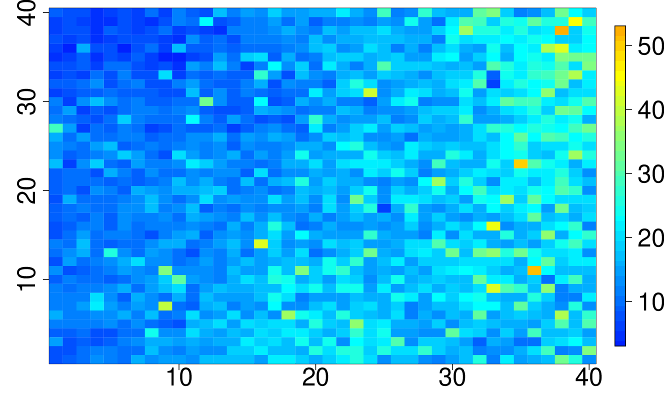

The advantage of the max-stable hierarchical model over the conditional independence model is that the former can account for local dependence; even with only 50 locations in the region, it seems to be able to detect the true pattern of local dependence. The 95% credible intervals for the elements , and of are , and , which include the true values 6, 0, and 6. The fitted max-stable model provides a mechanism for producing realistic draws from the spatial process. As Figure 7 shows, a draw from the posterior distribution of the conditional independence model would be inappropriate and unrealistic for spatial phenomena such as rainfall or temperature, annual maxima of which would produce smoother surfaces.
These results are obtained from a (near) perfect model simulation; that is, the max-stable hierarchical model fitted to the data was nearly identical to that from which the data were simulated. Nevertheless, this simulation exercise shows that the adjusted max-stable hierarchical model can flexibly model marginal behavior that captures regional spatial effects and can capture local dependence through the max-stable process model. Despite the approximation due to employing a composite likelihood, the inference obtained appropriately captures the uncertainty associated with the estimation. In the next section we show that it also seems to perform well on real data.
5 Application

We analyze data on maximum daily rainfall amounts for the years 1962–2008 at 51 sites in the Plateau region of Switzerland; see Figure 8. The area under study is relatively flat, the altitudes of the sites varying from 322 to 910 meters above mean sea level. Data from 16 of the stations were were kept aside for model validation and not used for fitting.

Figure 9 compares the annual maxima over the validation stations, which we term the “groupwise maxima”, and the simulated groupwise maxima from the different models. All the max-stable based models seem able to model the distributions of the groupwise maxima, though the simple max-stable model badly overestimates the largest value, perhaps due to inaccurate trend surfaces for the GEV parameters, particularly the shape parameter. The conditional independence model shows systematic underestimation, confirming that this model is inappropriate. The unadjusted and adjusted Bayesian hierarchical models yield similar credible envelopes, which seem principally to reflect the variability of simulated conditional Gaussian processes and GEV realizations.

Figure 10 shows three simulated random fields for each model, taken from a large number of such fields. To rank these we took a disk of radius km and centered near the Zurich gauging station, and ordered the random fields according to their suprema . This allows us to summarize the intensity of a particular realization of a random field. The three rows of Figure 10 correspond to the situation where , where respectively and the level depends on the model considered. Roughly speaking, the three rows show patterns for which is expected to be exceeded once every , and years.
The conditional independence model leads to unrealistic realizations of extreme rainfall fields, but because of the deterministic trend surfaces for the marginal parameters, the simple max-stable model produces fields that are too smooth to be realistic. The unadjusted and adjusted hierarchical models seem to produce the most plausible realizations.


Figure 11 plots return level curves, i.e., graphs of the estimated th quantile of and a similar quantity for the DOB gauging station, against , and smaller disks of radius . For the smallest neighborhood, the return level curves are compared to the observations available at the Zurich and DOB gauging stations; see Figure 8.
As the neighbourhoods of radius 0.3km are very small, the return level curves should be close to the empirical curves computed from the data available at the Zurich and DOB gauging stations. This is indeed the case for Zurich, where all the models apparently reproduce the distribution of extreme rainfall quite well. The results are less convincing for the DOB gauging station where, apart from the adjusted hierarchical model, all the models seem to overestimate the largest extremes. This situation is similar to that seen in Section 4.2: the unadjusted hierarchical model produces a posterior that is too concentrated, while the max-stable trend surface model might not be flexible enough. Both models fail to capture the complicated spatial behavior of the GEV parameters.
For the neighbourhoods of radius 6km, the central panel of the figure shows a very strong discrepancy between the models, because of their different spatial assumptions. The conditional independence model yields unrealistically high return levels, of around 2m for 10-year values, for example. All the max-stable based give approximately the same return levels for return periods shorter than years. For larger return periods, the unadjusted hierarchical model gives the largest estimates. The same plots for 20 other gauging stations depicted the same patterns, suggesting that the unadjusted hierarchical model systematically overestimates the distribution of the supremum in a given neighborhood.
6 Conclusion
In this paper, motivated by a real problem in which Bayesian inference seems natural but a full likelihood is unavailable, we investigate the usefulness of composite likelihood within a Bayesian framework. The posterior distribution obtained from a naive implementation of a composite likelihood can have very poor coverage properties, owing to its inappropriate re-use of the data.
To bypass this hurdle, we propose two modifications of the composite likelihood to recover the usual asymptotic distribution of the likelihood ratio statistic at the true value of the parameters . We show how these adjustments can be implemented in Markov chain Monte Carlo algorithms and propose two ways of integrating them into the Gibbs sampler. Although the approximation degrades with distance from the parameter underlying the data, simulation studies show that the proposed framework has coverage properties similar to those obtained using the full posterior.
The work was motivated by a need to flexibly model the marginal distributions when modeling spatial extreme phenomena. We construct a Bayesian hierarchical model whose data layer is driven by a max-stable process while the marginal parameters are modeled as realizations of a stochastic process. A spatial extreme simulation study showed that this framework is able to capture complex marginal behavior as well as the spatial dependence in the data. An application to extreme rainfall around Zurich shows that the approach can capture both local dependence due to individual storms and regional dependence due to similar climatologies, thus broadening the scope of max-stable modelling beyond its current limits.
Acknowledgments
The work of M. Ribatet and A. C. Davison was supported by the CCES Extremes project, http://www.cces.ethz.ch/projects/hazri/EXTREMES. D. Cooley’s work is partly supported by National Science Foundation grant DMS-0905315.
Appendix A Asymptotic distributions of the posterior distributions
The derivation of the asymptotic normality of the posterior distribution heavily relies on Taylor expansions. Let denote the maximum composite likelihood estimate, let denote the mode of the prior distribution , and let
For large enough we have
where and .
Provided the contribution of the prior distribution vanishes as , the strong law of large numbers implies that
almost surely, and thus .
The derivation of the asymptotic distribution for the magnitude adjustment uses the same argument, with a slight modification. As ,
almost surely. Since is estimated prior to running the MCMC algorithm, we can assume that is a (tuning) constant that does not depend on . Therefore the analogue of when using in place of is
almost surely, from which we conclude that .
We conclude with the derivation of the asymptotic distribution of the curvature adjusted composite likelihood. By construction we have
almost surely from which we get that
Appendix B Asymptotic variance inflation
In this appendix we argue that in many cases in which the densities appearing in the composite likelihood are correct, so that they satisfy the first two Bartlett identities, and for all , then . This agrees with our empirical experience, which is that in many cases .
We first note that
Since is positive semi-definite, the result follows if is positive semi-definite, because when both and are positive semi-definite.
On the one hand we have
because the variance of the score equals the Fisher information for each individual summand. On the other hand we have
Thus
say; clearly these expectations are symmetric. To see that they will often be positive definite, let and correspond to the events and . If these events are independent, then , but if not, suppose that that we may write let , , for some event such that and are independent conditional on . This arises if, for example, in a Markov chain corresponds to , corresponds to , and we take , and . If we write , then the corresponding log likelihood derivative may be written as in a natural notation, and
because the cross terms , as may be seen by conditioning on . If and are independent conditional on , then is positive semi-definite; this would be the case in the Markov chain example mentioned above. If they are not independent, but are sufficiently weakly correlated conditional on that the term is dominant, then will also be positive semi-definite, and hence so will be . This will be the case in typical applications of composite likelihood, as terms that correspond to dependent events will tend to be positively correlated, because they are proximate in space or time, or both.
References
- Chandler and Bate, [2007] Chandler, R. E. and Bate, S. (2007). Inference for clustered data using the independence loglikelihood. Biometrika, 94(1):167–183.
- Chang and Mukerjee, [2006] Chang, I. H. and Mukerjee, R. (2006). Probability matching property of adjusted likelihoods. Statistics & Probability Letters, 76(8):838–842.
- Cooley et al., [2007] Cooley, D., Nychka, D., and Naveau, P. (2007). Bayesian spatial modeling of extreme precipitation return levels. J. Am. Stat. Assoc., 102(479):824–840.
- Copas, [1972] Copas, J. B. (1972). The likelihood surface in the linear functional relationship problem. Journal of the Royal Statistical Society series B, 34:274–278.
- Davison, [2003] Davison, A. (2003). Statistical Models. Cambridge Series in Statistical and Probabilistic Mathematics. Cambridge University Press.
- de Haan, [1984] de Haan, L. (1984). A spectral representation for max-stable processes. The Annals of Probability, 12(4):1194–1204.
- de Haan and Pereira, [2006] de Haan, L. and Pereira, T. T. (2006). Spatial extremes: Models for the stationary case. The Annals of Statistics, 34:146–168.
- Efron, [1993] Efron, B. (1993). Bayes and likelihood calculations from confidence intervals. Biometrika, 80(1):3–26.
- Genton et al., [2011] Genton, M. G., Ma, Y., and Sang, H. (2011). On the likelihood function of Gaussian max-stable processes. Biometrika, 98:To appear.
- Gholamrezaee, [2010] Gholamrezaee, M. M. (2010). Geostatistics of Extremes: A composite likelihood approach. PhD thesis, École Polytechnique Fédérale de Lausanne.
- Kabluchko et al., [2009] Kabluchko, Z., Schlather, M., and de Haan, L. (2009). Stationary max-stable fields associated to negative definite functions. Ann. Prob., 37(5):2042–2065.
- Kent, [1982] Kent, J. T. (1982). Robust properties of likelihood ratio tests. Biometrika, 69:19–27.
- Lazar, [2003] Lazar, N. A. (2003). Bayesian empirical likelihood. Biometrika, 90(2):319–326.
- Lindsay, [1988] Lindsay, B. (1988). Composite likelihood methods. Statistical Inference from Stochastic Processes. American Mathematical Society, Providence.
- Monahan and Boos, [1992] Monahan, J. and Boos, D. (1992). Proper likelihoods for Bayesian analysis. Biometrika, 79(2):271–278.
- Padoan et al., [2010] Padoan, S., Ribatet, M., and Sisson, S. (2010). Likelihood-based inference for max-stable processes. Journal of the American Statistical Association (Theory & Methods), 105(489):263–277.
- Pauli et al., [2011] Pauli, F., Racugno, W., and Ventura, L. (2011). Bayesian composite marginal likelihoods. Statistica Sinica, 21:149–164.
- Robert and Casella, [2005] Robert, C. P. and Casella, G. (2005). Monte Carlo Statistical Methods (Springer Texts in Statistics). Springer-Verlag New York, Inc., Secausus, NJ, USA.
- Rotnitzky and Jewell, [1990] Rotnitzky, A. and Jewell, N. (1990). Hypothesis testing of regression parameters in semiparametric generalized linear models for cluster correlated data. Biometrika, 77:495–497.
- Rue and Tjelmeland, [2002] Rue, H. and Tjelmeland, H. (2002). Fitting gaussian markov random fields to gaussian fields. Scandinavian Journal Of Statistics, 29(1):31–49.
- Rydén and Titterington, [1998] Rydén, T. and Titterington, D. M. (1998). Computational Bayesian analysis of hidden Markov models. Journal of Computational and Graphical Statistics, 7(2):194–211.
- Sang and Gelfand, [2009] Sang, H. and Gelfand, A. (2009). Hierarchical modeling for extreme values observed over space and time. Environmental and Ecological Statistics, 16(3):407–426.
- Schlather, [2002] Schlather, M. (2002). Models for stationary max-stable random fields. Extremes, 5(1):33–44.
- Smith and Stephenson, [2009] Smith, E. L. and Stephenson, A. G. (2009). An extended Gaussian max-stable process model for spatial extremes. Journal of Statistical Planning and Inference, 139:1266–1275.
- Smith, [1990] Smith, R. L. (1990). Max-stable processes and spatial extreme. Unpublished manuscript.
- Varin, [2008] Varin, C. (2008). On composite marginal likelihoods. AStA Advances in Statistical Analysis, 92(1):1–28.
- Ventura et al., [2009] Ventura, L., Cabras, S., and Racugno, W. (2009). Prior distributions from pseudo-likelihoods in the presence of nuisance parameters. Journal of the American Statistical Association, 104(486):768–774.