The WiggleZ Dark Energy Survey: Direct constraints on blue galaxy intrinsic alignments at intermediate redshifts
Abstract
Correlations between the intrinsic shapes of galaxy pairs, and between the intrinsic shapes of galaxies and the large-scale density field, may be induced by tidal fields. These correlations, which have been detected at low redshifts () for bright red galaxies in the Sloan Digital Sky Survey (SDSS), and for which upper limits exist for blue galaxies at , provide a window into galaxy formation and evolution, and are also an important contaminant for current and future weak lensing surveys. Measurements of these alignments at intermediate redshifts () that are more relevant for cosmic shear observations are very important for understanding the origin and redshift evolution of these alignments, and for minimising their impact on weak lensing measurements. We present the first such intermediate-redshift measurement for blue galaxies, using galaxy shape measurements from SDSS and spectroscopic redshifts from the WiggleZ Dark Energy Survey. Our null detection allows us to place upper limits on the contamination of weak lensing measurements by blue galaxy intrinsic alignments that, for the first time, do not require significant model-dependent extrapolation from the SDSS observations. Also, combining the SDSS and WiggleZ constraints gives us a long redshift baseline with which to constrain intrinsic alignment models and contamination of the cosmic shear power spectrum. Assuming that the alignments can be explained by linear alignment with the smoothed local density field, we find that a measurement of in a blue-galaxy dominated, CFHTLS-like survey would be contaminated by at most (95 per cent confidence level, SDSS and WiggleZ) or (WiggleZ alone) due to intrinsic alignments. We also allow additional power-law redshift evolution of the intrinsic alignments, due to (for example) effects like interactions and mergers that are not included in the linear alignment model, and find that our constraints on cosmic shear contamination are not significantly weakened if the power-law index is less than . The WiggleZ sample (unlike SDSS) has a long enough redshift baseline that the data can rule out the possibility of very strong additional evolution.
Keywords:
cosmology: observations – gravitational lensing – large-scale structure of Universe – galaxies: evolution.1 Introduction
Gravitational lensing, the deflection of light due to matter between the source and the observer, is sensitive to all matter (including dark matter). As a result, in the past decade, weak gravitational lensing (Bartelmann & Schneider, 2001; Refregier, 2003) has become a powerful tool for addressing outstanding questions related to cosmology and galaxy formation. Its scientific applications include measurement of the amplitude of matter fluctuations using the auto-correlation of galaxy shapes (Hoekstra et al., 2006; Semboloni et al., 2006; Benjamin et al., 2007; Massey et al., 2007b; Schrabback et al., 2009, e.g., most recently, ), known as cosmic shear; and determination of the relationship between the baryonic content and the dark matter content of galaxies, using the cross-correlation between background galaxy shapes and foreground galaxy positions (Hoekstra et al., 2005; Heymans et al., 2006a; Mandelbaum et al., 2006c, e.g., ), known as galaxy-galaxy lensing. Because of the utility of these applications of lensing, plus its potential to constrain models of dark energy by splitting the sample of source galaxies into redshift slices (Hu, 2002; Huterer, 2002, tomography: ), future surveys are being planned to measure the lensing signal with sub-per cent statistical errors.
There is a large body of work devoted to solving the technical problems in measuring the weak lensing signal, primarily related to unbiased shear estimation (Heymans et al., 2006b; Massey et al., 2007a; Bridle et al., 2009) and to photometric redshifts (Bernstein & Jain, 2004; Ishak & Hirata, 2005; Huterer et al., 2006; Abdalla et al., 2008). In this work, we focus on a source of astrophysical uncertainty, intrinsic alignments of galaxy shapes. When measuring the lensing signal, it is assumed that in the absence of lensing, galaxy shapes are uncorrelated. Intrinsic alignments are alignments of galaxy shapes that violate that assumption, for example due to the alignment of galaxy shapes with a local tidal field. These alignments can therefore contaminate the gravitational lensing signal.
One type of intrinsic alignment is the correlation between the intrinsic ellipticities of two galaxies (II correlations) that reside in the same local or large-scale structure. Cosmological -body simulations robustly predict alignments between the shapes of dark matter halos that are a declining function of separation (Splinter et al., 1997; Onuora & Thomas, 2000; Faltenbacher et al., 2002; Hopkins et al., 2005; Lee et al., 2008). However, the true observational impact of these alignments are difficult to estimate using -body simulations, because the observed alignments depend on the shape of the baryonic component of the galaxy rather than on dark matter alone. While several analytical models for these alignments have also been developed (Croft & Metzler, 2000; Heavens et al., 2000; Catelan et al., 2001; Crittenden et al., 2001; Jing, 2002), they predict wildly varying levels of alignment, so observational constraints are necessary.
More recently, Hirata & Seljak (2004) pointed out that the correlation of galaxy shapes with large-scale density fields can also contaminate lensing measurements. These alignments, known as GI correlations, are caused by a lower redshift tidal field that both causes gravitational shear experienced by a higher redshift galaxy, and intrinsically aligns the shape of galaxies that are in the tidal field. GI correlations are also predicted to have very different magnitudes depending on the model used to estimate them (Hui & Zhang, 2002; Hirata & Seljak, 2004; Heymans et al., 2006c), and have been detected using dark matter halos at many different mass scales in -body simulations (Bailin & Steinmetz, 2005; Altay et al., 2006; Basilakos et al., 2006; Heymans et al., 2006c; Kuhlen et al., 2007).
The relevant signature of these GI correlation detections in -body simulations is that dark matter halos align so that they point preferentially towards other halos that are part of the same large-scale structure. When considering GI correlations of galaxies that contaminate cosmological weak lensing measurements, the effect is manifested as galaxy shapes that point preferentially towards other galaxies (both locally, within a halo, and on cosmological scales). These alignments of galaxy shapes are anti-correlated with the gravitational shear due to large-scale structure, so GI correlations reduce the measured cosmic shear signal, unlike the II correlations which increase it. Also unlike the II correlations, the GI correlations are not due to the inclusion of galaxy pairs at the same redshift; pairs at different redshifts are affected when the higher redshift galaxy of the pair is lensed by a structure that has caused an intrinsic alignment of the lower redshift galaxy.
Several different schemes have been proposed to remove intrinsic alignment contamination from weak lensing measurements, including the removal of galaxy pairs that are close in redshift space (to remove II: King & Schneider 2002; King & Schneider 2003; Heymans & Heavens 2003; Takada & White 2004); projecting out both types of intrinsic alignments using their known scalings with the redshifts of the galaxy pair (Hirata & Seljak, 2004; Joachimi & Schneider, 2008; Zhang, 2008; Joachimi & Schneider, 2009); and modeling them jointly with the lensing signal using some parametric models, the parameters of which are then marginalised over (King, 2005; Bridle & King, 2007). A common feature of these methods is a loss of information, and therefore weakening of cosmological constraints from the weak lensing signal. Measurements of intrinsic alignments can place strong priors on the intrinsic alignment model, which would minimise the loss of cosmological information from future surveys. Direct intrinsic alignment measurements will also constrain the impact of intrinsic alignments on previous lensing measurements that did not explicitly account for them. This measurement is particularly important given the aforementioned difficulty in theoretical predictions; however, the observations can then be used to refine the theory and, in turn, learn something about galaxy formation and evolution.
To observe intrinsic alignments, we require a source of data with robust galaxy shape measurements free of contamination from the PSF, and a way of isolating nearby (in all three dimensions) galaxy pairs. The GI correlations are then measured by calculating, statistically, the tendency for galaxies to point towards other galaxies that are relatively nearby (on tens of Mpc scales). Alternatively, it is possible to measure II correlations at low redshift without any redshift information, given that the cosmic shear signal below is vanishingly small (Brown et al., 2002). On the large scales used for cosmological lensing analyses, the first measurement of GI correlations used SDSS data (Mandelbaum et al., 2006b), with a follow-up analysis by Hirata et al. (2007) that also included redshifts of SDSS Luminous Red Galaxies (LRGs) and from the 2dF-SDSS LRG and QSO survey (2SLAQ, Cannon et al. 2006) to constrain intrinsic alignments of red galaxies up to intermediate redshifts, –. While GI correlations were detected in these works at – for bright red galaxies (and II correlations for the same galaxy sample were found by Okumura et al. 2009), with a weak () detection at intermediate redshifts (due to the small size of the 2SLAQ sample), further work at intermediate to high redshift is crucial for constraining the impact of intrinsic alignments on cosmological lensing analyses. It is difficult to extrapolate these low-redshift analyses to higher redshift, because different dynamical scenarios might entail very different redshift evolution. For example, blue galaxies at that have no measurable GI alignment in SDSS may have been very highly aligned with the density field at intermediate-high redshift, with mergers and interactions serving to disrupt those alignments, leading to the null detection that we see at low redshift; or, these alignments might be very small at all redshifts.
Due to its overlap with the SDSS, which provides galaxy shape measurements, the WiggleZ Dark Energy survey (Drinkwater et al., 2010) is an ideal source of spectroscopic redshifts for constraining intrinsic alignments of UV-selected blue galaxies at intermediate redshift. In this work, we use that sample to attempt the first measurement of galaxy intrinsic alignments for blue galaxies at intermediate redshift, which fills in a very important gap in our knowledge of intrinsic alignments. At higher redshift, we expect that blue galaxies will dominate the galaxy samples used for weak lensing. Thus, these observations will facilitate further development in the fields of weak lensing and galaxy dynamics and evolution.
Here we note the cosmological model and units used throughout this work. Pair separations are measured in comoving Mpc (where km sMpc-1), with the angular diameter distance computed in a spatially flat CDM cosmology with . For the bias and cosmic shear calculations, we additionally normalise the matter power spectrum using , set the baryon density and scalar primordial spectral index , and use the transfer function from Ma (1996).
We begin in Section 2 with a summary of the intrinsic alignment and cosmic shear formalism used in this work. Section 3 contains descriptions of data used for the analysis. The methodology used for the data analysis is described in Section 4. We present the results of the analysis in Section 5, including systematics tests and a comparison with previous observations. The interpretation of these results, including an estimate of contamination of the cosmic shear signal, is given in Section 6, and we conclude in Section 7.
2 Formalism
Here we briefly summarise the formalism for the analysis of intrinsic alignment contamination to the lensing shear correlation function. Our notation is consistent with that of Hirata & Seljak (2004), Mandelbaum et al. (2006b), and Hirata et al. (2007).
The observed shear of a galaxy is a sum of two components: the gravitational lensing-induced shear , and the “intrinsic shear” , which includes any non-lensing shear, typically due to local tidal fields. Therefore we can write the -mode shear power spectrum between any two redshift bins and as the sum of the gravitational lensing power spectrum (GG), the intrinsic-intrinsic, and the gravitational-intrinsic terms,
| (1) |
Mandelbaum et al. (2006b) presented the Limber integrals that allow us to determine each of these quantities in terms of the matter power spectrum and intrinsic alignments power spectrum. In a flat universe, the GI contamination term can be written as
| (2) | |||||
where is the comoving distance to the horizon, is the comoving distance distribution of the galaxies in sample , and
| (3) |
The generalisation of these equations to curved universes can be found in Mandelbaum et al. 2006b.
The density-intrinsic shear cross-power spectrum that enters into Eq. (2) is defined as follows. If one chooses any two points in the SDSS survey, their separation in redshift space can then be identified by the transverse separation and the radial redshift space separation . The and components of the shear are measured with respect to the axis connecting the two galaxies (i.e., positive shear is radial, whereas negative shear is tangential). Then one can write the density-intrinsic shear correlation in Fourier space as
| (4) |
where is the correlation function between the density contrast and the galaxy density-weighted intrinsic shear, (where ). It is often convenient to do the projection along the radial direction,
| (5) |
A similar set of equations can be written for the intrinsic-intrinsic terms. For example, we can define
| (6) |
in terms of the E-mode power spectrum of the density-weighted intrinsic shear, . Likewise, the intrinsic-intrinsic correlations are
| (7) | |||||
where .
While (to first order) the lensing shear does not induce any -mode signal, intrinsic alignments are one of several effects that may contribute to a nonzero -mode power spectrum (Hirata & Seljak, 2004; Heymans et al., 2006c). However, we will not focus on these effects here.
3 Data
3.1 WiggleZ
| Sample | ||||||||
|---|---|---|---|---|---|---|---|---|
| WiggleZ all | 0.01 | 1.3 | 0.51 | -20.9 | -20.7 | 0.050 | 0.33 | |
| WiggleZ | 0.01 | 0.52 | 0.37 | -19.9 | -19.4 | 0.032 | 0.34 | |
| WiggleZ | 0.52 | 1.3 | 0.62 | -21.2 | -21.0 | 0.064 | 0.32 | |
| SDSS Blue L4 | 0.02 | 0.19 | 0.09 | -20.8 | -20.8 |
The WiggleZ Dark Energy Survey at the Anglo-Australian Telescope (Drinkwater et al., 2010) is a large-scale galaxy redshift survey of bright emission-line galaxies mapping a volume of order 1 Gpc3 over the redshift range . The survey, which began in August 2006 and is scheduled to finish in July 2010, is obtaining redshifts for UV-selected galaxies covering deg2 of equatorial sky. It is performed using the multi-fibre spectrograph AAOmega, which can simultaneously obtain spectra for up to 392 galaxies over a 2-degree-diameter field-of-view (Sharp et al., 2006). The principal scientific goal is to measure the baryon acoustic oscillation signature in the galaxy power spectrum at a significantly higher redshift than existing surveys. The target galaxy population is selected from UV imaging by the Galaxy Evolution Explorer (GALEX) satellite, matched with optical data from the Sloan Digital Sky Survey (SDSS) and Red Cluster Sequence survey (RCS2) to provide accurate positions for fibre spectroscopy.
In this paper, we analyse the subset of the WiggleZ sample lying in the SDSS survey areas assembled up to the end of the 09A semester (May 2009). Specifically, we include data from the WiggleZ 9-hr (09h), 11-hr (11h), and 15-hr (15h) regions, centred at the following positions: , , and respectively (all positions are in degrees of right ascension and declination, J2000 equatorial coordinates). These regions together include 76 084 galaxies with spectroscopic redshifts classified as reliable (with quality , see Drinkwater et al. 2010), with the three regions containing 22 011, 21 746, and 32 327 galaxies, respectively. The number density of galaxies with successful redshift estimates varies within these regions from to per square degree, depending on how completely a given region was observed. These galaxies constitute an extended sample relative to the one used for the analysis in Blake et al. (2009). As a consequence of the continuing GALEX imaging campaign in the WiggleZ survey regions, the UV magnitudes of a fraction of the targets have been refined as the survey progresses, causing some originally-observed galaxies to now fail the survey magnitude and colour selection cuts. This subset of galaxies was not included in the original clustering analysis of Blake et al. (2009), but has now been accommodated following suitable modifications to the random catalogue generation procedure. Full details will be presented in a future paper.
The redshift error rate for galaxies that are assigned a redshift, which is a function of redshift, is given in Table 1. As shown in Blake et al. (2009) figure 13, the typical -band luminosity of this sample ranges from two magnitudes below at , to at , to two magnitudes above at . For simpler comparison against SDSS, Table 1 shows the rest-frame -band magnitudes for this sample. These were derived on average from the UV and band photometry, using a Lyman Break Galaxy template that is consistent with the WiggleZ galaxies being detected in the near-UV (NUV) but being far-UV dropouts. This template is a constant star formation rate model, with significant dust extinction added to match the observed NUV- colour versus redshift relation. Figure 3 of Wyder et al. (2007), which shows the NUV- colour-magnitude relation for galaxies with measurements from GALEX and SDSS around , is a good illustration of the nature of the WiggleZ sample. That figure shows a distinct, well-defined red sequence and a blue cloud, where the WiggleZ selection of NUV- picks out the very blue edge of the blue cloud.
We create random catalogues for each WiggleZ region using the method described by Blake et al. (2009) with modifications to account for the use of an extended sample. In brief, random realisations of “parent” catalogues are first created which trace the variation in WiggleZ target density with Galactic dust extinction and GALEX exposure time. These realisations are then processed into random “redshift” catalogues by imposing the observing sequence of telescope pointings. The fraction of successful redshifts in each pointing varies considerably depending on weather conditions. Furthermore, the redshift completeness within each pointing exhibits a significant radial variation due to acquisition errors at the plate edges, which is also modelled.
In order to model the observed intrinsic alignment signal, we require a measurement of the bias of the sample used to trace the density field, which is the full WiggleZ redshift sample (including those galaxies without shape measurements). The galaxy biases that we use for this analysis were measured using the method of Blake et al. (2009), which (in brief) involves the following steps: (i) measurement of the correlation function projected along the line of sight to Mpc; (ii) fitting this measurement to a power-law correlation function (also integrated along the same line-of-sight range, and with a model for redshift space distortions) to determine a correlation length; (iii) generating a dark matter correlation function using CAMB (Lewis et al., 2000) with halofit , assuming , , , , and , to determine the dark matter correlation length; and (iv) estimating a galaxy bias using the ratio of the correlation lengths, while accounting for the linear growth factor. Since we use for the cosmic shear power spectrum calculations in this paper, we also increase the Blake et al. (2009) bias measurements by so that they are consistent with this cosmological parameter choice. Finally, we correct for the effect of redshift blunders by decreasing theoretical model predictions by a factor of , which corresponds to increasing the measured correlations by .
The observed redshift distribution is, to good approximation, a double Gaussian, with 77.6 per cent of the galaxies in a Gaussian with mean and width , and the remaining 22.4 per cent in a narrower Gaussian with mean and width . We will use this description of the redshift distribution in our theoretical modeling of the observations.
3.2 SDSS spectroscopic sample
In this paper, we compare the WiggleZ results with previous measurements of intrinsic alignments using a sample of SDSS spectroscopic galaxies that are blue and have luminosities near , the “blue L4” sample from Hirata et al. (2007). The properties of this sample are also given in Table 1. In that paper, we were interested in robustly isolating the red sequence from the blue cloud, so the colour separator used there defined this “blue” sample to include the entire blue cloud. The -band luminosities used to define this sample were -corrected to using kcorrect v3_2 (Blanton et al., 2003) with Petrosian apparent magnitudes, extinction corrected using the reddening maps of Schlegel et al. (1998) and extinction-to-reddening ratios from Stoughton et al. (2002). For fair comparison with the WiggleZ sample, here we calculate luminosities with the model magnitudes, and correct to .
3.3 Galaxy shape measurements
For a subset of the WiggleZ galaxies, we use shape measurements from the SDSS. The SDSS (York et al., 2000) imaged roughly steradians of the sky, and followed up approximately one million of the detected objects spectroscopically (Eisenstein et al., 2001; Richards et al., 2002; Strauss et al., 2002). The imaging was carried out by drift-scanning the sky in photometric conditions (Hogg et al., 2001; Ivezić et al., 2004), in five bands () (Fukugita et al., 1996; Smith et al., 2002) using a specially-designed wide-field camera (Gunn et al., 1998). These imaging data were used to create the galaxy shape measurements that we use in this paper. All of the data were processed by completely automated pipelines that detect and measure photometric properties of objects, and astrometrically calibrate the data (Lupton et al., 2001; Pier et al., 2003; Tucker et al., 2006). The SDSS has had seven major data releases, and is now complete (Stoughton et al., 2002; Abazajian et al., 2003; Abazajian et al., 2004; Abazajian et al., 2005; Finkbeiner et al., 2004; Adelman-McCarthy et al., 2006; Adelman-McCarthy et al., 2007; Adelman-McCarthy et al., 2008; Abazajian et al., 2009).
We use the galaxy ellipticity measurements by Mandelbaum et al. (2005), who obtained shapes for more than 30 million galaxies in the SDSS imaging data down to extinction-corrected magnitude using the Reglens pipeline. We refer the interested reader to Hirata & Seljak (2003) for an outline of the PSF correction technique (re-Gaussianization) and to Mandelbaum et al. (2005) for all details of the shape measurement. The full details of restrictions imposed on galaxy shape measurements are in Mandelbaum et al. (2005), but the two main criteria for the shape measurement to be considered high quality are that galaxies must (a) have extinction-corrected -band model magnitude , and (b) be well-resolved compared to the PSF size in both and bands (as quantified by the adaptive moments of the PSF and galaxy image). The WiggleZ galaxies with shape measurements were part of the general SDSS shape catalog presented in Mandelbaum et al. (2005) and used for many subsequent science papers. Thus, they have already been subjected to all systematics tests detailed in those papers, particularly the original paper and Mandelbaum et al. (2006a), which has other significant tests of shear systematics. Nonetheless, in this paper we will still present additional systematics tests to rule out the possibility that this sample has some unusual set of systematics compared to the rest of the shape catalog.
In the 09h, 11h, and 15h fields, the fractions of WiggleZ galaxies with high-quality shape measurements are 33, 34, and 32 per cent, respectively, giving a number density that ranges from 60 to 100 degree-2. Figure 1 shows the redshift and -band model magnitude distributions for the WiggleZ redshift sample, and the fraction with good shape measurements. As shown, the probability that there is a good shape measurement exhibits a significant magnitude dependence, and goes to zero for due to a cut imposed on the shape catalogue. However, the redshift distribution of those galaxies with shapes is not substantially different from that of the full sample, because at any given redshift the most luminous galaxies tend to be large enough in apparent size relative to the PSF that they have a measurable shape. There is also a slight region-to-region variation of the match fraction, for two main reasons: because the typical seeing in the SDSS observations varies with position, and because the pointing strategy of the WiggleZ observations prioritises fainter galaxies, which are less likely to have a good shape measurement, so the more completely observed regions will tend to have a higher match fraction.

To do this measurement, we also need random catalogues that correspond to the shape-selected subset of the galaxies. To flag a fraction of galaxies in our random galaxies as possessing “good shapes,” we estimated (from the data) the probability of a galaxy possessing a good shape as a function of the seeing of the SDSS observation and of the galaxy magnitude, and imposed this probability function on the random points (separately in each region). As shown in Fig. 1, the good shape fraction is a decreasing function of magnitude; as expected, we find that it is also a decreasing function of the seeing FWHM.
4 Methodology
The software for computation of correlation functions is the same as that used in Mandelbaum et al. (2006b) and Hirata et al. (2007). In order to find pairs of galaxies, this code uses the SDSSpix package.11 1 http://lahmu.phyast.pitt.edu/˜scranton/SDSSPix/ To reduce noise in the determination of galaxy-random pairs, we use 100 random points for each real galaxy in the catalogue. The correlation functions are computed over a 120 Mpc (comoving) range along the line of sight from to Mpc, divided into 24 bins with size Mpc, and the projected correlation function is computed by “integration” (technically summation of the correlation function multiplied by ) over . This value of was chosen to minimise the loss of correlated galaxy pairs at all projected separations used here (Padmanabhan et al., 2007) without increasing the noise excessively. We also show results with Mpc, which have better but are more complicated to interpret due to redshift space distortions, and therefore are not used for cosmological interpretation in this paper.
This calculation is done in radial bins from Mpc. Covariance matrices are determined using a jackknife with 49 regions, in order to account properly for shape noise, shape measurement errors, and cosmic variance. This number was chosen to be large enough to obtain a stable covariance matrix for the fits (it must be larger than ; see Appendix D of Hirata et al. 2004) but small enough that the size of a given jackknife region is larger than the scale on which the correlation is to be measured. Each such calculation is carried out separately for the three WiggleZ regions, to check for consistency, before averaging over the regions.
The code measures several different correlation functions simultaneously; here we describe the estimator for each one.
For the GI cross-correlation function , we use a generalisation of the LS (Landy & Szalay, 1993) estimator for the galaxy correlation function. This generalisation can be expressed as
| (8) |
where is the sum over all real (“data”) galaxy pairs (with one galaxy in the subset with shapes, and the other galaxy in the full WiggleZ redshift sample) with separations and of the component of shear:
| (9) |
where is the component of the ellipticity of shape sample galaxy measured relative to the direction to density field galaxy , and is the shear responsivity (that represents the response of our ellipticity definition to a small shear; Kaiser et al. 1995, Bernstein & Jarvis 2002). is defined by a similar equation, but using pairs derived from the real sample with shape measurements and the full random catalogues. is the number of pairs of random galaxies with separations and such that one of those random galaxies is in the subset that is statistically likely to have a good shape measurement in SDSS, and the other is in the full WiggleZ random sample. ( and are understood to be rescaled appropriately since the number of random catalogue galaxies differs from the number of data galaxies.) Note that when doing the summation in Eq. (9) to determine (or the comparable summations for and ), we use all pairs regardless of which galaxy, or (in the density field tracer and intrinsic shear tracer samples, respectively), is in the foreground. The reason for this choice is that we are attempting to detect an alignment due to the two galaxies experiencing the same tidal field since they are in close 3D proximity, rather than a lensing effect (which would require them to be at different redshifts).
Averaged over a statistical ensemble, , so that systematics in the shear or the number density cancel to first order. Positive indicates a tendency to point towards over-densities of galaxies (i.e., radial alignment, the opposite of the convention in galaxy-galaxy lensing that positive shear indicates tangential alignment). For the purpose of systematics tests, we can define an analogous estimator using the other (“”) ellipticity component for .
For the intrinsic shear auto-correlation functions and , we restrict ourselves to the subset of the data with shape measurements, and use the estimators
| (10) |
where
| (11) |
(with both and denoting galaxies in the shape-selected sample) and similarly for . Since , the cancellation of systematics to first order works again, i.e. the square of any spurious source of shear adds to Eq. (10) instead of the shear itself. Projected quantities such as and are then obtained by line-of-sight integration.
Note that the intrinsic shear autocorrelation, , may potentially have some contribution from cosmic shear. However, for the median redshift of the WiggleZ sample, the predicted contribution from cosmic shear to (for a concordance cosmology) is of order at 10 Mpc (see, for example, Jarvis et al. 2006; to estimate the cosmic shear contribution to we must include a factor of due to the line-of-sight integration). We shall see in Section 5 that this cosmic shear contribution is well below our errorbars and therefore undetectable. This is a consequence of the very low galaxy number density for the subset of the WiggleZ sample that has good shape measurements, which means that a cosmic shear measurement is not feasible (even were we to avoid the restriction that the pairs be close along the line-of-sight, which is necessary to detect intrinsic alignments, but not cosmic shear).
5 Results
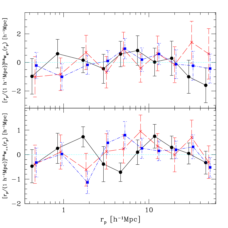
We begin by presenting the projected intrinsic alignment cross-correlation functions, and . The results are shown for each region in Fig. 2. We have scaled the signal by for easy viewing. As shown, both and are consistent with zero in all regions. Furthermore, there is no sign of any systematic discrepancy between the results in different regions, so for all subsequent tests we present only the results averaged over region (shown in Fig. 4). Adjacent radial bins on large scales are correlated at the level of several tens of per cent for , whereas is sufficiently dominated by shape noise that the points are nearly uncorrelated.
As shown in Fig. 2, the errorbars for and are within a factor of two of each other. It is worth considering at this point what value the measurement has for constraining intrinsic alignments. As shown in Hirata & Seljak (2004), the linear alignment model at predicts that for typical scales used in this measurement, the ratio of the II to the GI power spectra is of order . Thus, within the context of the linear alignment model, our non-detection of GI alignments implies an even lower II amplitude that, given our errorbars, will be undetectable. We can conclude that the non-detection of II does not give us significant additional information about intrinsic alignments within the context of the linear alignment model. The utility of our II measurement is that it allows us to (a) rule out significant shear systematics that would lead to galaxy shape correlations significant enough that they might affect , and (b) rule out substantial intrinsic alignments due to other causes besides the linear alignment model. For example, the simplest form of the quadratic alignment model (Catelan et al., 2001; Hui & Zhang, 2002; Hirata & Seljak, 2004) predicts zero GI-type alignments, but nonzero II alignments.
To assess the consistency of these signals with zero, we include Table 2. This table shows the for a fit to zero signal, including correlations between radial bins (by using the full inverse covariance matrix). We also include the probability for a random vector with this covariance matrix to exceed the given by chance, . To calculate this probability value, we included the fact that the jackknife covariance matrices lead to a value that does not follow the expected distribution, because of noise from the finite number of jackknife regions. To include the effects of noise, we use a simulation based on the formalism in Appendix D of Hirata et al. (2004). As shown in the first two lines of Table 2, the and shown in Fig. 2 are indeed consistent with zero, given that our criterion for inconsistency with zero is .
| range | range | statistic | ||
|---|---|---|---|---|
| ( Mpc) | ||||
| All | 4.83 | 0.90 | ||
| All | 14.53 | 0.25 | ||
| 8.98 | 0.60 | |||
| 13.28 | 0.30 | |||
| 7.24 | 0.84 | |||
| 18.08 | 0.13 | |||
| All | 15.82 | 0.20 | ||
| All | 14.92 | 0.23 | ||
| All | 3.67 | 0.96 | ||
| All | 18.21 | 0.13 | ||
| All | 8.60 | 0.62 | ||
| All | 8.70 | 0.62 | ||
| All | 5.60 | 0.85 |
Next, we split the galaxies at and recompute these correlation functions for each redshift subsample, with effective redshifts of and , respectively (see Table 1). This value of redshift was chosen to give approximately of the galaxies at , and 2/3 above, which (given the higher measurement noise in the latter sample) yields approximately equal for the and measurements in the two redshift slices. As shown in Blake et al. (2009) and our Table 1, this split corresponds to a luminosity split. Fig. 3 shows that the results for the two redshift slices are consistent with each other, with no detection of any intrinsic alignment signal. These null results can also be confirmed using the third through sixth lines of Table 2.

Finally, in Fig. 4 we show the results with the two different values of , and Mpc. As previously noted, the former results (while less noisy) are more complex to interpret due to the need for a model of redshift-space distortions, and so we use the latter for all cosmological interpretation. However, we can confirm again in lines 7 and 8 of Table 2 that the results with the smaller value are also consistent with zero.

5.1 Systematics tests
In this section we present several systematics tests, though the galaxy shape measurements used for this paper were already tested extensively in Mandelbaum et al. (2005) and subsequent papers. While these tests may seem irrelevant given the null results for and , we would like to rule out the possibility that a real astrophysical signal may be masked by a systematic error of similar magnitude but opposite sign. We also, however, note that the most likely sign of contributions of both PSF systematics and intrinsic alignments to is positive, so the null detection itself constitutes a constraint on systematics.
The first test involves the use of the other ellipticity component to compute and (which should be zero by symmetry for a real astrophysical signal, since intrinsic alignments only induce alignments in the radial/tangential direction, but may be generated due to certain errors in PSF correction). As shown in Fig. 5, there is no sign of either of these signals; they are completely consistent with zero, as confirmed in Table 2.

The second systematics test is to compute these signals using pairs at large line of sight separations, Mpc. This test will help show whether there is any spurious signal due to some systematic effect, since those pairs are effectively not correlated. Figure 6 shows no sign of nonzero or for pairs at large line-of-sight separations, indicating that the potential contaminants to the signal are within the errors. Table 2 confirms this finding quantitatively.

5.2 Comparison with previous observations
There have been several previous measurements of large-scale intrinsic alignments. We focus on those that are presented using comparable estimators that include the ellipticity (i.e., not those that correlate the position angles) and on those that go to the large scales that are of interest for cosmic shear.
First, Mandelbaum et al. (2006b) presented GI and II correlations for SDSS Main spectroscopic sample galaxies (typical ) split into luminosity bins, which included a positive detection of GI signal for the bins with . Next, Hirata et al. (2007) showed results for the Main sample split into both colour and luminosity bins, in addition to new results from the SDSS LRG sample (red galaxies with ) and from the 2SLAQ redshift survey using shape measurements from SDSS.
On Fig. 7, we show the measured for the WiggleZ sample, for one of the four blue galaxy samples derived from the SDSS Main galaxy sample (L4, with ); for the intermediate SDSS LRG luminosity bin in Hirata et al. (2007); and for the 2SLAQ sample (a red galaxy sample at the same typical redshift as WiggleZ, Cannon et al. 2006).

As shown in this figure, the signals for “typical” blue galaxies at (SDSS blue L4), and for UV-selected galaxies at (WiggleZ) are consistent with zero. The constraints are tighter using SDSS than using WiggleZ despite the larger volume of the WiggleZ survey, because the WiggleZ survey is shot-noise limited on small scales given the sparse sampling of the galaxies that are targeted for spectroscopy. However, the WiggleZ measurement is the first at cosmologically relevant redshifts for blue galaxies, which tend to dominate cosmic shear samples.
Detailed comparison of the SDSS blue L4 sample and WiggleZ sample is difficult, but Table 1 suggests that they have similar rest-frame -band absolute magnitudes. Given that typically tends to get brighter with redshift (Wolf et al., 2003, e.g., ), this suggests that the WiggleZ galaxies are in fact fainter relative to in -band than the SDSS sample. However, Wyder et al. (2007) show that the WiggleZ galaxies occupy the very blue edge of the blue cloud, so the fact that both samples are blue does not necessarily imply comparable similar formation and evolution scenarios. With this caveat, if we naively combine the two results, we can show that the GI correlations are not significant for blue galaxies over a large range of redshifts; we will quantify this statement and its cosmological implications in Sec. 6. Even if this combination of the two samples is not valid, the WiggleZ result is highly useful because of its proximity to redshifts used for cosmic shear studies.
The constraints with the 2SLAQ sample, originally presented and interpreted in Hirata et al. (2007), give a slight suggestion of nonzero GI alignments at the level. (For reference, we also show the strong positive detection for one of several SDSS LRG luminosity bins, which has a higher mean luminosity and lower mean redshift.) In contrast with the results for red galaxies, the WiggleZ galaxies at the same redshift have no such suggestion of nonzero signal, and the constraints are significantly tighter because the sample size is larger.
Finally, we present a comparison against the results of Heymans et al. (2006c), who use -body simulations to investigate the intrinsic alignment signals resulting from different methods of populating the dark matter halos with galaxies (including different ways of aligning the galaxy shapes with the dark matter halo or angular momentum vector). Our null result is consistent with the results for their “spiral” model, which is that of a thick disk randomly misaligned with the dark matter halo angular momentum vector. The mean misalignment angle in that model is 20∘.
6 Interpretation and cosmological implications


| Data | ||
|---|---|---|
| SDSS Main Blue L4 | ||
| WiggleZ , all | ||
| WiggleZ , all | ||
| WiggleZ , | ||
| WiggleZ , | ||
| SDSS Main Blue L4 | ||
| WiggleZ , all | ||
| WiggleZ , all | ||
| SDSS Main Blue L4 | ||
| WiggleZ , all | ||
| WiggleZ , all | ||
| WiggleZ , | ||
| WiggleZ , | ||
| SDSS Main Blue L4 | ||
| WiggleZ , all | ||
| WiggleZ , all |
We now fit two different models to our measured intrinsic alignment correlation functions, and investigate the implications of our results in terms of the bias in cosmological measurements of the amplitude of matter fluctuations from cosmic shear. In order to avoid overly optimistic constraints on model parameters due to inversion of the noisy jackknife covariance matrices, we apply the correction described by Hartlap et al. (2007) (equation 17 in that paper) after inversion. This correction compensates for the fact that the inverse of a noisy covariance matrix is not an unbiased estimate of the inverse covariance matrix, and corresponds to multiplication of the inverse covariance matrix by for 49 jackknife regions and radial bins used for the fit. Thus, for fits that only use a subset of the radial bins, we restrict to the appropriate subset of the covariance matrix, invert, and multiply by the appopriate fraction.
We first fit a power law in transverse separation to each of the measured signals, in a similar way to Mandelbaum et al. (2006b) and Hirata et al. (2007). These fits have the advantage of being very simple, and allow direct comparison with previously-published results that use the same fitting method; however, they are lacking in physical motivation. In order to give fits with physical motivation, we fit the unknown amplitude in a linear alignment model (Catelan et al., 2001; Hirata & Seljak, 2004). Using simple assumptions, these fits allow us to compare constraints from the observed correlation functions and propagate the constraints through to biases on the amplitude of matter clustering.
To interpret the observed GI correlation function in terms of the correlation between the intrinsic shape and the density field (), we assume a linear bias model and estimate the bias of the galaxies used as tracers of the density field. Values are shown in Table 1 for each of the three WiggleZ samples we consider (full sample and two redshift slices), following the methodology of Blake et al. (2009). We then assume
| (12) |
throughout. A minimum separation of Mpc is used for fits to to avoid non-linear biasing on small scales affecting the interpretation of in terms of . We use all calculated data points, with no minimum separation, when fitting to the ellipticity-ellipticity correlation function .
6.1 Power-Law Fits
We fit a power law
| (13) |
to the projected density-shape correlation function, and similarly for the II (shape-shape) correlation function . This fit is performed separately for each sample under consideration. Here is the fraction of objects with bad redshifts, as given in Table 1. We do not include a dependence on redshift in this subsection, because it would not be meaningfully constrained by any one dataset alone. We instead defer questions of redshift evolution to the following subsection.
We compute the likelihood as a function of and on a grid using , using the full covariance matrix of the data in the calculation. We used sufficiently wide ranges of and that the constraints shown are not affected. We calculate the resulting amplitudes for two cases: fixed , or marginalised over after allowing it to vary within a wide range. This fixed value for is motivated by line 5 of table 6 of H07, which gives results for SDSS LRGs using a minimum separation of Mpc. 95 per cent confidence limits were calculated by finding the iso-probability level containing 95 per cent of the probability.
The solid and dashed lines in Fig. 8 show constraints on the power law amplitude for the two line-of-sight integration ranges considered in this paper, and Mpc. As expected, the larger line-of-sight range results in a weaker constraint due to dilution of the signal by noise from uncorrelated pairs. The results from the SDSS Main Blue L4 sample (M06, H07) are shown for comparison (dot-dashed line). The SDSS results give a much tighter constraint on the amplitude of the ellipticity-ellipticity power law than the WiggleZ samples, and appear close to a delta function at on the lower panel of Fig. 8. For the ellipticity-density correlation function, the constraints from SDSS and WiggleZ are more similar. We also show the results after marginalising over the spatial power law coefficient . These results are peaked at because of the large range of values allowed if .
Fig. 9 shows the 95 per cent confidence ranges as a function of sample redshift for the SDSS data and WiggleZ redshift subsamples. Since all points are consistent with zero, there is no sign of a trend with redshift. However, a strong redshift evolution could be ruled out.
These results are summarised in Table 3 (95 per cent confidence limits). We also show results when both the amplitude and scale dependence of the power law are varied. Since the amplitude is nearly consistent with zero, the constraints on the power law slope are relatively weak and easily consistent with the fiducial value of taken from the SDSS LRG sample. We interpret the constraints as intrinsic alignments constraints, and the constraints as non-detections of both intrinsic alignments and significant shear systematics.
6.2 Linear Alignment Model Fits
We now fit a simple but physically motivated intrinsic alignment model to the observed correlation functions. We use a variant of the linear alignment model described in Catelan et al. (2001). As originally discussed in Section 5, our non-detection of GI correlations constrains the intrinsic alignments in the context of this model so that the allowed II signals are well below the size of our errors on . Thus, for this section we will only use for constraining the linear alignment model.
The linear alignment model assumes galaxies are stretched by an amount proportional to the local curvature of the smoothed gravitational potential, and was developed further by Hirata & Seljak (2004) to predict the contributions to the lensing power spectra.22 2 It has been found (Hirata 2010 in prep. and Joachimi et al 2010 in prep.) that the linear alignment model in Hirata & Seljak (2004) has an error in the derivation of its redshift evolution, and should be multiplied by a factor of . Thus, the corrected version of the linear alignment model corresponds to our zNLA model with additional redshift evolution , which as we will show in the right panel of Fig. 12 corresponds to the peak of the likelihood of (when using the combination of low-redshift SDSS data plus WiggleZ). Given that (a) this issue was discovered after these calculations were completed, (b) our constraints on are not very tight, and (c) the constraints on contamination to cosmology do not change since we integrate over a large range of , we have opted to leave all calculations and figures in terms of the Hirata & Seljak (2004) formulation of the linear alignment model. However, the reader should keep this in mind when considering our results in the context of implications for linear alignments. This model is not expected to be an accurate description of alignments on non-linear scales, and Bridle & King (2007) were inspired by H07 to insert the non-linear matter power spectrum into the model in place of the linear matter power spectrum. We refer to this model as the non-linear power spectrum linear alignment (NLA) model hereafter. A physically motivated model for smaller scales based on the halo model presented by Schneider & Bridle (2010) gives qualitatively similar results to the NLA. Note that while we use the non-linear matter power spectrum to describe the density field on small scales, we still need the linear bias assumption to relate to , and therefore cannot use very small scales when interpreting this observation (unlike for ).
We use the NLA for the rest of this Section, ignoring all but the first term in equation (16) of Hirata & Seljak (2004). It has a single free parameter, the amplitude , which is the constant of proportionality between the galaxy ellipticity and the local potential curvature. The model has an inbuilt motivated variation with scale and redshift. However, it is possible that the constant of proportionality may additionally vary with environment and galaxy type, as well as redshift. In this paper we therefore allow the amplitude of these alignments to vary with an additional free power law in redshift, with index , to include any variation with redshift due to other physics not included in the NLA model. The default value is , so that the inbuilt redshift dependence of the NLA is recovered. Our physical motivation for including this additional redshift evolution factor is to allow for more complicated effects in galaxy evolution, such as mergers and interactions. For example, a model in which galaxies align with the local tidal field at early times, but gradually decorrelate due to interactions and mergers, would be described with a positive that allows for significant alignment at early times that is not present at the current time. These models are particularly of interest since, as noted in Drinkwater et al. (2010), a significant fraction of the WiggleZ galaxies appear to be interacting, merging, or have recently undergone a merger. The full, redshift-dependent model with the power-law evolution in addition to the NLA model is called the “zNLA model.”
Thus, our model for the E-mode power spectrum of the density-weighted intrinsic shear, (Eq. 7), including this additional term is
| (14) |
Likewise, the cross-power spectrum between the intrinsic shear and density field, (Eq. 4), is
| (15) |
Here, is the rescaled growth factor normalised to unity during matter domination. For , the nonlinear matter power spectrum, we use Peacock & Dodds (1996). We use a pivot redshift of for the redshift power law factor.
| Data | ||
|---|---|---|
| SDSS Main Blue L4 | ||
| WiggleZ all | ||
| WiggleZ | ||
| SDSS Main Blue L4 + WiggleZ all | ||
| SDSS Main Blue L4 + WiggleZ | ||
| SDSS Main Blue L4 | ||
| WiggleZ all | ||
| WiggleZ | ||
| SDSS Main Blue L4 + WiggleZ all | ||
| SDSS Main Blue L4 + WiggleZ |


We calculate the correlation functions from the predicted power spectra using Eq. 23 of H07 for and Eq. 10 of Bridle & King (2007), which assumes the ellipticity-ellipticity correlation function is equal to its 45 degree rotated counterpart, i.e. . These theoretical predictions assume that all of the correlation function signal is integrated along the line of sight. For the Mpc results, this is a good approximation to the observational calculation, but for the Mpc results this is not expected to be the case. The exact amount of signal lost by cutting at this shorter line-of-sight integration range will depend on modelling of the redshift-space distortions, which is beyond the scope of this paper. Therefore for the remainder of this paper we use the more conservative line-of-sight integration range Mpc.
Before comparing with the data, we average the predicted model correlation function over the redshift range of the data, to obtain the redshift-averaged theory prediction , via
| (16) |
Here, the appropriate weight function is proportional to the squared sample redshift distribution, , after dividing out the comoving volume-redshift relation :
| (17) |
for comoving volume out to redshift . The derivation of this weight function is given in Appendix A; essentially it comes from the fact that the number of pairs is determined by the comoving number density of galaxies, but we are integrating over redshift rather than volume. The redshift distribution for WiggleZ is taken to be the double Gaussian described in Section 3.1. When fitting this model prediction to the data, we correct statistically for the fraction of bad redshifts in the same manner as for the power-law fits:
| (18) |
Table 4 shows constraints from each of the two correlation functions and separately, as well as joint constraints obtained by multiplying likelihoods from each. Joint constraints are possible now that the underlying model has a single free parameter that propagates into each of the two correlation functions. When both the amplitude and additional redshift variation power law index are varied, the constraints depend on the prior ranges used for both parameters. We use wide ranges , , so that no constraints are affected by these exact values, except those that will never converge no matter how wide the ranges are. For the SDSS data alone, since its redshift distribution is very narrow and the pivot redshift is well above the redshift of the galaxies, the additional redshift power law index is unbounded from above, and we show one-tailed 95 per cent limits, given the priors. These SDSS constraints on and are not very meaningful, because the pivot redshift was chosen to optimise constraints that use the WiggleZ data. However, while the results in terms of and would appear more meaningful if the calculations used a pivot redshift for the SDSS results, the estimates of the bias on from cosmic shear surveys are insensitive to the choice of pivot redshift. So for consistency we simply use the same pivot redshift for all constraints, and emphasise that the numerical values for the SDSS sample alone in Table 4 are not very meaningful.

Note that is proportional to the square of the NLA amplitude parameter, so the likelihood function is symmetric about from these data alone. We do not have a strong detection of a non-zero amplitude for any combination of data considered, so in the table we show one-tailed 95 per cent upper limits calculated from the region with . The constraints are much tighter from than from , which becomes clear when comparing the joint constraints (bottom section of the Table) with the constraints from alone (top section of the Table). For the remainder of this section we show only the joint constraints. Note that this finding is perfectly consistent with the power law results shown in the previous subsection, for which the power law amplitude was more tightly constrained from the data than the data. It arises because the NLA prediction for is significantly smaller than the error bars. From the Table we see that the results for both the amplitude and the additional power law index are all consistent with zero.
Fig. 10 shows constraints on the NLA amplitude parameter assuming the standard NLA redshift evolution (). SDSS Main Blue L4 (dot-dashed line) has somewhat less constraining power than WiggleZ (dashed line). This result may at first seem in contradiction with the power law constraints, for which SDSS gave a much tighter constraint on the power law amplitude than WiggleZ. However, it makes sense because the constraints are consistent with and the NLA predictions for SDSS have absolute values closer to zero than for WiggleZ. They are therefore a similar size relative to the error bars and thus give similar constraints on . (See also a similar effect, discussed above, regarding the relative constraining power of and .) The joint constraint (solid line) is consistent with zero. We also show the constraint on the amplitude parameter after marginalising over the additional redshift dependence (dotted line). This procedure gives a sharp spike at due to the large range in allowed at zero amplitude.
Joint constraints on the amplitude and additional redshift power law index are shown in Fig. 11. The SDSS data alone can only place a lower limit on the additional redshift dependence (dot-dashed line). Therefore the limits shown in the Table depend completely on the prior ranges used for and . For the particular prior ranges used here, the lower limit is suggestive of strong redshift dependence (e.g. for the joint dataset). This is to be expected from the green dot-dashed lines in the lower right panel of Fig. 11, but should be taken with a grain of salt due to the dependence on priors.
The WiggleZ data alone (dashed line) place both an upper and weak lower limit on the redshift variation due to the redshift range spanned by the data. The combined result (solid line) constrains the power law index to lie in on a relatively narrow region, but this region still has a width of around 7 powers in redshift. The dotted line shows for comparison the joint result using only the combined WiggleZ sample, which is similar but slightly weaker than the joint result using both subsamples, as expected.
6.3 Cosmological interpretation
In this subsection, we estimate the bias in the measured linear theory present day amplitude of density fluctuations , if intrinsic alignments due to blue galaxies were ignored in a cosmic shear analysis. While we expect this bias to be consistent with zero, since we find and to be consistent with zero, we would like to find how tightly we can constrain the bias. For this purpose, a Fisher matrix is calculated using a single survey redshift bin (no tomography) with the redshift distribution given in Benjamin et al. (2007) for the Canada-France-Hawaii Telescope Legacy Survey (CFHTLS)33 3 http://www.cfht.hawaii.edu/Science/CFHLS/. This is propagated into the bias on parameters using eq. 21 of Huterer et al. (2006), where in practise we only consider and assume all other parameters are fixed. Note that the sky area and number density of galaxies drop out of this calculation.
We assume for simplicity that the galaxies used for cosmic shear are the same as both the WiggleZ and L4 galaxies, though as previously discussed these two samples are not necessarily comparable in formation history. Consequently, we will also consider how much the bias can be constrained using WiggleZ and L4 blue galaxies separately. In practise, the CFHTLS or other comparable cosmic shear surveys will include some red galaxies (roughly 20 per cent of the sample, Wolf et al. 2003) which likely have a stronger intrinsic alignment signal (M06, H07), and will also include fainter blue galaxies which may have a weaker signal. These flux-limited cosmic shear samples will tend to be dominated by galaxies such as those in the SDSS L4 sample and in the WiggleZ survey (which spans a range of luminosities but has a mean around at the mean redshift). In terms of the colour distribution, the SDSS Main L4 blue sample contains galaxies with colours spanning the entire blue cloud, whereas the WiggleZ survey contains the bluest per cent of the blue cloud. Consideration of more complicated modelling of the intrinsic alignment amplitude as a function of luminosity, colour and redshift is beyond the scope of this paper. However, the impact of red galaxy intrinsic alignments on such a survey was already estimated by H07 using the measured signals from SDSS and 2SLAQ.
To produce Fig. 12, we consider one value of the additional redshift power law index at a time, for all values allowed within the 95 per cent confidence region of Fig. 11. We then calculate the bias in for each value of allowed within the 95 per cent confidence region of Fig. 11 for that value of , and find the maximum and minimum bias value. We plot these bias values as a function of in Fig. 12. We repeat this procedure for each of the dataset combinations shown in Fig. 11.
We consider separately the case where the II contribution to the cosmic shear power spectra is zero and the only contamination comes from the GI term (left panel of Fig. 12). Similarly we consider the II-only case in the middle panel of Fig. 12. While such configurations are not possible within the NLA, since is the same parameter figuring into both the GI and II correlations, this separation gives us some additional physical understanding of the constraints. Finally, the right panel of Fig. 12 shows the total bias on taking into account both contributions.
Starting in the left panel of Fig. 12, we see that we cannot rule out large positive or negative GI contamination when using SDSS alone, because (as we have already seen) its short redshift baseline makes it impossible to rule out significant positive . WiggleZ is able to place more stringent constraints due to its higher mean redshift and much broader width. The combination of the two surveys is able to effectively narrow the constraints on the GI contamination both for positive and negative . In the second panel, we see similar effects due to the survey redshift distributions. As expected for II contamination, the bias on the amplitude of fluctuations is always positive. In the third panel, we show the combined intrinsic alignment effects. The right-most panel, which appeared in Fig. 11, can be used to evaluate the likelihood of the biases in the other panels. For example, since the combined SDSS and WiggleZ samples (solid line) constrain redshift evolution on top of that predicted by the linear alignment model, we can see that the large bias for is quite unlikely. However, for the SDSS alone (dot-dashed line), large positive (corresponding to significant alignments at higher redshift) cannot be ruled out, and thus the biases at large also cannot be ruled out in the absence of external reasons to discount large .
If we believe the NLA is the sole (or main) contributor to the blue galaxy intrinsic alignments with no extra redshift evolution (), then the range of bias allowed within the 95 per cent limits on and are are from SDSS, from WiggleZ, and from the two surveys combined. When using both surveys together, the constraints are similarly powerful for models with increasing alignments at lower or higher redshift (i.e. varying ). We have already ruled out models with , and can rule out large biases for all allowed values of . When using SDSS alone, we cannot rule out very large due to blue galaxies if , which could be problematic if there is some physics that causes such strong redshift evolution. When using WiggleZ alone, our constraints on the bias in cosmic shear measurements dominated by blue galaxies are roughly – (95 per cent CL) for , which is weaker than when we include SDSS blue L4 galaxies, but still sufficient to rule out intrinsic alignment systematics that are comparable to the statistical error for current cosmic shear surveys.
The main caveats regarding these constraints relate to the nature of the samples used and the models used to interpret the data. In particular, as already mentioned, the WiggleZ and SDSS blue L4 galaxies may have different formation histories, in which case the comparison of their results may not be meaningful. Furthermore, we neglect the red galaxies, for which constraints have already been placed using a different procedure in H07. Finally, we have not attempted to interpret the data in light of other models for intrinsic alignments, of which several exist in the literature; use of other models, or additional redshift dependence that is poorly modelled by a power-law, may change the projected intrinsic alignment contamination from the numbers shown here.
7 Conclusions
In this paper, we have placed the first direct observational constraints on the intrinsic alignments of blue galaxies at intermediate redshift (), using the WiggleZ spectroscopic redshifts and galaxy shape measurements from SDSS. We followed a comparable procedure as has been used before in SDSS at low redshifts (–0.3) for blue and red galaxies in Mandelbaum et al. (2006b) and Hirata et al. (2007). This procedure relies on finding pairs of galaxies that are physically associated in terms of their three-dimensional separation, and calculating the correlation between their shapes, and between the shape of each galaxy with the line connecting their positions on the sky.
Our result was a null measurement for the full WiggleZ sample and for two redshift subsamples. This null measurement can in turn be used to constrain parameters of physically-motivated intrinsic alignment models, and to constrain the contamination of cosmic shear observations due to intrinsic alignments of galaxies that are comparable to this sample. We have found that if we assume a model involving linear alignment with the smoothed local density field, then we can constrain the intrinsic alignment contamination for a CFHTLS-like survey dominated by WiggleZ-like galaxies to be small enough that is biased by an amount that is smaller than the statistical errors. If we allow additional power-law redshift evolution in these alignments on top of the redshift evolution that is encoded in the linear alignment model, then we see that the constraints for – do not significantly weaken, and the models with very large can be ruled out because the data cover a fairly long redshift baseline (but see footnote 2 in section 6.2 for a cautionary note on interpreting these values). Combination with low-redshift SDSS results, which may be valid if the UV-selected WiggleZ galaxies have comparable formation histories to optically-selected blue cloud galaxies in SDSS, allows for tightening of these constraints, particularly due to the ability to rule out models with strongly increasing intrinsic alignments at low redshift.
As previously noted, theoretical models of intrinsic alignments are currently poorly constrained by the data, so direct measurements of these alignments are necessary to estimate how serious the alignments are for current and future cosmic shear surveys. These observations of blue galaxies at intermediate redshift fill in an important gap in our knowledge of intrinsic alignments. Our constraints were predominantly phrased in terms of the linear alignment model. However, we note that our null measurement if II alignments could also be used to constrain other intrinsic alignments models, such as the quadratic alignment model that predicts no GI alignments but potentially significant II.
While blue galaxies tend to dominate cosmic shear samples, strong alignments of red galaxies at intermediate-high redshift could still be a significant contaminant. As a result, it will be important to obtain similar constraints of intrinsic alignments of red galaxies, which are poorly constrained for . Future work with our measurements of intrinsic alignments in WiggleZ could also focus on considering other physically-motivated intrinsic alignments models, and on combining pre-existing constraints for red galaxies at low redshift with our constraints for blue galaxies to come up with an estimate of intrinsic alignment contamination to cosmic shear surveys with a more realistic blue plus red galaxy sample.
Several methods have been proposed to remove the intrinsic alignment signal from future cosmic shear surveys (King, 2005; Bridle & King, 2007; Joachimi & Schneider, 2008; Joachimi & Schneider, 2009; Zhang, 2008; Bernstein, 2009; Joachimi & Bridle, 2009, e.g.). In general, these methods rely on using some of the weak lensing signals (auto- and cross-correlations) to constrain parameters of the intrinsic alignment models, resulting in a loss of cosmological information. Our measurements in this paper using the WiggleZ dataset will allow for the placement of stronger priors on the intrinsic alignment models, and therefore minimise this loss of cosmological information, preserving the cosmological constraining power of future datasets.
Acknowledgements
RM was supported for the duration of this work by NASA through Hubble Fellowship grant #HST-HF-01199.02-A awarded by the Space Telescope Science Institute, which is operated by the Association of Universities for Research in Astronomy, Inc., for NASA, under contract NAS 5-26555. SLB and FBA thank the Royal Society for support in the form of a University Research Fellowship. We thank Christopher Hirata and Benjamin Joachimi for useful discussion regarding the interpretation of these results, and the anonymous referee for useful comments on the paper as a whole. We acknowledge financial support from the Australian Research Council through Discovery Project grants funding the positions of SB, MP, GP and TD.
GALEX (the Galaxy Evolution Explorer) is a NASA Small Explorer, launched in April 2003. We gratefully acknowledge NASA’s support for construction, operation and science analysis for the GALEX mission, developed in co-operation with the Centre National d’Etudes Spatiales of France and the Korean Ministry of Science and Technology.
The WiggleZ survey would not be possible without the dedicated work of the staff of the Anglo-Australian Observatory in the development and support of the AAOmega spectrograph, and the running of the AAT.
Funding for the SDSS and SDSS-II has been provided by the Alfred P. Sloan Foundation, the Participating Institutions, the National Science Foundation, the U.S. Department of Energy, the National Aeronautics and Space Administration, the Japanese Monbukagakusho, the Max Planck Society, and the Higher Education Funding Council for England. The SDSS Web Site is http://www.sdss.org/.
The SDSS is managed by the Astrophysical Research Consortium for the Participating Institutions. The Participating Institutions are the American Museum of Natural History, Astrophysical Institute Potsdam, University of Basel, University of Cambridge, Case Western Reserve University, University of Chicago, Drexel University, Fermilab, the Institute for Advanced Study, the Japan Participation Group, Johns Hopkins University, the Joint Institute for Nuclear Astrophysics, the Kavli Institute for Particle Astrophysics and Cosmology, the Korean Scientist Group, the Chinese Academy of Sciences (LAMOST), Los Alamos National Laboratory, the Max-Planck-Institute for Astronomy (MPIA), the Max-Planck-Institute for Astrophysics (MPA), New Mexico State University, Ohio State University, University of Pittsburgh, University of Portsmouth, Princeton University, the United States Naval Observatory, and the University of Washington.
References
- Abazajian et al. (2003) Abazajian K. et al. 2003, Astron. J., 126, 2081
- Abazajian et al. (2004) Abazajian K. et al. 2004, Astron. J., 128, 502
- Abazajian et al. (2005) Abazajian K. et al. 2005, Astron. J., 129, 1755
- Abazajian et al. (2009) Abazajian K. N. et al. 2009, Astrophys. J. Supp., 182, 543
- Abdalla et al. (2008) Abdalla F. B., Amara A., Capak P., Cypriano E. S., Lahav O., Rhodes J., 2008, Mon. Not. R. Astron. Soc., 387, 969
- Adelman-McCarthy et al. (2008) Adelman-McCarthy J. K. et al. 2008, Astrophys. J. Supp., 175, 297
- Adelman-McCarthy et al. (2007) Adelman-McCarthy J. K. et al. 2007, Astrophys. J. Supp., 172, 634
- Adelman-McCarthy et al. (2006) Adelman-McCarthy J. K. et al. 2006, Astrophys. J. Supp., 162, 38
- Altay et al. (2006) Altay G., Colberg J. M., Croft R. A. C., 2006, Mon. Not. R. Astron. Soc., 370, 1422
- Bailin & Steinmetz (2005) Bailin J., Steinmetz M., 2005, Astrophys. J., 627, 647
- Bartelmann & Schneider (2001) Bartelmann M., Schneider P., 2001, Phys. Rep., 340, 291
- Basilakos et al. (2006) Basilakos S., Plionis M., Yepes G., Gottlöber S., Turchaninov V., 2006, Mon. Not. R. Astron. Soc., 365, 539
- Benjamin et al. (2007) Benjamin J. et al. 2007, Mon. Not. R. Astron. Soc., 381, 702
- Bernstein & Jarvis (2002) Bernstein G. M., Jarvis M., 2002, Astron. J., 123, 583
- Bernstein & Jain (2004) Bernstein G., Jain B., 2004, Astrophys. J., 600, 17
- Bernstein (2009) Bernstein G., 2009, ApJ, 695, 652
- Blake et al. (2009) Blake C. et al. 2009, Mon. Not. R. Astron. Soc., 395, 240
- Blanton et al. (2003) Blanton M. R. et al. 2003, Astron. J., 125, 2348
- Bridle et al. (2009) Bridle S. et al. 2009, preprint (arXiv:0908.0945)
- Bridle & King (2007) Bridle S., King L., 2007, New Journal of Physics, 9, 444
- Brown et al. (2002) Brown M. L., Taylor A. N., Hambly N. C., Dye S., 2002, Mon. Not. R. Astron. Soc., 333, 501
- Cannon et al. (2006) Cannon R. et al. 2006, Mon. Not. R. Astron. Soc., 372, 425
- Catelan et al. (2001) Catelan P., Kamionkowski M., Blandford R. D., 2001, Mon. Not. R. Astron. Soc., 320, L7
- Crittenden et al. (2001) Crittenden R. G., Natarajan P., Pen U., Theuns T., 2001, Astrophys. J., 559, 552
- Croft & Metzler (2000) Croft R. A. C., Metzler C. A., 2000, Astrophys. J., 545, 561
- Drinkwater et al. (2010) Drinkwater M. J. et al. 2010, Mon. Not. R. Astron. Soc., 401, 1429
- Eisenstein et al. (2001) Eisenstein D. J. et al. 2001, Astron. J., 122, 2267
- Faltenbacher et al. (2002) Faltenbacher A., Gottlöber S., Kerscher M., Müller V., 2002, Astron. Astrophys., 395, 1
- Finkbeiner et al. (2004) Finkbeiner D. P. et al. 2004, Astron. J., 128, 2577
- Fukugita et al. (1996) Fukugita M., Ichikawa T., Gunn J. E., Doi M., Shimasaku K., Schneider D. P., 1996, Astron. J., 111, 1748
- Gunn et al. (1998) Gunn J. E. et al. 1998, Astron. J., 116, 3040 bibitem[Hartlap et al.(2007)Hartlap, Simon, & Schneider]hartlap Hartlap J., Simon P., Schneider P., 2007, Astron. Astrophys., 464, 399
- Heavens et al. (2000) Heavens A., Refregier A., Heymans C., 2000, Mon. Not. R. Astron. Soc., 319, 649
- Heymans & Heavens (2003) Heymans C., Heavens A., 2003, Mon. Not. R. Astron. Soc., 339, 711
- Heymans et al. (2006a) Heymans C. et al. 2006a, Mon. Not. R. Astron. Soc., 371, L60
- Heymans et al. (2006b) Heymans C. et al. 2006b, Mon. Not. R. Astron. Soc., 368, 1323
- Heymans et al. (2006c) Heymans C., White M., Heavens A., Vale C., van Waerbeke L., 2006c, Mon. Not. R. Astron. Soc., 371, 750
- Hirata & Seljak (2003) Hirata C., Seljak U., 2003, Mon. Not. R. Astron. Soc., 343, 459
- Hirata et al. (2004) Hirata C. M. et al. 2004, Mon. Not. R. Astron. Soc., 353, 529
- Hirata & Seljak (2004) Hirata C. M., Seljak U., 2004, Phys. Rev. D, 70, 063526
- Hirata et al. (2007) Hirata C. M., Mandelbaum R., Ishak M., Seljak U., Nichol R., Pimbblet K. A., Ross N. P., Wake D., 2007, Mon. Not. R. Astron. Soc., 381, 1197
- Hoekstra et al. (2005) Hoekstra H., Hsieh B. C., Yee H. K. C., Lin H., Gladders M. D., 2005, Astrophys. J., 635, 73
- Hoekstra et al. (2006) Hoekstra H. et al. 2006, Astrophys. J., 647, 116
- Hogg et al. (2001) Hogg D. W., Finkbeiner D. P., Schlegel D. J., Gunn J. E., 2001, Astron. J., 122, 2129
- Hopkins et al. (2005) Hopkins P. F., Bahcall N. A., Bode P., 2005, Astrophys. J., 618, 1
- Hu (2002) Hu W., 2002, Phys. Rev. D, 66, 083515
- Hui & Zhang (2002) Hui L., Zhang J., 2002, preprint (astro-ph/0205512)
- Huterer (2002) Huterer D., 2002, Phys. Rev. D, 65, 63001
- Huterer et al. (2006) Huterer D., Takada M., Bernstein G., Jain B., 2006, Mon. Not. R. Astron. Soc., 366, 101
- Ishak & Hirata (2005) Ishak M., Hirata C. M., 2005, Phys. Rev. D, 71, 023002
- Ivezić et al. (2004) Ivezić Ž. et al. 2004, Astronomische Nachrichten, 325, 583
- Jarvis et al. (2006) Jarvis M., Jain B., Bernstein G., Dolney D., 2006, Astrophys. J., 644, 71
- Jing (2002) Jing Y. P., 2002, Mon. Not. R. Astron. Soc., 335, L89
- Joachimi & Bridle (2009) Joachimi B., Bridle S. L., 2009, preprint (arXiv:0911.2454)
- Joachimi & Schneider (2008) Joachimi B., Schneider P., 2008, Astron. Astrophys., 488, 829
- Joachimi & Schneider (2009) —, 2009, Astron. Astrophys., 507, 105
- Kaiser et al. (1995) Kaiser N., Squires G., Broadhurst T., 1995, Astrophys. J., 449, 460
- King & Schneider (2002) King L., Schneider P., 2002, Astron. Astrophys., 396, 411
- King (2005) King L. J., 2005, Astron. Astrophys., 441, 47
- King & Schneider (2003) King L. J., Schneider P., 2003, Astron. Astrophys., 398, 23
- Kuhlen et al. (2007) Kuhlen M., Diemand J., Madau P., 2007, Astrophys. J., 671, 1135
- Landy & Szalay (1993) Landy S. D., Szalay A. S., 1993, Astrophys. J., 412, 64
- Lee et al. (2008) Lee J., Springel V., Pen U.-L., Lemson G., 2008, Mon. Not. R. Astron. Soc., 389, 1266
- Lewis et al. (2000) Lewis A., Challinor A., Lasenby A., 2000, Astrophys. J., 538, 473
- Lupton et al. (2001) Lupton R. H., Gunn J. E., Ivezić Z., Knapp G. R., Kent S., Yasuda N., 2001, in ASP Conf. Ser. 238: Astronomical Data Analysis Software and Systems X, pp. 269–278
- Ma (1996) Ma C., 1996, Astrophys. J., 471, 13
- Mandelbaum et al. (2005) Mandelbaum R. et al. 2005, Mon. Not. R. Astron. Soc., 361, 1287
- Mandelbaum et al. (2006a) Mandelbaum R., Hirata C. M., Broderick T., Seljak U., Brinkmann J., 2006a, Mon. Not. R. Astron. Soc., 370, 1008
- Mandelbaum et al. (2006b) Mandelbaum R., Hirata C. M., Ishak M., Seljak U., Brinkmann J., 2006b, Mon. Not. R. Astron. Soc., 367, 611
- Mandelbaum et al. (2006c) Mandelbaum R., Seljak U., Kauffmann G., Hirata C. M., Brinkmann J., 2006c, Mon. Not. R. Astron. Soc., 368, 715
- Massey et al. (2007a) Massey R. et al. 2007a, Mon. Not. R. Astron. Soc., 376, 13
- Massey et al. (2007b) Massey R. et al. 2007b, Astrophys. J. Supp., 172, 239
- Okumura et al. (2009) Okumura T., Jing Y. P., Li C., 2009, Astrophys. J., 694, 214
- Onuora & Thomas (2000) Onuora L. I., Thomas P. A., 2000, Mon. Not. R. Astron. Soc., 319, 614
- Padmanabhan et al. (2007) Padmanabhan N., White M., Eisenstein D. J., 2007, Mon. Not. R. Astron. Soc., 376, 1702
- Peacock & Dodds (1996) Peacock J. A., Dodds S. J., 1996, Mon. Not. R. Astron. Soc., 280, L19
- Pier et al. (2003) Pier J. R., Munn J. A., Hindsley R. B., Hennessy G. S., Kent S. M., Lupton R. H., Ivezić Ž., 2003, Astron. J., 125, 1559
- Refregier (2003) Refregier A., 2003, Annu. Rev. Astron. Astrophys., 41, 645
- Richards et al. (2002) Richards G. T. et al. 2002, Astron. J., 123, 2945
- Schlegel et al. (1998) Schlegel D. J., Finkbeiner D. P., Davis M., 1998, Astrophys. J., 500, 525
- Schneider & Bridle (2010) Schneider M. D., Bridle S., 2010, Mon. Not. R. Astron. Soc., 402, 2127
- Schrabback et al. (2009) Schrabback T. et al. 2009, preprint (arXiv:0911.0053)
- Semboloni et al. (2006) Semboloni E. et al. 2006, Astron. Astrophys., 452, 51
- Sharp et al. (2006) Sharp R. et al. 2006, SPIE, 6269, 14
- Smith et al. (2002) Smith J. A. et al. 2002, Astron. J., 123, 2121
- Splinter et al. (1997) Splinter R. J., Melott A. L., Linn A. M., Buck C., Tinker J., 1997, Astrophys. J., 479, 632
- Stoughton et al. (2002) Stoughton C. et al. 2002, Astron. J., 123, 485
- Strauss et al. (2002) Strauss M. A. et al. 2002, Astron. J., 124, 1810
- Takada & White (2004) Takada M., White M., 2004, Astrophys. J. Lett., 601, L1
- Tucker et al. (2006) Tucker D. L. et al. 2006, Astronomische Nachrichten, 327, 821
- Wolf et al. (2003) Wolf C., Meisenheimer K., Rix H.-W., Borch A., Dye S., Kleinheinrich M., 2003, Astron. Astrophys., 401, 73
- Wyder et al. (2007) Wyder T. K. et al. 2007, Astrophys. J. Supp., 173, 293
- York et al. (2000) York D. G. et al. 2000, Astron. J., 120, 1579
- Zhang (2008) Zhang P., 2008, preprint (arXiv:0811.0613)
Appendix A Weight function for redshift-averaging of theoretical signal
Here, we derive the weight function to use when averaging the theoretical signal (such as the NLA model) over the broad redshift distribution of the WiggleZ sample, for comparison with the observed signal. For simplicity, the calculation is done in terms of a simple estimator for the galaxy autocorrelation ; however, the conclusions can clearly be applied to other pair statistics such as the intrinsic alignment cross-correlation . We phrase all calculations in terms of the following estimator:
| (19) |
This estimator, which uses data-data and random-random pairs, is similar to our estimator for , Eq. (8) except that the latter also requires data-random pairs.
When calculating the correlation function, we find all galaxy pairs in a particular bin in with volume , and accumulate them without any regard for their redshift. We then make an estimated which presumably is some weighted function of , i.e.
| (20) |
Our goal is to derive the functional form of .
The key point to understand is that we average over all pairs, and thus the weight function is determined by the number of random-random and data-data pairs RR and DD that belong in this bin in and . The former is simply proportional to the comoving volume density of galaxies multiplied by the volume factors, and the latter has an additional factor of :
| (21) | |||||
| (22) |
for a comoving volume .
When we calculate in one big redshift bin, ignoring the redshift of any real or random pair, we effectively sum (integrate) and over our whole redshift range before using our estimator to get . Thus,
| (23) |
We can then transform the integrals so they are over redshift. In addition, we define where is the total number of galaxies, and is integrates to 1.
As a result, Eq. (23) becomes
| (24) |
The single factor of comes from the squared number density of galaxies requiring a , and the differential volume element over which we integrated before, , becoming . Thus, comparison of Eqs. (24) and (20) allows us to identify the redshift weight function as
| (25) |
The reason this is not simply is that the number of pairs scales with the volume number density, so when integrating over redshift we get factors of the rate of change of comoving volume with redshift.