跳到论文正文
W Papers独立论文阅读器 arXiv:0911.5181 论文正文 计算阅读时间 · 0%
引用这篇论文根据当前论文元数据生成,正式投稿前建议核对。


License: arXiv.org perpetual non-exclusive license
arXiv:0911.5181v2 [quant-ph] 05 May 2010

Tsallis entropy and entanglement constraints in multi-qubit systems

Jeong San Kim Email: jekim@ucalgary.ca Affiliation:  Institute for Quantum Information Science, University of Calgary, Alberta T2N 1N4, Canada
August 24, 2026
Abstract

We show that the restricted sharability and distribution of multi-qubit entanglement can be characterized by Tsallis-qq entropy. We first provide a class of bipartite entanglement measures named Tsallis-qq entanglement, and provide its analytic formula in two-qubit systems for 1≤q≤41\leq q\leq 4. For 2≤q≤32\leq q\leq 3, we show a monogamy inequality of multi-qubit entanglement in terms of Tsallis-qq entanglement, and we also provide a polygamy inequality using Tsallis-qq entropy for 1≤q≤21\leq q\leq 2 and 3≤q≤43\leq q\leq 4.

pacs
03.67.Mn, 03.65.Ud

I Introduction

Whereas classical correlations can be freely shared among parties in multi-party systems, quantum correlation especially quantum entanglement is known to have some restriction in its sharability and distribution. For example, in a tripartite system consisting of parties AA, BB and CC, let us assume AA is maximally entangled with both BB and CC simultaneously. Because maximal entanglement can be used to teleport an arbitrary unknown quantum state [1], AA can teleport an unknown state ρ\rho to BB and CC by using the simultaneous maximal entanglement. Now, each BB and CC has an identical copy of ρ\rho, and this means cloning an unknown state ρ\rho, which is impossible by no-cloning theorem [2]. In other words, the assumption of simultaneous maximal entanglement of AA with BB and CC is quantum mechanically forbidden.

This restricted sharability of quantum entanglement is known as the Monogamy of Entanglement (MoE) [3], and it was also shown to play an important role in many applications of quantum information processing. For instance, in quantum cryptography, MoE can be used to restrict the possible correlation between authorized users and the eavesdropper, which is the basic concept of the security proof [4].

For three-qubit systems, MoE was first characterized in forms of a mathematical inequality using concurrence [5] as the bipartite entanglement measure. This characterization is known as CKW inequality named after its establishers, Coffman, Kundu and Wootters [6], and it was also generalized for multi-qubit systems later [7].

MoE in multi-qubit systems is mathematically well-characterized in terms of concurrence, it is however also known that CKW-type characterization for MoE is not generally true for other entanglement measures such as Entanglement of Formation (EoF) [8]: Even in multi-qubit systems, there exists an counterexample that violates CKW-type inequality in terms of EoF.

As bipartite entanglement measures, both concurrence and EoF of a bipartite pure state |ψ⟩A​B{\left|\psi\right\rangle}_{AB} quantify the uncertainty of the subsystem ρA=trB|ψ⟩A​B⟨ψ|\rho_{A}=\mbox{$\mathrm{tr}$}_{B}{\left|\psi\right\rangle}_{AB}{\left\langle\psi\right|}. For the case when |ψ⟩A​B{\left|\psi\right\rangle}_{AB} is a two-qubit state, the uncertainty of ρA\rho_{A} is completely determined by a single parameter. Furthermore, the extension of concurrence and that of Eof for a mixed state ρA​B\rho_{AB} are based on the same method of convex-roof extension, which minimizes the average entanglement over all possible pure state decompositions of ρA​B\rho_{AB}. In other words, concurrence and EoF for two-qubit states are essentially equivalent based on the same concept, the uncertainty of the subsystem. Moreover, it was also shown that these two measures are related by an monotone-increasing convex function [5].

However, these two equivalent measures for two-qubit systems show very different properties in multipartite systems in characterizing MoE, and this exposes the importance of having proper entanglement measures to characterize MoE even in multi-qubit systems. Moreover, for the study of general MoE in multipartite higher-dimensional quantum systems, having a proper bipartite entanglement measure is one of the most important and necessary things that must precede.

As generalizations of von Neumann entropy, there are two representative classes of entropies quantifying the uncertainty of quantum systems: One is quantum Rényi entropy [9, 10], and the other is quantum Tsallis entropy [11, 12]. Both of them are one-parameter classes parameterized by a nonnegative real number qq, having von Neumann entropy as a special case when q→1q\rightarrow 1. Recently, it was shown that Rényi entropy can be used for CKW-type characterization of multi-qubit monogamy  [13].

Here, we show that Tsallis entropy can characterize MoE in multi-qubit systems for a selective choice of the parameter qq. Using quantum Tsallis entropy of order qq (or Tsallis-qq entropy), we first provide an one-parameter class of bipartite entanglement measures, Tsallis-qq entanglement, and provide its analytic formula for arbitrary two-qubit states when 1≤q≤41\leq q\leq 4. This class contains EoF as a special case when q→1q\rightarrow 1. Furthermore, we show the monogamy inequality of multi-qubit systems in terms of Tsallis-qq entanglement for 2≤q≤32\leq q\leq 3. For 1≤q≤21\leq q\leq 2 or 3≤q≤43\leq q\leq 4, we also provide a polygamy inequality of multi-qubit entanglement using Tsallis-qq entropy.

This paper is organized as follows. In Section II.1, we recall the definition of Tsallis-qq entropy, and define Tsallis-qq entanglement and its dual quantity for bipartite quantum states. In Section II.2, we provide an analytic formula of Tsallis-qq entanglement for arbitrary two-qubit states when 1≤q≤41\leq q\leq 4. In Section III, we derive a monogamy inequality of multi-qubit entanglement in terms of Tsallis-qq entanglement for 2≤q≤32\leq q\leq 3. We also provide a polygamy inequality of multi-qubit entanglement for 1≤q≤21\leq q\leq 2 or 3≤q≤43\leq q\leq 4. Finally, we summarize our results in Section IV.

II Tsallis-qq Entanglement

II.1 Definition

For any quantum state ρ\rho, its Tsallis-qq entropy is defined as

Tq​(ρ)=1q−1​(1−tr​ρq),T_{q}(\rho)=\frac{1}{q-1}\left(1-\mbox{$\mathrm{tr}$}\rho^{q}\right), (1)

for any q>0q>0 and q≠1q\neq 1. For the case when α\alpha tends to 1, Tq​(ρ)T_{q}(\rho) converges to the von Neumann entropy, that is

limq→1Tq​(ρ)=−tr​ρ​log⁡ρ=S⁡(ρ).\displaystyle\lim_{q\rightarrow 1}T_{q}(\rho)=-\mbox{$\mathrm{tr}$}\rho\log\rho=S(\rho). (2)

In other words, Tsallis-qq entropy has a singularity at q=1q=1, and it can be replaced by von Neumann entropy. Throughout this paper, we will just consider T1​(ρ)=S​(ρ)T_{1}(\rho)=S(\rho) for any quantum state ρ\rho.

For a bipartite pure state |ψ⟩A​B{\left|\psi\right\rangle}_{AB} and each q>0q>0, Tsallis-qq entanglement is

𝒯q(|ψ⟩A​B):=Tq(ρA),{\mathcal{T}}_{q}\left({\left|\psi\right\rangle}_{AB}\right):=T_{q}(\rho_{A}), (3)

where ρA=trB|ψ⟩A​B⟨ψ|\rho_{A}=\mbox{$\mathrm{tr}$}_{B}{\left|\psi\right\rangle}_{AB}{\left\langle\psi\right|} is the reduced density matrix onto subsystem AA. For a mixed state ρA​B\rho_{AB}, we define its Tsallis-qq entanglement via convex-roof extension, that is,

𝒯q(ρA​B):=min∑ipi𝒯q(|ψi⟩A​B),{\mathcal{T}}_{q}\left(\rho_{AB}\right):=\min\sum_{i}p_{i}{\mathcal{T}}_{q}({\left|\psi_{i}\right\rangle}_{AB}), (4)

where the minimum is taken over all possible pure state decompositions of ρA​B=∑ipi|ψi⟩A​B⟨ψi|\rho_{AB}=\sum_{i}p_{i}{\left|\psi_{i}\right\rangle}_{AB}{\left\langle\psi_{i}\right|}.

As a dual quantity to Tsallis-qq entanglement, we also define Tsallis-qq entanglement of Assistance (TEoA) as

𝒯qa(ρA​B):=max∑ipi𝒯q(|ψi⟩A​B),{\mathcal{T}}^{a}_{q}\left(\rho_{AB}\right):=\max\sum_{i}p_{i}{\mathcal{T}}_{q}({\left|\psi_{i}\right\rangle}_{AB}), (5)

where the maximum is taken over all possible pure state decompositions of ρA​B\rho_{AB}.

Because Tsallis-qq entropy converges to von Neumann entropy when qq tends to 1, we have

limq→1𝒯q​(ρA​B)=Ef​(ρA​B),\displaystyle\lim_{q\rightarrow 1}{\mathcal{T}}_{q}\left(\rho_{AB}\right)=E_{\rm f}\left(\rho_{AB}\right), (6)

where Ef​(ρA​B)E_{\rm f}(\rho_{AB}) is the EoF of ρA​B\rho_{AB} defined as [8]

Ef(ρA​B)=min∑ipiS(ρAi).E_{\rm f}(\rho_{AB})=\min\sum_{i}p_{i}S(\rho^{i}_{A}). (7)

Here, the minimization is taken over all possible pure state decompositions of ρA​B\rho_{AB}, such that,

ρA​B=∑ipi​|ϕi⟩A​B​⟨ϕi|,\rho_{AB}=\sum_{i}p_{i}|\phi^{i}\rangle_{AB}\langle\phi^{i}|, (8)

with trB​|ϕi⟩A​B​⟨ϕi|=ρAi\mbox{$\mathrm{tr}$}_{B}|\phi^{i}\rangle_{AB}\langle\phi^{i}|=\rho^{i}_{A}. In other words, Tsallis-qq entanglement is one-parameter generalization of EoF, and the singularity of 𝒯q​(ρA​B){\mathcal{T}}_{q}\left(\rho_{AB}\right) at q=1q=1 can be replaced by Ef​(ρA​B)E_{\rm f}(\rho_{AB}).

Similarly, we have

limq→1𝒯qa​(ρA​B)=Ea​(ρA​B),\displaystyle\lim_{q\rightarrow 1}{\mathcal{T}}^{a}_{q}\left(\rho_{AB}\right)=E^{a}\left(\rho_{AB}\right), (9)

where Ea​(ρA​B)E^{a}(\rho_{AB}) is the Entanglement of Assistance (EoA) of ρA​B\rho_{AB} defined as [14]

Ea(ρA​B)=max∑ipiS(ρAi).E^{a}(\rho_{AB})=\max\sum_{i}p_{i}S(\rho^{i}_{A}). (10)

Here, the maximum is taken over all possible pure state decompositions of ρA​B\rho_{AB}, such that,

ρA​B=∑ipi​|ϕi⟩A​B​⟨ϕi|,\rho_{AB}=\sum_{i}p_{i}|\phi^{i}\rangle_{AB}\langle\phi^{i}|, (11)

with trB​|ϕi⟩A​B​⟨ϕi|=ρAi\mbox{$\mathrm{tr}$}_{B}|\phi^{i}\rangle_{AB}\langle\phi^{i}|=\rho^{i}_{A}.

II.2 Analytic formula for two-qubit states

Before we provide an analytic formula for Tsallis-qq entanglement in two-qubit systems, let us first recall the definition of concurrence and its functional relation with EoF in two-qubit systems.

For any bipartite pure state |ψ⟩A​B{\left|\psi\right\rangle}_{AB}, its concurrence, 𝒞(|ψ⟩A​B)\mathcal{C}({\left|\psi\right\rangle}_{AB}) is defined as [5]

𝒞(|ψ⟩A​B)=2​(1−tr​ρA2),\mathcal{C}({\left|\psi\right\rangle}_{AB})=\sqrt{2(1-\mbox{$\mathrm{tr}$}\rho^{2}_{A})}, (12)

where ρA=trB(|ψ⟩A​B⟨ψ|)\rho_{A}=\mbox{$\mathrm{tr}$}_{B}({\left|\psi\right\rangle}_{AB}{\left\langle\psi\right|}). For a mixed state ρA​B\rho_{AB}, its concurrence is defined as

𝒞(ρA​B)=min∑kpk𝒞(|ψk⟩A​B).\mathcal{C}(\rho_{AB})=\min\sum_{k}p_{k}\mathcal{C}({{\left|\psi_{k}\right\rangle}}_{AB}). (13)

where the minimum is taken over all possible pure state decompositions, ρA​B=∑kpk|ψk⟩A​B⟨ψk|\rho_{AB}=\sum_{k}p_{k}{{\left|\psi_{k}\right\rangle}}_{AB}{\left\langle\psi_{k}\right|}.

For two-qubit systems, concurrence is known to have an analytic formula [5]; for any two-qubit state ρA​B\rho_{AB},

𝒞⁡(ρA​B)=max⁡{0,λ1−λ2−λ3−λ4},\mathcal{C}(\rho_{AB})=\max\{0,\lambda_{1}-\lambda_{2}-\lambda_{3}-\lambda_{4}\}, (14)

where λi\lambda_{i}’s are the eigenvalues, in decreasing order, of ρA​B​ρ~A​B​ρA​B\sqrt{\sqrt{\rho_{AB}}\tilde{\rho}_{AB}\sqrt{\rho_{AB}}} and ρ~A​B=σy⊗σy​ρA​B∗​σy⊗σy\tilde{\rho}_{AB}=\sigma_{y}\otimes\sigma_{y}\rho^{*}_{AB}\sigma_{y}\otimes\sigma_{y} with the Pauli operator σy\sigma_{y}. Furthermore, the relation between concurrence and EoF of a two-qubit mixed state ρA​B\rho_{AB} (or a pure state |ψ⟩A​B∈ℂ2⊗ℂd{\left|\psi\right\rangle}_{AB}\in\mathbb{C}^{2}\otimes\mathbb{C}^{d}, d≥2d\geq 2), can be given as a monotone increasing, convex function [5], such that

Ef​(ρA​B)=ℰ⁡(𝒞⁡(ρA​B)),E_{\rm f}(\rho_{AB})={\mathcal{E}}(\mathcal{C}\left(\rho_{AB}\right)), (15)

where

ℰ⁡(x)=H⁡(12+12​1−x2),for ​0≤x≤1,{\mathcal{E}}(x)=H\Bigl({1\over 2}+{1\over 2}\sqrt{1-x^{2}}\Bigr),\hskip 14.22636pt\mbox{for }0\leq x\leq 1, (16)

with the binary entropy function H⁡(t)=−[t​log⁡t+(1−t)​log⁡(1−t)]H(t)=-[t\log t+(1-t)\log(1-t)]. In other words, the analytic formula of concurrence as well as its functional relation with EoF lead us to an analytic formula for EoF in two-qubit systems.

For any 2⊗d2\otimes d pure state |ψ⟩A​B{\left|\psi\right\rangle}_{AB} (especially a two-qubit pure state) with its Schmidt decomposition |ψ⟩A​B=λ0|00⟩A​B+λ1|11⟩A​B{\left|\psi\right\rangle}_{AB}=\sqrt{\lambda_{0}}{\left|00\right\rangle}_{AB}+\sqrt{\lambda_{1}}{\left|11\right\rangle}_{AB}, its Tsallis-qq entanglement is

𝒯q(|ψ⟩A​B)=Tq(ρA)=1q−1(1−λ0q−λ1q).\displaystyle{\mathcal{T}}_{q}\left({\left|\psi\right\rangle}_{AB}\right)=T_{q}(\rho_{A})=\frac{1}{q-1}\left(1-\lambda_{0}^{q}-\lambda_{1}^{q}\right). (17)

Because the concurrence of |ψ⟩A​B{\left|\psi\right\rangle}_{AB} is

𝒞(|ψ⟩A​B)=2​(1−tr​ρA2)=λ0​λ1,\displaystyle\mathcal{C}({\left|\psi\right\rangle}_{AB})=\sqrt{2(1-\mbox{$\mathrm{tr}$}\rho^{2}_{A})}=\sqrt{\lambda_{0}\lambda_{1}}, (18)

it can be easily verified that

𝒯q(|ψ⟩A​B)=gq(𝒞(|ψ⟩A​B)),{\mathcal{T}}_{q}\left({\left|\psi\right\rangle}_{AB}\right)=g_{q}\left(\mathcal{C}({\left|\psi\right\rangle}_{AB})\right), (19)

where gq​(x)g_{q}(x) is an analytic function defined as

gq​(x):=\displaystyle g_{q}(x):= 1q−1​[1−(1+1−x22)q−(1−1−x22)q]\displaystyle\frac{1}{q-1}\left[1-\left(\frac{1+\sqrt{1-x^{2}}}{2}\right)^{q}-\left(\frac{1-\sqrt{1-x^{2}}}{2}\right)^{q}\right] (20)

on 0≤x≤10\leq x\leq 1. In other words, for any 2⊗d2\otimes d pure state |ψ⟩A​B{\left|\psi\right\rangle}_{AB}, we have a functional relation between its concurrence and Tsallis-qq entanglement for each q>0q>0. Note that gq​(x)g_{q}(x) converges to the function ℰ⁡(x){\mathcal{E}}(x) in Eq. (16) for the case when qq tends to 1.

It was shown that there exists an optimal decomposition for the concurrence of a two-qubit mixed state such that every pure state concurrence in the decomposition has the same value [5]: For any two-qubit state ρA​B\rho_{AB}, there exists a pure state decomposition ρA​B=∑ipi|ϕi⟩A​B⟨ϕi|\rho_{AB}=\sum_{i}p_{i}{\left|\phi_{i}\right\rangle}_{AB}{\left\langle\phi_{i}\right|} such that

𝒞(ρA​B)=∑ipi𝒞(|ϕi⟩A​B),\mathcal{C}(\rho_{AB})=\sum_{i}p_{i}\mathcal{C}({{\left|\phi_{i}\right\rangle}}_{AB}), (21)

and

𝒞(|ϕi⟩A​B)=𝒞(ρA​B),\mathcal{C}({\left|\phi_{i}\right\rangle}_{AB})=\mathcal{C}(\rho_{AB}), (22)

for each ii. Based on this, one possible sufficient condition for the relation in Eq. (19) to be also true for two-qubit mixed states is that the function gq​(x)g_{q}(x) is monotonically increasing and convex [15]. In other words, we have

𝒯q​(ρA​B)=gq​(𝒞⁡(ρA​B)){\mathcal{T}}_{q}\left(\rho_{AB}\right)=g_{q}\left(\mathcal{C}(\rho_{AB})\right) (23)

for any two-qubit mixed state ρA​B\rho_{AB} provided that gq​(x)g_{q}(x) is monotonically increasing and convex. Moreover, for the range of qq where gq​(x)g_{q}(x) is monotonically increasing and convex, Eq. (23) also implies an analytic formula of Tsallis-qq entanglement for any two-qubit state.

Now, let us consider the monotonicity and convexity of gq​(x)g_{q}(x) in Eq. (20). Because gq​(x)g_{q}(x) is an analytic function on 0≤x≤10\leq x\leq 1, its monotonicity and convexity follow from the nonnegativity of its first and second derivatives.

By taking the first derivative of gq​(x)g_{q}(x), we have

d​gq​(x)d​x=q​x​[(1+1−x2)q−1−(1−1−x2)q−1]2q​(q−1)​1−x2,\frac{{\rm d}g_{q}(x)}{{\rm d}x}=\frac{qx\left[{\left(1+\sqrt{1-x^{2}}\right)}^{q-1}-{\left(1-\sqrt{1-x^{2}}\right)}^{q-1}\right]}{2^{q}(q-1)\sqrt{1-x^{2}}}, (24)

which is always nonnegative on 0≤x≤10\leq x\leq 1 for q>0q>0. It is also direct to check that Eq. (24) is strictly positive for 0<x<10<x<1. In other words, gq​(x)g_{q}(x) is a strictly monotone-increasing function for any q>0q>0.

For the second derivative of gq​(x)g_{q}(x), we have

d2​gq​(x)d​x2=\displaystyle\frac{{\rm d}^{2}g_{q}(x)}{{\rm d}x^{2}}= α⁡[(1+1−x2)q−21−x2​(1+1−x21−x2−x2​(q−1))−(1−1−x2)q−21−x2​(1−1−x21−x2+x2​(q−1))]\displaystyle\alpha\left[\frac{{\left(1+\sqrt{1-x^{2}}\right)}^{q-2}}{1-x^{2}}\left(\frac{1+\sqrt{1-x^{2}}}{\sqrt{1-x^{2}}}-x^{2}(q-1)\right)-\frac{{\left(1-\sqrt{1-x^{2}}\right)}^{q-2}}{1-x^{2}}\left(\frac{1-\sqrt{1-x^{2}}}{\sqrt{1-x^{2}}}+x^{2}(q-1)\right)\right] (25)

where α=q2q​(q−1)\alpha=\frac{q}{2^{q}(q-1)}. Here, we first prove that gq​(x)g_{q}(x) is not convex for q≥5q\geq 5 by showing the existence of x0x_{0} between 0 and 1 such that d2​gq​(x0)d​x2\frac{{\rm d}^{2}g_{q}(x_{0})}{{\rm d}x^{2}} is negative. To see this, first note that the second term of the right-hand side in Eq. (25) is always negative for 0<x<10<x<1 if q>1q>1. Thus, it suffices to show that the first term of the right-hand side in Eq. (25) is nonpositive at x0∈(0,1)x_{0}\in(0,1) for q≥5q\geq 5. Furthermore, the only factor of the first term that can be negative is

(1+1−x21−x2−x2​(q−1)),\left(\frac{1+\sqrt{1-x^{2}}}{\sqrt{1-x^{2}}}-x^{2}(q-1)\right), (26)

since both α\alpha and (1+1−x2)q−21−x2\frac{{\left(1+\sqrt{1-x^{2}}\right)}^{q-2}}{1-x^{2}} are always positive at x∈(0,1)x\in(0,1) if q>1q>1. By defining a function such that

h⁡(x)=1−1−x2x2​1−x2+1,h(x)=\frac{1-\sqrt{1-x^{2}}}{x^{2}\sqrt{1-x^{2}}}+1, (27)

the nonpositivity of Eq. (26) is equivalent to

q≥h⁡(x).q\geq h(x). (28)

Since h⁡(x)h(x) is an analytic function on 0<x<10<x<1, it is direct to verify that it has a critical point at x0=32x_{0}=\frac{\sqrt{3}}{2} with gq​(x0)=5g_{q}(x_{0})=5, which is the global minimum. In other words, for q≥5q\geq 5, there always exists x0∈(0,1)x_{0}\in(0,1) making Eq. (26) nonpositive, and thus gq​(x)g_{q}(x) is not convex for this region of qq.

For the region of q<5q<5, let us first consider the function gq​(x)g_{q}(x) of the integer value qq, that is q=1,2,3q=1,~2,~3 and 44. If q→1q\rightarrow 1, gq​(x)g_{q}(x) converges to ℰ⁡(x){\mathcal{E}}(x) in Eq. (16), which is already known to be convex on 0≤x≤10\leq x\leq 1. Furthermore, we have

g2​(x)=x22,g3​(x)=3​x28,g4​(x)=8​x2−x424,g_{2}(x)=\frac{x^{2}}{2},~g_{3}(x)=\frac{3x^{2}}{8},~g_{4}(x)=\frac{8x^{2}-x^{4}}{24}, (29)

which are convex polynomials on 0≤x≤10\leq x\leq 1.

In fact, if we consider d2​gq​(x)d​x2\frac{d^{2}g_{q}(x)}{dx^{2}} in Eq. (25) as a function of xx and qq

l⁡(x,q)=d2​gq​(x)d​x2,l(x,q)=\frac{{\rm d}^{2}g_{q}(x)}{{\rm d}x^{2}}, (30)

defined on the domain 𝒟={(x,q)|0≤x≤1,1≤q≤4}{\mathcal{D}}=\{(x,q)|0\leq x\leq 1,1\leq q\leq 4\}, it is tedious but also straightforward to check that l⁡(x,q)l(x,q) does not have any vanishing gradient in the interior of 𝒟\mathcal{D}, and its function value on the boundary of 𝒟\mathcal{D} is always nonnegative. Because l⁡(x,q)l(x,q) is analytic in the interior of 𝒟\mathcal{D}, and continuous on the boundary, l⁡(x,q)l(x,q) is nonnegative through whole the domain 𝒟\mathcal{D}, and this implies the convexity of gq​(x)g_{q}(x) for 1≤q≤41\leq q\leq 4. Thus, we have the following theorem.

Theorem 1.

For 1≤q≤41\leq q\leq 4,

gq​(x)=\displaystyle g_{q}(x)= 1q−1​[1−(1+1−x22)q−(1−1−x22)q]\displaystyle\frac{1}{q-1}\left[1-\left(\frac{1+\sqrt{1-x^{2}}}{2}\right)^{q}-\left(\frac{1-\sqrt{1-x^{2}}}{2}\right)^{q}\right] (31)

is a monotonically-increasing convex function on 0≤x≤10\leq x\leq 1. Furthermore, for this range of qq, any two-qubit state ρA​B\rho_{AB} has an analytic formula for its Tsallis-qq entanglement such that 𝒯q​(ρA​B)=gq​(𝒞⁡(ρA​B)){\mathcal{T}}_{q}\left(\rho_{AB}\right)=g_{q}\left(\mathcal{C}(\rho_{AB})\right) where 𝒞⁡(ρA​B)\mathcal{C}(\rho_{AB}) is the concurrence of ρA​B\rho_{AB}.

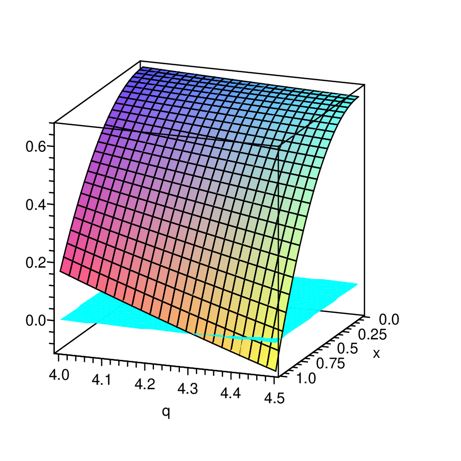
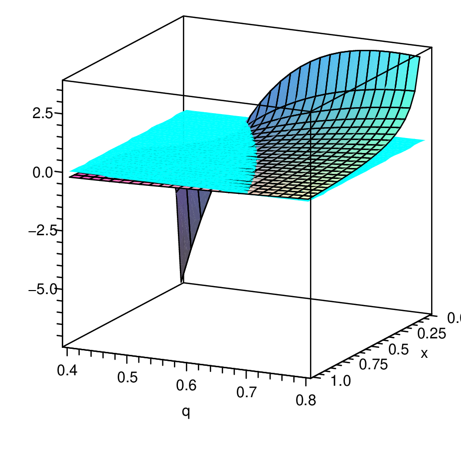
Due to the continuity of gq​(x)g_{q}(x) with respect to qq, we can always assure the convexity of gq​(x)g_{q}(x) for some region of qq slightly less than 1 or larger than 4. Furthermore, the continuity of l⁡(x,q)l(x,q) in Eq. (30) also assures the existence of q0q_{0} between 4 and 5, at which the convexity of gq​(x)g_{q}(x) starts being violated. However, it is generally hard to get an algebraic solution of such q0q_{0} since d2​gq​(x)d​x2\frac{{\rm d}^{2}g_{q}(x)}{{\rm d}x^{2}} in Eq. (25) is not an algebraic function with respect to qq. Here, we have a numerical way of calculation to test various values of xx and qq, and it is illustrated in Figure 1.

Refer to caption

(a)

Refer to caption

(b)

Fig. 1: The function values of d2​gq​(x)d​x2\frac{{\rm d}^{2}g_{q}(x)}{{\rm d}x^{2}} for 4≤q≤4.54\leq q\leq 4.5 and 0.4≤q≤0.80.4\leq q\leq 0.8 are illustrated in picture (a) and (b) respectively.

According to Figure 1, gq​(x)g_{q}(x) is convex for the region 0.7≤q≤4.20.7\leq q\leq 4.2, and thus the analytic formula of Tsallis-qq entanglement for two-qubit states in Eq. (23) can also be claimed for this region of qq.

III Multi-qubit Entanglement constraint in terms of Tsallis-qq Entanglement

Using concurrence as the bipartite entanglement measure, the monogamous property of a multi-qubit pure state |ψ⟩A1A2⋯An{\left|\psi\right\rangle}_{A_{1}A_{2}\cdots A_{n}} was shown to have a mathematical characterization as,

𝒞A1(A2⋯An)2≥𝒞A1​A22+⋯+𝒞A1​An2,\mathcal{C}_{A_{1}(A_{2}\cdots A_{n})}^{2}\geq\mathcal{C}_{A_{1}A_{2}}^{2}+\cdots+\mathcal{C}_{A_{1}A_{n}}^{2}, (32)

where 𝒞A1(A2⋯An)=𝒞(|ψ⟩A1(A2⋯An))\mathcal{C}_{A_{1}(A_{2}\cdots A_{n})}=\mathcal{C}({\left|\psi\right\rangle}_{A_{1}(A_{2}\cdots A_{n})}) is the concurrence of |ψ⟩A1A2⋯An{\left|\psi\right\rangle}_{A_{1}A_{2}\cdots A_{n}} with respect to the bipartite cut between A1A_{1} and the others, and 𝒞A1​Ai=𝒞⁡(ρA1​Ai)\mathcal{C}_{A_{1}A_{i}}=\mathcal{C}(\rho_{A_{1}A_{i}}) is the concurrence of the reduced density matrix ρA1​Ai\rho_{A_{1}A_{i}} for i=2,…,ni=2,\ldots,n [6, 7].

As a dual value to concurrence, Concurrence of Assistance (CoA) [16] of a bipartite state ρA​B\rho_{AB} is defined as

𝒞a(ρA​B)=max∑kpk𝒞(|ψk⟩A​B),\mathcal{C}^{a}(\rho_{AB})=\max\sum_{k}p_{k}\mathcal{C}({{\left|\psi_{k}\right\rangle}}_{AB}), (33)

where the maximum is taken over all possible pure state decompositions of ρA​B=∑kpk|ψk⟩A​B⟨ψk|\rho_{AB}=\sum_{k}p_{k}{\left|\psi_{k}\right\rangle}_{AB}{\left\langle\psi_{k}\right|}. Furthermore, it was also shown that there exists a polygamy (or dual monogamy) relation of multi-qubit entanglement in terms of CoA [17]: For any multi-qubit pure state |ψ⟩A1⋯An{\left|\psi\right\rangle}_{A_{1}\cdots A_{n}}, we have

𝒞A1(A2⋯An)2≤(𝒞A1​A2a)2+⋯+(𝒞A1​Ana)2,\mathcal{C}_{A_{1}(A_{2}\cdots A_{n})}^{2}\leq(\mathcal{C}^{a}_{A_{1}A_{2}})^{2}+\cdots+(\mathcal{C}^{a}_{A_{1}A_{n}})^{2}, (34)

where 𝒞A1​Aia\mathcal{C}^{a}_{A_{1}A_{i}} is the CoA of the reduced density matrix ρA1​Ai\rho_{A_{1}A_{i}} for i=2,…,ni=2,\ldots,n.

Here, we show that this monogamous and polygamous property of multi-qubit entanglement can also be characterized in terms of Tsallis-qq entanglement and TEoA. Before this, we provide an important property of the function gq​(x)g_{q}(x) in Eq. (20) for the proof of multi-qubit monogamy and polygamy relations.

For each q>0q>0, let us define a two-variable function mq​(x,y)m_{q}(x,y),

mq​(x,y):=gq​(x2+y2)−gq​(x)−gq​(y),m_{q}(x,y):=g_{q}\left(\sqrt{x^{2}+y^{2}}\right)-g_{q}(x)-g_{q}(y), (35)

on the domain 𝒟={(x,y)|0≤x,y,x2+y2≤1}{\mathcal{D}}=\{(x,y)|0\leq x,y,x^{2}+y^{2}\leq 1\}. Since mq​(x,y)m_{q}(x,y) is continuous on the domain 𝒟\mathcal{D} and analytic in the interior, its maximum or minimum values can arise only at the critical points or on the boundary of 𝒟\mathcal{D}. By taking the first-order partial derivatives of mq​(x,y)m_{q}(x,y), we have its gradient

∇mp​(x,y)=(∂mp​(x,y)∂x,∂mp​(x,y)∂y)\nabla m_{p}(x,y)=\left(\frac{\partial m_{p}(x,y)}{\partial x},\frac{\partial m_{p}(x,y)}{\partial y}\right) (36)

where

∂mq​(x,y)∂x=\displaystyle\frac{\partial m_{q}(x,y)}{\partial x}= α​x​[(1+1−x2−y2)q−1−(1+1−x2−y2)q−11−x2−y2−(1+1−x2)q−1−(1+1−x2)q−11−x2]\displaystyle\alpha x\left[\frac{{\left(1+\sqrt{1-x^{2}-y^{2}}\right)}^{q-1}-{\left(1+\sqrt{1-x^{2}-y^{2}}\right)}^{q-1}}{\sqrt{1-x^{2}-y^{2}}}-\frac{{\left(1+\sqrt{1-x^{2}}\right)}^{q-1}-{\left(1+\sqrt{1-x^{2}}\right)}^{q-1}}{\sqrt{1-x^{2}}}\right]
∂mq​(x,y)∂y=\displaystyle\frac{\partial m_{q}(x,y)}{\partial y}= α​y​[(1+1−x2−y2)q−1−(1+1−x2−y2)q−11−x2−y2−(1+1−y2)q−1−(1+1−y2)q−11−y2],\displaystyle\alpha y\left[\frac{{\left(1+\sqrt{1-x^{2}-y^{2}}\right)}^{q-1}-{\left(1+\sqrt{1-x^{2}-y^{2}}\right)}^{q-1}}{\sqrt{1-x^{2}-y^{2}}}-\frac{{\left(1+\sqrt{1-y^{2}}\right)}^{q-1}-{\left(1+\sqrt{1-y^{2}}\right)}^{q-1}}{\sqrt{1-y^{2}}}\right], (37)

with α=q2q​(q−1)\alpha=\frac{q}{2^{q}(q-1)}.

Suppose there exists (x0,y0)(x_{0},y_{0}) in the interior of 𝒟\mathcal{D} (that is, 0<x0,y0,x02+y02<10<x_{0},y_{0},x_{0}^{2}+y_{0}^{2}<1) such that ∇mp​(x0,y0)=0\nabla m_{p}(x_{0},y_{0})=0. From Eq. (37), it is straightforward to verify that ∇mp​(x0,y0)=0\nabla m_{p}(x_{0},y_{0})=0 is equivalent to

nq​(x0)=nq​(y0),n_{q}(x_{0})=n_{q}(y_{0}), (38)

for an analytic function

nq​(t)=(1+1−t2)q−1−(1+1−t2)q−11−t2,n_{q}(t)=\frac{{\left(1+\sqrt{1-t^{2}}\right)}^{q-1}-{\left(1+\sqrt{1-t^{2}}\right)}^{q-1}}{\sqrt{1-t^{2}}}, (39)

on 0<t<10<t<1. Furthermore, it is straightforward to see that d​nq​(t)d​t<0\frac{{\rm d}n_{q}(t)}{{\rm d}t}<0 for q>1q>1. In other words, nq​(t)n_{q}(t) is a strictly monotone-decreasing function with respect to tt for q>1q>1; therefore Eq. (38) implies x0=y0x_{0}=y_{0}. However, from Eq. (37), ∂mq​(x0,y0)∂x=0\frac{\partial m_{q}(x_{0},y_{0})}{\partial x}=0 together with x0=y0x_{0}=y_{0} imply that nq​(2​x0)=nq​(x0)n_{q}(\sqrt{2}x_{0})=n_{q}(x_{0}), which contradicts to the strict monotonicity of nq​(t)n_{q}(t). Thus mq​(x,y)m_{q}(x,y) has no vanishing gradient in the interior of 𝒟\mathcal{D}.

Now, let us consider the function values of mq​(x,y)m_{q}(x,y) on the boundary of 𝒟\mathcal{D}. If x=0x=0 or y=0y=0, it is clear that mq​(x,y)=0m_{q}(x,y)=0. For the case when x2+y2=1x^{2}+y^{2}=1, mq​(x,y)=0m_{q}(x,y)=0 becomes a single variable function

bq​(x)=\displaystyle b_{q}(x)= β⁡[(1+1−x2)q+(1−1−x2)q]\displaystyle\beta\left[\left(1+\sqrt{1-x^{2}}\right)^{q}+\left(1-\sqrt{1-x^{2}}\right)^{q}\right]
+β⁡[(1+x)q+(1−x)q−2−2q]\displaystyle+\beta\left[\left(1+x\right)^{q}+\left(1-x\right)^{q}-2-2^{q}\right] (40)

with β=1(q−1)​2q\beta=\frac{1}{(q-1)2^{q}}, which is an analytic function on 0≤x≤10\leq x\leq 1. For the case when q=2q=2 or 33, it is clear form Eq. (29) that mq​(x,y)=0m_{q}(x,y)=0, and thus bq​(x)=0b_{q}(x)=0. If qq is neither 2 nor 3, bq​(x)b_{q}(x) has only one critical point at x=12x=\frac{1}{\sqrt{2}} for any q>1q>1. Because bq​(0)=bq​(1)=0b_{q}(0)=b_{q}(1)=0, which are the function values at the boundary, the signs of the function values of bq​(x)b_{q}(x) are totally determined by that of bq​(12)b_{q}\left(\frac{1}{\sqrt{2}}\right), which is the function value at the critical point. Now, we have

bq​(12)=\displaystyle b_{q}\left(\frac{1}{\sqrt{2}}\right)= 2(q−1)​2q​[(1+12)q+(1−12)q]\displaystyle\frac{2}{(q-1)2^{q}}\left[\left(1+\frac{1}{\sqrt{2}}\right)^{q}+\left(1-\frac{1}{\sqrt{2}}\right)^{q}\right]
−1(q−1)​2q​(2+2q),\displaystyle-\frac{1}{(q-1)2^{q}}\left(2+2^{q}\right), (41)

whose function value with respect to qq is illustrated in Figure 2.

Refer to caption
Fig. 2: The function values of bq​(12)b_{q}\left(\frac{1}{\sqrt{2}}\right) with respect to qq for 1<q≤41<q\leq 4.

In other words, the function mq​(x,y)m_{q}(x,y) in Eq. (35) has no vanishing gradient in the domain 𝒟\mathcal{D} for q>1q>1, and its function values at the boundary of 𝒟\mathcal{D} is always nonpositive for 1≤q<21\leq q<2 and 3<q≤43<q\leq 4, whereas mq​(x,y)m_{q}(x,y) is always nonnegative for 2<q<32<q<3. Thus, we have

gq​(x2+y2)≤gq​(x)+gq​(y)g_{q}\left(\sqrt{x^{2}+y^{2}}\right)\leq g_{q}(x)+g_{q}(y) (42)

for 1<q<21<q<2 and 3<q<43<q<4, and

gq​(x2+y2)≥gq​(x)+gq​(y)g_{q}\left(\sqrt{x^{2}+y^{2}}\right)\geq g_{q}(x)+g_{q}(y) (43)

for 2<q<32<q<3. For the case when q=2q=2 or 3, we have

gq​(x2+y2)=gq​(x)+gq​(y).g_{q}\left(\sqrt{x^{2}+y^{2}}\right)=g_{q}(x)+g_{q}(y). (44)

Now, we are ready to have the following theorem, which is the monogamy inequality of multi-qubit entanglement in terms of Tsallis-qq entanglement.

Theorem 2.

For a multi-qubit state ρA1⋯An\rho_{A_{1}\cdots A_{n}} and 2≤q≤32\leq q\leq 3, we have

𝒯q(ρA1(A2⋯An))≥𝒯q(ρA1​A2)+⋯+𝒯q(ρA1​An){\mathcal{T}}_{q}\left(\rho_{A_{1}(A_{2}\cdots A_{n})}\right)\geq{\mathcal{T}}_{q}(\rho_{A_{1}A_{2}})+\cdots+{\mathcal{T}}_{q}(\rho_{A_{1}A_{n}}) (45)

where 𝒯q(ρA1(A2⋯An)){\mathcal{T}}_{q}\left(\rho_{A_{1}(A_{2}\cdots A_{n})}\right) is the Tsallis-qq entanglement of ρA1(A2⋯An)\rho_{A_{1}\left(A_{2}\cdots A_{n}\right)} with respect to the bipartite cut between A1A_{1} and A2⋯AnA_{2}\cdots A_{n}, and 𝒯q​(ρA1​Ai){\mathcal{T}}_{q}(\rho_{A_{1}A_{i}}) is the Tsallis-qq entanglement of the reduced density matrix ρA1​Ai\rho_{A_{1}A_{i}} for i=2,⋯,ni=2,\cdots,n.

Proof.

For the case when q=2q=2 or 33, Eq. (29) implies

𝒯2​(ρA​B)=𝒞A​B22,𝒯3​(ρA​B)=32​𝒞A​B2,{\mathcal{T}}_{2}\left(\rho_{AB}\right)=\frac{{{\mathcal{C}}_{AB}}^{2}}{2},~{\mathcal{T}}_{3}\left(\rho_{AB}\right)=\frac{3}{2}{{\mathcal{C}}_{AB}}^{2}, (46)

for any two-qubit mixed state or 2⊗d2\otimes d pure state ρA​B\rho_{AB} and its concurrence 𝒞A​B{\mathcal{C}}_{AB}. Thus, the monogamy inequality in Eq (45) follows from Eqs. (32) and (46).

For 2<q<32<q<3, We first prove the theorem for nn-qubit pure state |ψ⟩A1⋯An{\left|\psi\right\rangle}_{A_{1}\cdots A_{n}}. Note that Eq. (32) is equivalent to

𝒞A1(A2⋯An)≥𝒞A1​A22+⋯+𝒞A1​An2,\mathcal{C}_{A_{1}(A_{2}\cdots A_{n})}\geq\sqrt{\mathcal{C}_{A_{1}A_{2}}^{2}+\cdots+\mathcal{C}_{A_{1}A_{n}}^{2}}, (47)

for any nn-qubit pure state |ψ⟩A1(A2⋯An){\left|\psi\right\rangle}_{A_{1}(A_{2}\cdots A_{n})}. Thus, from Eq. (43) together with Eq. (47), we have

𝒯q(|ψ⟩A1(A2⋯An))=\displaystyle{\mathcal{T}}_{q}\left({\left|\psi\right\rangle}_{A_{1}(A_{2}\cdots A_{n})}\right)= gq(𝒞A1(A2⋯An))\displaystyle g_{q}\left(\mathcal{C}_{A_{1}(A_{2}\cdots A_{n})}\right)
≥\displaystyle\geq gq​(𝒞A1​A22+⋯+𝒞A1​An2)\displaystyle g_{q}\left(\sqrt{\mathcal{C}_{A_{1}A_{2}}^{2}+\cdots+\mathcal{C}_{A_{1}A_{n}}^{2}}\right)
≥\displaystyle\geq gq​(𝒞A1​A2)\displaystyle g_{q}\left(\mathcal{C}_{A_{1}A_{2}}\right)
+gq​(𝒞A1​A32+⋯+𝒞A1​An2)\displaystyle+g_{q}\left(\sqrt{\mathcal{C}_{A_{1}A_{3}}^{2}+\cdots+\mathcal{C}_{A_{1}A_{n}}^{2}}\right)
⋮\displaystyle~~~~~~~\vdots
≥\displaystyle\geq gq​(𝒞A1​A2)+⋯+gq​(𝒞A1​An)\displaystyle g_{q}\left(\mathcal{C}_{A_{1}A_{2}}\right)+\cdots+g_{q}\left(\mathcal{C}_{A_{1}A_{n}}\right)
=\displaystyle= 𝒯q​(ρA1​A2)+⋯+𝒯q​(ρA1​An)\displaystyle{\mathcal{T}}_{q}\left(\rho_{A_{1}A_{2}}\right)+\cdots+{\mathcal{T}}_{q}\left(\rho_{A_{1}A_{n}}\right) (48)

where the first equality is by the functional relation between the concurrence and the Tsallis-qq entanglement for 2⊗d2\otimes d pure states, the first inequality is by the monotonicity of gq​(x)g_{q}(x), the other inequalities are by iterative use of Eq. (43), and the last equality is by Theorem 1.

For a nn-qubit mixed state ρA1(A2⋯An)\rho_{A_{1}(A_{2}\cdots A_{n})}, let ρA1(A2⋯An)=∑jpj|ψj⟩A1(A2⋯An)⟨ψj|\rho_{A_{1}(A_{2}\cdots A_{n})}=\sum_{j}p_{j}{\left|\psi_{j}\right\rangle}_{A_{1}(A_{2}\cdots A_{n})}{\left\langle\psi_{j}\right|} be an optimal decomposition such that 𝒯q(ρA1(A2⋯An))=∑jpj𝒯q(|ψj⟩A1(A2⋯An)){\mathcal{T}}_{q}\left(\rho_{A_{1}(A_{2}\cdots A_{n})}\right)=\sum_{j}p_{j}{\mathcal{T}}_{q}\left({\left|\psi_{j}\right\rangle}_{A_{1}(A_{2}\cdots A_{n})}\right).

Because each |ψj⟩A1(A2⋯An){\left|\psi_{j}\right\rangle}_{A_{1}(A_{2}\cdots A_{n})} in the decomposition is an nn-qubit pure state, we have

𝒯q(ρA1(A2⋯An))=\displaystyle{\mathcal{T}}_{q}\left(\rho_{A_{1}(A_{2}\cdots A_{n})}\right)= ∑jpj𝒯q(|ψj⟩A1(A2⋯An))\displaystyle\sum_{j}p_{j}{\mathcal{T}}_{q}\left({\left|\psi_{j}\right\rangle}_{A_{1}(A_{2}\cdots A_{n})}\right)
≥\displaystyle\geq ∑jpj​(𝒯q​(ρA1​A2j)+⋯+𝒯q​(ρA1​Anj))\displaystyle\sum_{j}p_{j}\left({\mathcal{T}}_{q}\left(\rho^{j}_{A_{1}A_{2}}\right)+\cdots+{\mathcal{T}}_{q}\left(\rho^{j}_{A_{1}A_{n}}\right)\right)
=\displaystyle= ∑jpj​𝒯q​(ρA1​A2j)+⋯+∑jpj​𝒯q​(ρA1​Anj)\displaystyle\sum_{j}p_{j}{\mathcal{T}}_{q}\left(\rho^{j}_{A_{1}A_{2}}\right)+\cdots+\sum_{j}p_{j}{\mathcal{T}}_{q}\left(\rho^{j}_{A_{1}A_{n}}\right)
≥\displaystyle\geq 𝒯q​(ρA1​A2)+⋯+𝒯q​(ρA1​An),\displaystyle{\mathcal{T}}_{q}\left(\rho_{A_{1}A_{2}}\right)+\cdots+{\mathcal{T}}_{q}\left(\rho_{A_{1}A_{n}}\right), (49)

where ρA1​Aij\rho^{j}_{A_{1}A_{i}} is the reduced density matrix of |ψj⟩A1(A2⋯An){\left|\psi_{j}\right\rangle}_{A_{1}(A_{2}\cdots A_{n})} onto subsystem A1​AiA_{1}A_{i} for each i=2,⋯,ni=2,\cdots,n and the last inequality is by definition of Tsallis-qq entanglement for each ρA1​Ai\rho_{A_{1}A_{i}}. ∎

Now, let us consider the polygamy of multi-qubit entanglement using Tsallis-qq entropy. We first note that the function gq​(x)g_{q}(x) in Eq. (20) can also relate CoA and TEoA of a two-qubit state ρA​B\rho_{AB}: By letting ρA​B=∑ipi|ψi⟩A​B⟨ψi|\rho_{AB}=\sum_{i}p_{i}{\left|\psi_{i}\right\rangle}_{AB}{\left\langle\psi_{i}\right|} be an optimal decomposition for its CoA, that is,

𝒞a(ρA​B)=∑ipi𝒞(|ψi⟩A​B),\mathcal{C}^{a}\left(\rho_{AB}\right)=\sum_{i}p_{i}\mathcal{C}\left({\left|\psi_{i}\right\rangle}_{AB}\right), (50)

we have

gq​(𝒞a​(ρA​B))=\displaystyle g_{q}\left(\mathcal{C}^{a}\left(\rho_{AB}\right)\right)= gq(∑ipi𝒞(|ψi⟩A​B))\displaystyle g_{q}\left(\sum_{i}p_{i}\mathcal{C}\left({\left|\psi_{i}\right\rangle}_{AB}\right)\right)
≤\displaystyle\leq ∑ipigq(𝒞(|ψi⟩A​B))\displaystyle\sum_{i}p_{i}g_{q}\left(\mathcal{C}\left({\left|\psi_{i}\right\rangle}_{AB}\right)\right)
=\displaystyle= ∑ipi𝒯q(|ψi⟩A​B)\displaystyle\sum_{i}p_{i}{\mathcal{T}}_{q}\left({\left|\psi_{i}\right\rangle}_{AB}\right)
≤\displaystyle\leq 𝒯qa​(ρA​B)\displaystyle{\mathcal{T}}^{a}_{q}(\rho_{AB}) (51)

where the first inequality can be assured by the convexity of gq​(x)g_{q}(x) and the last inequality is by the definition of TEoA. Because gq​(x)g_{q}(x) is convex for 1≤q≤41\leq q\leq 4, Eq. (51) is thus true for this region of qq. Furthermore, gq​(x)g_{q}(x) satisfies the property of Eq. (42) for 1≤q≤21\leq q\leq 2 or 3≤q≤43\leq q\leq 4. Thus, we have the following theorem of the polygamy inequality in multi-qubit systems.

Theorem 3.

For any multi-qubit state ρA1⋯An\rho_{A_{1}\cdots A_{n}} and 1≤q≤21\leq q\leq 2 or 3≤q≤43\leq q\leq 4, we have

𝒯q(ρA1(A2⋯An))≤𝒯qa(ρA1​A2)+⋯+𝒯qa(ρA1​An){\mathcal{T}}_{q}\left(\rho_{A_{1}(A_{2}\cdots A_{n})}\right)\leq{\mathcal{T}}^{a}_{q}(\rho_{A_{1}A_{2}})+\cdots+{\mathcal{T}}^{a}_{q}(\rho_{A_{1}A_{n}}) (52)

where 𝒯q(ρA1(A2⋯An)){\mathcal{T}}_{q}\left(\rho_{A_{1}(A_{2}\cdots A_{n})}\right) is the Tsallis-qq entanglement of |ψ⟩A1(A2⋯An){\left|\psi\right\rangle}_{A_{1}\left(A_{2}\cdots A_{n}\right)} with respect to the bipartite cut between A1A_{1} and A2⋯AnA_{2}\cdots A_{n}, and 𝒯qa​(ρA1​Ai){\mathcal{T}}^{a}_{q}(\rho_{A_{1}A_{i}}) is the TEoA of the reduced density matrix ρA1​Ai\rho_{A_{1}A_{i}} for i=2,⋯,ni=2,\cdots,n.

Proof.

We first prove the theorem for a nn-qubit pure state, and generalize it into mixed states.

For the case when qq tends to 1, Tsallis-qq entanglement converges to EoA in Eq. (10). It was shown that the polygamy inequality of multi-qubit systems can be shown in terms of EoA [18]. For the case when q=2q=2 or 3, it is also straightforward from Eqs. (29) and (34).

For a nn-qubit pure state |ψ⟩A1(A2⋯An){\left|\psi\right\rangle}_{A_{1}(A_{2}\cdots A_{n})} and 1<q<21<q<2 or 3<q<43<q<4, let us first assume that (𝒞A1​A2a)2+⋯+(𝒞A1​Ana)2≤1(\mathcal{C}^{a}_{A_{1}A_{2}})^{2}+\cdots+(\mathcal{C}^{a}_{A_{1}A_{n}})^{2}\leq 1 in Eq. (34). Then we have

𝒯q(|ψ⟩A1(A2⋯An))\displaystyle{\mathcal{T}}_{q}\left({\left|\psi\right\rangle}_{A_{1}(A_{2}\cdots A_{n})}\right) =gq(𝒞A1(A2⋯An))\displaystyle=g_{q}({\mathcal{C}}_{A_{1}(A_{2}\cdots A_{n})})
≤gq​((𝒞A1​A2a)2+⋯+(𝒞A1​Ana)2)\displaystyle\leq g_{q}\left(\sqrt{(\mathcal{C}^{a}_{A_{1}A_{2}})^{2}+\cdots+(\mathcal{C}^{a}_{A_{1}A_{n}})^{2}}\right)
≤gq​(𝒞A1​A2a)\displaystyle\leq g_{q}\left(\mathcal{C}^{a}_{A_{1}A_{2}}\right)
+gq​((𝒞A1​A3a)2+⋯+(𝒞A1​Ana)2)\displaystyle~+g_{q}\left(\sqrt{(\mathcal{C}^{a}_{A_{1}A_{3}})^{2}+\cdots+(\mathcal{C}^{a}_{A_{1}A_{n}})^{2}}\right)
⋮\displaystyle~~~~~~~\vdots
≤gq​(𝒞A1​A2a)++⋯+gq​(𝒞A1​Ana)\displaystyle\leq g_{q}\left(\mathcal{C}^{a}_{A_{1}A_{2}}\right)++\cdots+g_{q}\left(\mathcal{C}^{a}_{A_{1}A_{n}}\right)
≤𝒯qa​(ρA1​A2)+⋯+𝒯qa​(ρA1​An),\displaystyle\leq{\mathcal{T}}^{a}_{q}\left(\rho_{A_{1}A_{2}}\right)+\cdots+{\mathcal{T}}^{a}_{q}\left(\rho_{A_{1}A_{n}}\right), (53)

where the first inequality is due to the monotonicity of the function gq​(x)g_{q}(x), the second and third inequalities are obtained by iterative use of Eq. (42), and the last inequality is by Eq. (51).

Now, let us assume that (𝒞A1​A2a)2+⋯+(𝒞A1​Ana)2>1(\mathcal{C}^{a}_{A_{1}A_{2}})^{2}+\cdots+(\mathcal{C}^{a}_{A_{1}A_{n}})^{2}>1. Due to the monotonicity of gq​(x)g_{q}(x), we first note that

𝒯q(|ψ⟩A1(A2⋯An))=\displaystyle{\mathcal{T}}_{q}\left({\left|\psi\right\rangle}_{A_{1}(A_{2}\cdots A_{n})}\right)= gq(𝒞(|ψ⟩A1(A2⋯An)))\displaystyle g_{q}\left({\mathcal{C}}\left({\left|\psi\right\rangle}_{A_{1}(A_{2}\cdots A_{n})}\right)\right)
≤\displaystyle\leq gq​(1)\displaystyle g_{q}\left(1\right)
=\displaystyle= 1q−1​(1−12q−1)\displaystyle\frac{1}{q-1}\left(1-\frac{1}{2^{q-1}}\right) (54)

for any multi-qubit pure state |ψ⟩A1(A2⋯An){\left|\psi\right\rangle}_{A_{1}(A_{2}\cdots A_{n})}, and q>1q>1. By letting γ=1q−1​(1−12q−1)\gamma=\frac{1}{q-1}\left(1-\frac{1}{2^{q-1}}\right), it is thus enough to show that 𝒯qa​(ρA1​A2)+⋯+𝒯qa​(ρA1​An)≥γ{\mathcal{T}}^{a}_{q}(\rho_{A_{1}A_{2}})+\cdots+{\mathcal{T}}^{a}_{q}(\rho_{A_{1}A_{n}})\geq\gamma.

Here, we note that there exists k∈{2,…,n−1}k\in\{2,\ldots,n-1\} such that

(𝒞A1​A2a)2+⋯+(𝒞A1​Aka)2≤1,\displaystyle(\mathcal{C}^{a}_{A_{1}A_{2}})^{2}+\cdots+(\mathcal{C}^{a}_{A_{1}A_{k}})^{2}\leq 1,
(𝒞A1​A2a)2+⋯+(𝒞A1​Ak+1a)2>1.\displaystyle(\mathcal{C}^{a}_{A_{1}A_{2}})^{2}+\cdots+(\mathcal{C}^{a}_{A_{1}A_{k+1}})^{2}>1. (55)

If we let

T:=(𝒞A1​A2a)2+⋯+(𝒞A1​Ak+1a)2−1,T:=(\mathcal{C}^{a}_{A_{1}A_{2}})^{2}+\cdots+(\mathcal{C}^{a}_{A_{1}A_{k+1}})^{2}-1, (56)

we have

γ=\displaystyle\gamma= gq​(1)\displaystyle g_{q}\left(1\right)
=\displaystyle= gq​((𝒞A1​A2a)2+⋯+(𝒞A1​Ak+1a)2−T)\displaystyle g_{q}\left(\sqrt{(\mathcal{C}^{a}_{A_{1}A_{2}})^{2}+\cdots+(\mathcal{C}^{a}_{A_{1}A_{k+1}})^{2}-T}\right)
≤\displaystyle\leq gq​((𝒞A1​A2a)2+⋯+(𝒞A1​Aka)2)\displaystyle g_{q}\left(\sqrt{(\mathcal{C}^{a}_{A_{1}A_{2}})^{2}+\cdots+(\mathcal{C}^{a}_{A_{1}A_{k}})^{2}}\right)
+gq​((𝒞A1​Ak+1a)2−T)\displaystyle~~~~~~+g_{q}\left(\sqrt{(\mathcal{C}^{a}_{A_{1}A_{k+1}})^{2}-T}\right)
≤\displaystyle\leq gq​(𝒞A1​A2a)+⋯+qq​(𝒞A1​Aka)+qq​(𝒞A1​Ak+1a)\displaystyle g_{q}\left(\mathcal{C}^{a}_{A_{1}A_{2}}\right)+\cdots+q_{q}\left(\mathcal{C}^{a}_{A_{1}A_{k}}\right)+q_{q}(\mathcal{C}^{a}_{A_{1}A_{k+1}})
≤\displaystyle\leq 𝒯qa​(ρA1​A2)+⋯+𝒯qa​(ρA1​An),\displaystyle{\mathcal{T}}^{a}_{q}(\rho_{A_{1}A_{2}})+\cdots+{\mathcal{T}}^{a}_{q}(\rho_{A_{1}A_{n}}), (57)

where the first inequality is by using Eq. (42) with respect to (𝒞A1​A2a)2+⋯+(𝒞A1​Aka)2(\mathcal{C}^{a}_{A_{1}A_{2}})^{2}+\cdots+(\mathcal{C}^{a}_{A_{1}A_{k}})^{2} and (𝒞A1​Ak+1a)2−T(\mathcal{C}^{a}_{A_{1}A_{k+1}})^{2}-T, the second inequality is by iterative use of Eq. (42) on (𝒞A1​A2a)2+⋯+(𝒞A1​Aka)2(\mathcal{C}^{a}_{A_{1}A_{2}})^{2}+\cdots+(\mathcal{C}^{a}_{A_{1}A_{k}})^{2}, and the last inequality is by Eq. (51).

For a nn-qubit mixed state ρA1(A2⋯An)\rho_{A_{1}(A_{2}\cdots A_{n})}, let ρA1(A2⋯An)=∑jpj|ψj⟩A1(A2⋯An)⟨ψj|\rho_{A_{1}(A_{2}\cdots A_{n})}=\sum_{j}p_{j}{\left|\psi_{j}\right\rangle}_{A_{1}(A_{2}\cdots A_{n})}{\left\langle\psi_{j}\right|} be an optimal decomposition for TEoA such that 𝒯qa(ρA1(A2⋯An))=∑jpj𝒯q(|ψj⟩A1(A2⋯An)){\mathcal{T}}^{a}_{q}\left(\rho_{A_{1}(A_{2}\cdots A_{n})}\right)=\sum_{j}p_{j}{\mathcal{T}}_{q}\left({\left|\psi_{j}\right\rangle}_{A_{1}(A_{2}\cdots A_{n})}\right). Because each |ψj⟩A1(A2⋯An){\left|\psi_{j}\right\rangle}_{A_{1}(A_{2}\cdots A_{n})} in the decomposition is an nn-qubit pure state, we have

𝒯qa(ρA1(A2⋯An))=\displaystyle{\mathcal{T}}^{a}_{q}\left(\rho_{A_{1}(A_{2}\cdots A_{n})}\right)= ∑jpj𝒯qa(|ψj⟩A1(A2⋯An))\displaystyle\sum_{j}p_{j}{\mathcal{T}}^{a}_{q}\left({\left|\psi_{j}\right\rangle}_{A_{1}(A_{2}\cdots A_{n})}\right)
≤\displaystyle\leq ∑jpj​(𝒯qa​(ρA1​A2j)+⋯+𝒯qa​(ρA1​Anj))\displaystyle\sum_{j}p_{j}\left({\mathcal{T}}^{a}_{q}\left(\rho^{j}_{A_{1}A_{2}}\right)+\cdots+{\mathcal{T}}^{a}_{q}\left(\rho^{j}_{A_{1}A_{n}}\right)\right)
=\displaystyle= ∑jpj​𝒯qa​(ρA1​A2j)+⋯+∑jpj​𝒯qa​(ρA1​Anj)\displaystyle\sum_{j}p_{j}{\mathcal{T}}^{a}_{q}\left(\rho^{j}_{A_{1}A_{2}}\right)+\cdots+\sum_{j}p_{j}{\mathcal{T}}^{a}_{q}\left(\rho^{j}_{A_{1}A_{n}}\right)
≤\displaystyle\leq 𝒯qa​(ρA1​A2)+⋯+𝒯qa​(ρA1​An),\displaystyle{\mathcal{T}}^{a}_{q}\left(\rho_{A_{1}A_{2}}\right)+\cdots+{\mathcal{T}}^{a}_{q}\left(\rho_{A_{1}A_{n}}\right), (58)

where ρA1​Aij\rho^{j}_{A_{1}A_{i}} is the reduced density matrix of |ψj⟩A1(A2⋯An){\left|\psi_{j}\right\rangle}_{A_{1}(A_{2}\cdots A_{n})} onto subsystem A1​AiA_{1}A_{i} for each i=2,⋯,ni=2,\cdots,n and the last inequality is by definition of TEoA for each ρA1​Ai\rho_{A_{1}A_{i}}. ∎

Although Theorem 3 provides the polygamy inequality of multi-qubit entanglement in terms of TEoA for 1≤q≤21\leq q\leq 2 or 3≤q≤43\leq q\leq 4, it is also clear that Eq. (52) is also true for qq slightly larger than 4 or less than 1 due to its continuity with respect to qq.

IV Conclusion

Using Tsallis-qq entropy, we have established a class of bipartite entanglement measures, Tsallis-qq entanglement, and provided its analytic formula in two-qubit systems for 1≤q≤41\leq q\leq 4. Based on the functional relation between concurrence and Tsallis-qq entanglement, we have shown that the monogamy of multi-qubit entanglement can be mathematically characterized in terms of Tsallis-qq entanglement for 2≤q≤32\leq q\leq 3. We have also provided a polygamy inequality of multi-qubit entanglement in terms of TEoA for 1≤q≤21\leq q\leq 2 and 3≤q≤43\leq q\leq 4.

The class of monogamy and polygamy inequalities of multi-qubit entanglement we provided here consists of infinitely many inequalities parameterized by qq. We believe that our result will provide useful tools and strong candidates for general monogamy and polygamy relations of entanglement in multipartite higher-dimensional quantum systems, which is one of the most important and necessary topics in the study of multipartite quantum entanglement.

Acknowledgments

This work was supported by iCORE, MITACS and USARO.

References

  • [1] C. H. Bennett, G. Brassard, C. Crepeau, R. Jozsa, A. Peres and W. K. Wootters, Phys. Rev. Lett. 70, 1895 (1993).
  • [2] W. K. Wootters and W. H. Zurek, Nature 299, 802 (1982).
  • [3] B. M. Terhal, IBM J. Research and Development 48, 71 (2004).
  • [4] L. Masanes, Phys. Rev. Lett. 102, 140501 (2009).
  • [5] W. K. Wootters, Phys. Rev. Lett. 80, 2245 (1998).
  • [6] V. Coffman, J. Kundu and W. K. Wootters, Phys. Rev. A 61, 052306 (2000).
  • [7] T. Osborne and F. Verstraete, Phys. Rev. Lett. 96, 220503 (2006).
  • [8] C. H. Bennett, D. P. DiVincenzo, J. A. Smolin and W. K. Wootters, Phys. Rev. A 54, 3824 (1996).
  • [9] A. Rényi, Proceedings of the Fourth Berkeley Symposium on Mathematics, Statistics and Probability (University of California Press, Berkeley, 1960) 1, p. 547-561 .
  • [10] R. Horodecki, P. Horodecki and M. Horodecki, Phys. Lett. A 210, 377 (1996).
  • [11] C. Tsallis, J. Stat. Phys. 52, 479 (1988).
  • [12] P. T. Landsberg and V. Vedral, Phys. Lett. A 247, 211 (1998).
  • [13] J. S. Kim and B. C. Sanders, arXiv.org:0911.5180 (2009).
  • [14] O. Cohen, Phys. Rev. Lett. 80, 2493 (1998).
  • [15] Due to the existence of the decomposition satisfying Eqs (21) and (22), we have
    gq​(𝒞⁡(ρA​B))=\displaystyle g_{q}\left(\mathcal{C}(\rho_{AB})\right)= gq(∑ipi𝒞(|ϕi⟩A​B))\displaystyle g_{q}\left(\sum_{i}p_{i}\mathcal{C}({\left|\phi_{i}\right\rangle}_{AB})\right)
    =\displaystyle= ∑ipigq(𝒞(|ϕi⟩A​B))\displaystyle\sum_{i}p_{i}g_{q}\left(\mathcal{C}({\left|\phi_{i}\right\rangle}_{AB})\right)
    =\displaystyle= ∑ipi𝒯q(|ϕi⟩A​B)\displaystyle\sum_{i}p_{i}{\mathcal{T}}_{q}({\left|\phi_{i}\right\rangle}_{AB})
    ≥\displaystyle\geq 𝒯q​(ρA​B).\displaystyle{\mathcal{T}}_{q}\left(\rho_{AB}\right).
    Conversely, the existence of the optimal decomposition of ρA​B=∑jqj|μj⟩A​B⟨μj|\rho_{AB}=\sum_{j}q_{j}{\left|\mu_{j}\right\rangle}_{AB}{\left\langle\mu_{j}\right|} for Tsallis-qq entanglement leads us to
    𝒯q​(ρA​B)=\displaystyle{\mathcal{T}}_{q}\left(\rho_{AB}\right)= ∑jqj𝒯q(|μj⟩A​B)\displaystyle\sum_{j}q_{j}{\mathcal{T}}_{q}\left({\left|\mu_{j}\right\rangle}_{AB}\right)
    =\displaystyle= ∑jqjgq(𝒞(|μj⟩A​B))\displaystyle\sum_{j}q_{j}g_{q}\left({\mathcal{C}}({\left|\mu_{j}\right\rangle}_{AB})\right)
    ≥\displaystyle\geq gq(∑jqj𝒞(|μj⟩A​B))\displaystyle g_{q}\left(\sum_{j}q_{j}{\mathcal{C}}({\left|\mu_{j}\right\rangle}_{AB})\right)
    ≥\displaystyle\geq gq​(𝒞⁡(ρA​B)),\displaystyle g_{q}\left({\mathcal{C}}(\rho_{AB})\right),
    where the first and second inequalities are due to the convexity and monotonicity of gq​(x)g_{q}(x).
  • [16] T. Laustsen, F. Verstraete and S. J. van Enk, Quantum Inf. Comput. 3, 64 (2003).
  • [17] G. Gour, S. Bandyopadhay and B. C. Sanders, J. Math. Phys. 48, 012108 (2007).
  • [18] F. Buscemi, G. Gour and J. S. Kim, Phys. Rev. A 80, 012324 (2009).