Heegaard structure respects complicated JSJ decompositions
Abstract.
Let be a 3-manifold with torus boundary components and . Let be a homeomorphism, the manifold obtained from by gluing to via the map , and the image of in . We show that if is “sufficiently complicated” then any incompressible or strongly irreducible surface in can be isotoped to be disjoint from . It follows that every Heegaard splitting of a 3-manifold admitting a “sufficiently complicated” JSJ decomposition is an amalgamation of Heegaard splittings of the components of the JSJ decomposition.
1. Introduction
Let be a (possibly disconnected) 3-manifold with homeomorphic boundary components and . Let be a homeomorphism, and let be the manifold obtained from by gluing to via the map . Finally, let denote the image of in . So-called incompressible and strongly irreducible surfaces have been seen to be vital to the study of 3-manifolds. A natural question is how such surfaces in are related to surfaces in . In many cases it is known that with some assumption on the map , a class of such surfaces in can be isotoped to be disjoint from . In other words, each surface in the class is isotopic into the original manifold . When this conclusion follows, then we say is a barrier for the class.
If is separating and its genus is greater than one, then Lackenby [Lac04] and Souto [Sou] have independently shown that if is “sufficiently complicated” (in different contexts), then is a barrier for all incompressible and strongly irreducible surfaces of bounded genus. Li [Li07] also obtained a similar result, including the case that is a (possibly non-separating) torus. In some cases it is even known that is a barrier for all incompressible and strongly irreducible surfaces regardless of their genus. For example, this follows from [BSS06] when is a separating torus in .
In this paper we look at the situation when the gluing surface is a torus in that may be non-separating. Our main result is that the same conclusion holds: when is “sufficiently complicated” the surface is a barrier for all incompressible and strongly irreducible surfaces, regardless of their genus. A consequence of this is that all Heegaard splittings of arise from Heegaard splittings of in a natural way.
To prove our main result, the first challenge is to construct a reasonable definition of the term “sufficiently complicated” that depends only on the manifold . This is accomplished in Section 2, where we construct a complexity for gluing maps between two torus boundary components of a 3-manifold called the -distance, where depends on the class of surfaces under consideration. We then establish our first theorem:
Theorem 1.1.
Let be a compact, orientable, irreducible 3-manifold with incompressible boundary and let and be two torus components of . Let be a gluing map whose 1-distance is at least two. Then every closed, orientable, incompressible and strongly irreducible surface in can be isotoped to be disjoint from the image of in .
That is, a sufficiently complicated gluing map between torus boundary components of a 3-manifold creates a barrier to all incompressible and strongly irreducible surfaces. The most interesting case of Theorem 1.1 is when is connected, since similar results were previously obtained in [BSS06] for the case that is disconnected. In the special case when this follows from [CS99].
The proof of Theorem 1.1 is given in Section 3, considering the incompressible and strongly irreducible cases separately. In Section 4 we review the definitions of generalized Heegaard splitting and amalgation, and then extend the definition of -distance to gluings along arbitrarily many tori. This allows us to put everything together to prove the following theorem about Heegaard splittings of certain 3-manifolds with non-trivial JSJ decompositions (see Section 4 for relevant definitions):
Theorem 1.2.
Let be a closed, irreducible, orientable 3-manifold that admits a JSJ decomposition whose collection of JSJ tori has -distance at least 2. Then every Heegaard splitting of is an amalgamation of Heegaard splittings of the components of the JSJ decomposition of over the gluing maps.
Theorem 1.2 greatly simplifies the Heegaard structure of 3-manifolds that are “sufficiently complicated” in the above sense. For example, despite being toroidal, such manifolds admit only finitely many Heegaard splittings of any given genus up to isotopy (see Corollary 4.13).
In the proof of Theorem 1.1 we show that need only to have -distance one to create a barrier to incompressible surfaces. In Section 5 we address the question of the existence of -distance one gluing maps. There we show the following:
Theorem 1.3.
Let be a compact, orientable, irreducible 3-manifold with incompressible boundary and let and be two torus components of . Let and be homeomorphisms, where is Anosov. Then for each there exists a positive integer such that for , the map has -distance at least one.
As above, the most interesting case is when is connected since otherwise this result is implied by [Hat82]. Theorems 1.1 and 1.3 imply that the composition of any gluing map between two torus boundary components of some 3-manifold with a sufficiently high power of an Anosov map creates a barrier to all incompressible surfaces. We expect a similar result holds for strongly irreducible surfaces as well.
2. Boundary slopes of surfaces that meet the 2-skeleton normally
Let be a compact, orientable, irreducible, triangulated 3-manifold consisting of one or two components11 1 The results for this section in the case that has two components have been obtained previously in [Hat82] and [JS03]. While our focus is therefore on the case that is connected, the results we establish here are general and include these previously obtained results in our own terminology, which we provide for completeness and ease of exposition in later sections.. Presently we shall define what it means for a surface to meet the 2-skeleton of the triangulation normally. Such surfaces can then be broken up into compatibility classes with certain properties (see Definitions 2.5 and 2.7). Suppose and are torus components of . The main result of this section is an extension of Hatcher’s theorem [Hat82], [FO84] from slopes of essential surfaces to slopes of surfaces which meet the 2-skeleton of a triangulation normally. Namely, we show that each compatibility class determines an element of such that for each , , where is the slope of . These maps will allow us to define the complexity for gluing maps referred to in Section 1.
Much of the terminology for this section is based on that of Jaco and Sedgwick [JS03]. Also, the reader is referred to [JT95] for a more elementary introduction to normal surface theory.
Fix a triangulation of that restricts to one-vertex triangulations on and . Such triangulations exist by [JS03].
Definition 2.1.
A properly embedded arc in a 2-simplex of is normal if it connects distinct 1-simplices. A loop on the boundary of a tetrahedron is normal if it consists of normal arcs. A normal isotopy of such a loop is an isotopy that restricts to an isotopy in each boundary simplex of the tetrahedron. It is well known that each normal loop consists of 3 or normal arcs. The complexity of a normal loop which consists of 3 arcs is zero, and of a normal loop that consists of arcs is .
Definition 2.2.
A surface in is normal with respect to the 2-skeleton if it meets the boundary of every tetrahedron in a collection of normal loops. The complexity of such a surface is the maximum complexity of all such normal loops.
Examples 2.3.
- (1)
Haken [Hak68] showed that surfaces that are both incompressible and -incompressible can be isotoped to be normal; i.e., to be complexity 0 surfaces, and in addition to meet each tetrahedron in disks.
- (2)
It follows from work of Rubinstein [Rub95] and Stocking [Sto00] that Heegaard surfaces may be isotoped to be complexity at most 1, provided they are strongly irreducible. This condition means that any compressing disk on one side of such a Heegaard surface meets every compressing disk on the other, and that there is at least one such disk on each side.
- (3)
It follows from [BDTS] that strongly irreducible surfaces that are also -strongly irreducible can be isotoped to be complexity 1. Such surfaces have the additional property that any compressing or -compressing disk on one side meets every compressing and -compressing disk on the other.
Definition 2.4.
Two surfaces and that are normal with respect to the 2-skeleton are compatible if on the boundary of each tetrahedron , the normal loops and can be normally isotoped to be disjoint.
It is well known that if and are compatible, and and are components of and , respectively, of length larger than 3, then and are normally isotopic.
Definition 2.5.
A maximal (with respect to inclusion) set of surfaces that are normal with respect to the 2-skeleton and pairwise compatible forms a compatibility class.
A choice of a normal loop of length larger than 3 on the boundary of each tetrahedron thus determines at most one compatibility class.
Definition 2.6.
The complexity of a non-empty compatibility class is the maximum of the complexities of the surfaces contained in the class.
 |
Following [JS03], a (not necessarily connected) normal curve in a one-vertex triangulation of a torus is parameterized by a free choice of normal coordinates in exactly one of the two triangles, forcing the normal coordinates in the other triangle to be equal, (see Figure 1). Projectively, this set corresponds to the points with rational coordinates in the 2-simplex pictured in Figure 2.
 |
A normal curve has type if . Of course, a normal curve with a non-unique minimal coordinate has more than one type, and will be all three types precisely when it consists entirely of trivial curves.
Definition 2.7.
The type of a surface in is the pair of types of the boundary curves of on and , respectively. A typed compatibility class is a compatibility class restricted to surfaces of the same type.
Remark 2.8.
Since there are a bounded number of distinct normal isotopy classes of loops of bounded complexity on the boundary of a single tetrahedron, then it follows that there are a bounded number of typed compatibility classes with complexity less than a specified bound. For instance, there are at most typed compatibility classes of complexity zero surfaces, each determined by a pair of boundary types and a choice of a length 4 loop in each of the tetrahedra.
Let and be normal arcs in an oriented triangle . Then and can be isotoped, keeping their boundaries fixed, so that they intersect in at most one point. We define the normal sign of the point , if it exists, as follows. There is at least one arc of the 1-skeleton of that connects to . Then we say is
- •
positive if the orientation on induced by the orientation of points from to , and
- •
negative otherwise (see Figure 3).
 |
Lemma 3.5 of [JS03] shows that normal isotopy and isotopy are equivalent for normal curves in a one-vertex triangulation of a torus. Moreover,
Lemma 2.9.
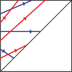
Suppose that normal curves of the same type, and , have been normally isotoped to intersect minimally in a one-vertex triangulation of a torus. Then all intersection points between and have the same normal sign.
Proof.
Without loss of generality assume that and are both of type 3. Since they intersect minimally, each trivial component of and is disjoint from every other component. Let and be obtained by removing trivial components from and respectively. Then and do not possess normal arcs of the third type and can be consistently oriented by applying orientations to the remaining two arc types as in Figure 4.
 |
Now consider an intersection between a normal arc of and a normal arc of . Since the curves are of type 3, the algebraic sign is equal to the normal sign of the intersection point (see Figure 5). We have already observed, however, that and intersect minimally, hence all intersections have the same algebraic sign. It follows that all intersection points have positive normal sign or all have negative normal sign.
 |
∎
Lemma 2.10.
Let and be surfaces meeting the 2-skeleton of normally, in the same typed compatibility class, whose intersection with is contained in . Suppose and are normally isotoped to intersect minimally. Let and designate their normal boundary curves, oriented by type (see Figure 4). Then the algebraic intersection numbers are related by .
Proof.
Consider a tetrahedron, . Let denote a component of , and a component of . Since and intersect minimally, we may assume each normal arc of and is a straight line segment.
As and are compatible, there is an isotopy from to a normal loop in that is disjoint from . We can choose such an isotopy that interpolates the intersections with the 1-skeleton and so that for all , each normal arc of is a straight line segment. Furthermore, by adjusting the rate of interpolation, we may assume that the isotopy is in general position. Let denote the critical values of , i.e. the values of such that and do not intersect transversely on . It follows that for each , includes a point of the 1-skeleton. Let denote the difference between the number of positive and negative intersection points of and , when their intersection is in general position.
 |
Just before (or after) , meets as in Figure 6. Here we see two intersections, one of each normal sign, of which cancel as increases through . It follows that . As , we conclude is zero for all non-critical . It follows that there are an equal number of positive and negative normal signs on the intersections of and on .
Note that the induced orientations on an interior face are opposite from the two (not necessarily distinct) tetrahedra on either side of it. Therefore the normal sign of each intersection point is opposite with respect to each orientation. It follows that the sum of the normal intersections is zero when summed over only faces in the boundary. By Lemma 2.9, on each boundary component , each intersection point between and has the same sign. Therefore the positive and negative intersections between and on happen on different tori. Since they agree with the algebraic intersection numbers there, . ∎
The above result is particularly relevant to the case that is connected. In the case that consists of two components (each having a torus boundary component), Lemma 2.10 implies that every surface in a given compatibility class (intersecting in only) intersects each boundary torus in a unique slope.
Fix homology bases for and so that the orientation on agrees with the induced boundary orientation, and the orientation on disagrees with the induced boundary orientation. A slope is the isotopy class of a closed and connected essential curve in a torus. With our choice of basis for the homology of the torus, slopes are parameterized by . If is an embedded but disconnected curve that contains an essential curve, then we will define the slope of , denoted , to be the isotopy class of one of its essential connected components. The slope of a surface on a torus is the slope of an essential component of its intersection with . An element acts on the set of slopes as a linear fractional transformation, i.e., .
Lemma 2.11.
Let be a typed compatibility class of surfaces that meet the 2-skeleton normally. Then there exists an element such that for all where , , and , the element maps the slope of on to the slope of on , i.e. .
Proof.
There are two cases. In the first case, we assume that all surfaces meet in a single slope . Since any pair of these surfaces can be isotoped to be disjoint on , it follows from Lemma 2.10 that they can also be isotoped to be disjoint on . Hence all surfaces have the same slope on . With respect to the given bases on choose a particular element so that .
In the second case, we suppose that there are two surfaces and in which meet in distinct slopes, and hence in distinct slopes on . Let and be column vectors expressing the homology classes and , respectively. Construct the matrices . By Lemma 2.10 and because one of the chosen homology bases disagrees with the induced boundary orientations, . Now let . Note that has determinant 1, and thus can be regarded as an element of . Restricting the equation to each column vector of , we obtain and , i.e., is a map between the homology classes of the boundaries of these surfaces.
We need to show this holds for any other surface . Suppose that meets the boundary with homology classes and . Since and are independent, any other vector is uniquely determined by its intersections with them. We check that and have the same number of intersections with :
by Lemma 2.10. The calculation for is identical and thus maps to , as desired.
Finally, in this second case, we regard as a linear fractional transformation so that it acts on slopes rather than homology classes. ∎
We now define the notion of distance of a map that glues together two torus boundary components of a 3-manifold. To do this, we first define the Farey graph:
Definition 2.12.
Let be a torus. The Farey graph for is the graph formed by taking a vertex for each slope on , and connecting two vertices with an edge if simple closed curve representatives of the two corresponding slopes can be isotoped to intersect in one point on . The distance between two slopes is taken to be the minimum length of a path in the Farey graph between the corresponding vertices.
Definition 2.13.
Fix a number . For each typed compatibility class of surfaces of complexity at most (of which there are a finite number by Remark 2.8), let be the element of given by Lemma 2.11. Suppose is a gluing map. Then we say has distance if the minimum distance (in the Farey graph of ), over all slopes on , of and the slope of , is . The -distance of the gluing map is then the minimum, over all maps , of the distances of .
Note that if the -distance of is non-zero then each composition fixes no slope. Also, observe that if , then the -distance of is greater than or equal to the -distance of .
3. Proof of Theorem 1.1.
In this section we present the proof of Theorem 1.1. This is broken up into two cases, depending on whether the surfaces we are concerned with are incompressible or strongly irreducible.
3.1. The incompressible case.
Lemma 3.1.
Let be a compact, irreducible, orientable 3-manifold with incompressible, if non-empty. Suppose and are closed, essential surfaces in . Then may be isotoped to be transverse to with every component of incompressible in the respective submanifold of .
Proof.
Isotope so that it meets transversally, and so that is minimal. Let be a loop of . Let be a compressing disk for . As is incompressible in , bounds a subdisk of , where necessarily . As is incompressible, every loop of must be inessential on . We conclude contains some loop that is inessential on both surfaces. But then by a standard innermost disk argument we can lower , a contradiction. Thus, must be incompressible in .
We must now establish that each component of is incompressible. Choose the compressing disk for a component of whose interior meets the other components in a minimal number of loops. Let be such a loop that is innermost on . Then bounds a subdisk of , and . As is incompressible, is inessential on . But then by a similar innermost disk argument we may reduce the number of intersections of with , a contradiction. ∎
Lemma 3.2.
Let be a compact, orientable, irreducible 3-manifold. Let be an orientable, connected, properly embedded, incompressible surface in , such that each loop of is contained in a torus component of . Then either is a boundary-parallel annulus or is -incompressible.
Proof.
Suppose there is a -compression for . Let be the component of that meets . Then is an arc, . There are now two cases. Suppose first connects two distinct loops of . As is a torus, these loops cobound an annulus of . Let denote the disk obtained from by removing a neighborhood of . Then two parallel copies of , together with the disk , is a disk whose boundary is on . As is incompressible, we conclude is a boundary-parallel annulus.
The second case is when connects some loop of to itself. Then , together with an arc of , cobounds a subdisk of . The disk is then a compressing disk for , a contradiction. ∎
We now establish the incompressible case of Theorem 1.1. Recall that is assumed to be a 3-manifold with incompressible boundary, is a gluing map between two torus components of , and is the resulting 3-manifold. Let be the image of in . Fix a triangulation of as in Section 2. Let be a closed, orientable, incompressible surface in .
By Lemma 3.1 we can isotope so that is incompressible in . If, for some , every component of that meets can be isotoped into a neighborhood of , then we can isotope in to miss entirely, and the result follows. Otherwise, by Lemma 3.2, for each there is a component of that meets and is both incompressible and -incompressible. Let then be a (possibly disconnected) subsurface of , which is properly embedded in , is incompressible, -incompressible, and meets both and .
By [Hak68] can be isotoped to be a normal surface with respect to . In this position, is a complexity zero surface in such that .
3.2. The strongly irreducible case.
When the surface is strongly irreducible, we may appeal to the results of [BSS06]. Lemmas 3.3 and 3.5 below, taken from that paper, will play the roles that Lemmas 3.1 and 3.2 played in the previous subsection.
Lemma 3.3.
[BSS06] Let be a compact, irreducible, orientable 3-manifold with incompressible, if non-empty. Suppose , where is a strongly irreducible Heegaard surface. Suppose further that contains an incompressible, orientable, closed, non-boundary parallel surface . Then either
- •
may be isotoped to be transverse to , with every component of incompressible in the respective submanifold of , or
- •
may be isotoped to be transverse to , with every component of incompressible in the respective submanifold of except for exactly one strongly irreducible component, or
- •
may be isotoped to meet in a single saddle tangency (and transverse elsewhere), with every component of incompressible in the respective submanifold of .
When is a torus we can rule out the third conclusion of this lemma, and thereby obtain the following corollary:
Corollary 3.4.
Let be a compact, irreducible, orientable 3-manifold with incompressible, if non-empty. Suppose , where is a strongly irreducible Heegaard surface. Suppose further that contains an essential torus . Then may be isotoped to be transverse to with every component of incompressible in the respective submanifold of except for at most one strongly irreducible component.
Proof.
Suppose has been isotoped to meet in a single saddle tangency (and transverse elsewhere), with every component of incompressible in the respective submanifold of . Then must be essential on and both copies of on . This implies that isotoping by pushing the saddle tangency slightly past in either direction yields essential curves of intersection on . This is impossible, however, as is a torus, and resolving a saddle tangency in this way must produce an inessential curve on one side or the other. ∎
Lemma 3.5.
[BSS06] Let be a knot manifold. Let be a separating, properly embedded, connected surface in which is strongly irreducible, has non-empty boundary, and is not peripheral. Then either is -strongly irreducible or is at most distance one from the boundary of some properly embedded surface which is both incompressible and -incompressible.
In [BSS06] the term knot manifold was used to refer to a 3-manifold with a single boundary component, which is homeomorphic to a torus. However, the proof of Lemma 3.5 given in [BSS06] only uses the fact that each boundary component of the surface is contained in a torus component of .
We now proceed with the proof of the strongly irreducible case of Theorem 1.1. As before, is a 3-manifold with incompressible boundary, is a gluing map between two torus components of , is the resulting 3-manifold, and is the image of in . Fix a triangulation of as in Section 2. Let be a closed, strongly irreducible surface in .
By Corollary 3.4 we can isotope so that every component of is incompressible in , with the exception of at most one strongly irreducible component. If, for some , every component of that meets can be isotoped into a neighborhood of , then we can isotope in to miss entirely, and the result follows. Otherwise, either by Lemma 3.2 or by Lemma 3.5 there is a (possibly disconnected) surface , which is properly embedded in , is either incompressible and -incompressible or strongly irreducible and -strongly irreducible, and meets both and . Furthermore, the slope of is at most distance one from the slope of in the Farey graph of .
By [Hak68] and [BDTS] the surface can be isotoped to be a complexity zero or one surface in . Let denote the typed compatibility class of . Then by Lemma 2.11, . It follows that translates the slope of at most distance one in the Farey graph of , and thus the map has 1-distance zero or one. This concludes the proof of Theorem 1.1.
4. Heegaard splittings of 3-manifolds with sufficiently complicated JSJ decompositions are amalgamations.
Generalized Heegaard splittings were first introduced by Scharlemann and Thompson in [ST94]. Here we review some of the basic definitions of this theory (articulated with the language and notation given in [Bac08]) and provide an application of Theorem 1.1.
Definition 4.1.
A compression body is a 3-manifold which can be obtained by starting with some closed, orientable, connected surface, , forming the product , attaching some number of 2-handles to , and capping off all resulting 2-sphere boundary components that are not contained in with 3-balls. The boundary component is referred to as . The rest of the boundary is referred to as .
Definition 4.2.
A Heegaard splitting of a 3-manifold is an expression of as a union , where and are compression bodies that intersect in a transversally oriented surface . If is a Heegaard splitting of then we say is a Heegaard surface.
Definition 4.3.
A complex is the spine of a Heegaard splitting of if
- (1)
is the union of some subset of and a properly embedded graph in .
- (2)
is parallel to the frontier of a neighborhood of in .
Definition 4.4.
A generalized Heegaard splitting (GHS) of a 3-manifold is a pair of sets of pairwise disjoint, transversally oriented, connected surfaces, and (called the thick levels and thin levels, respectively), which satisfies the following conditions.
- (1)
Each component of meets a unique element of , and is a Heegaard surface in . Henceforth we will denote the closure of the component of that contains an element as .
- (2)
As each Heegaard surface is transversally oriented, we can consistently talk about the points of that are “above” or “below” . Suppose . Let and be the submanifolds on each side of . Then is below if and only if it is above .
- (3)
There is a partial ordering on the elements of which satisfies the following: Suppose is an element of , is a component of above , and is a component of below . Then .
Definition 4.5.
A GHS of is strongly irreducible if every element is strongly irreducible in .
Theorem 4.6.
[ST94] The thin levels of a strongly irreducible GHS are incompressible.
Corollary 4.7.
Let be a 3-manifold with incompressible boundary and let and be two torus components of . Let be a gluing map whose 1-distance is at least two, and let be the image of in . Then is isotopic to a thin level of every strongly irreducible GHS of .
Proof.
Let be a strongly irreducible GHS of . By Theorem 4.6, the thin levels of are incompressible. By Theorem 1.1, such surfaces can be isotoped to be disjoint from . But then lies in , for some thick level . As is strongly irreducible we may again apply Theorem 1.1 to conclude can be isotoped be disjoint from in . But then lies in a compression body. The only incompressible surfaces in a compression body are isotopic to negative boundary components, and all such components are thin levels of . ∎
The GHS determines a unique Heegaard splitting of , called its amalgamation, a generalization of a procedure with the same name given in [Sch93]. The definition provided here follows the version given in [Bac08], and is illustrated schematically in Figure 7. The dark lines in the figure represent a complex which is the spine of a Heegaard splitting of the manifold pictured. This complex has three parts. The first are those subsurfaces of that lie below thick levels. The second part is a collection of loops that lies entirely in compression bodies below thick levels. Finally, the third part is a collection of vertical arcs that connect the other two parts through compression bodies that lie above thick levels.
 |
The following result about amalgamation is implicit in [ST94]:
Lemma 4.8.
Suppose is a compact, orientable 3-manifold with incompressible boundary. Then every Heegaard splitting of is the amalgamation of some strongly irreducible GHS.
Definition 4.9.
Suppose is a collection of 3-manifolds, and is obtained from this collection by gluing pairs of boundary components by a collection of maps . Let be a GHS of whose thin levels are precisely the images of the boundary components of in . Then the thick levels of are a set , where is a Heegaard surface in . The amalgamation of is then said to be the amalgamation of the Heegaard surfaces over the maps .
Now we extend the notion of -distance to gluings along multiple tori.
Definition 4.10.
Let denote a collection of pairwise disjoint, pairwise non-parallel, essential tori in a compact, orientable 3-manifold . Let be an ordering of the elements of . Let denote the manifold obtained from by cutting along all tori in . Let and denote the copies of on . Let denote the manifold obtained from by the gluing , defined so that the manifold . Then we say the ordered collection has -distance if there is a triangulation of each manifold so that the minimum of the -distances of the maps is precisely . The -distance of is the maximum -distance taken over all of its orderings .
The following is a celebrated theorem of 3-manifold topology.
Theorem 4.11.
Definition 4.12.
The decomposition of given in Theorem 4.11 is called the JSJ decomposition of , and is called the collection of JSJ tori in .
We are now ready to prove Theorem 1.2.
Proof.
Let be a Heegaard surface of , and let denote the collection of JSJ tori in . Let be an ordering of the JSJ tori realizing the 1-distance of , and let be the corresponding submanifolds as given in Definition 4.10. Now for some , is an amalgamation of splittings of the components of the manifold , where at worst . Let be the smallest value of such that arises from an amalgamation of splittings of the components of over the maps . We claim , and thus the result follows.
Let denote the (possibly disconnected) Heegaard surface of whose amalgamation over the maps is . By Lemma 4.8 is the amalgamation of a strongly irreducible GHS of .
By definition, is obtained from by gluing two components of by a map whose -distance is at least two. The image of in is an essential torus . By Corollary 4.7, is a thin level of . We may thus obtain a strongly irreducible GHS of from by replacing in by the set .
Let denote the amalgamation of . Then by definition, is the amalgamation of the components of along the map . It follows that is the amalgamation of the components of along the maps . We have thus contradicted the minimality of our choice of . ∎
A consequence of Theorem 1.2 is that 3-manifolds admitting “sufficiently complicated” JSJ decompositions in the above sense have only finitely many Heegaard splittings of a given genus, and thus do not satisfy the converse of the generalized Waldhausen Conjecture.
Corollary 4.13.
Let be a closed, irreducible, orientable 3-manifold that admits a JSJ decomposition whose collection of JSJ tori has 1-distance at least 2. Then for every positive integer , admits at most finitely many Heegaard splittings of genus up to isotopy.
Proof.
By Theorem 1.2, every Heegaard splitting of is an amalgamation of Heegaard surfaces of the components of the JSJ decomposition of . Since the amalgamation of Heegaard surfaces is unique up to isotopy, we only need to verify that each component of the JSJ decomposition admits finitely many Heegaard surfaces of a given genus up to isotopy. This follows from [LM91] and [Sch95] in the case that a component is Seifert fibered, and from [Lac08] (see page 2) in the case a component is atoroidal (see also Theorem 32.17 in [Joh95]). ∎
5. Gluing maps with -distance at least one
In this final section, we prove Theorem 1.3. Recall that is a 3-manifold with tori and contained in its boundary. To prove the theorem, we exploit the fact that homeomorphisms between and can be considered as matrices in . Therefore, to show that a gluing map has -distance at least one, it suffices to show that for each , the corresponding element in composed with each from Lemma 2.11 fixes no slopes. We do this by first establishing several linear algebraic results.
Definition 5.1.
Let , written in matrix form. Then the denominator of , denoted , is the least integer so that all entries of the matrix are integers.
Definition 5.2.
Let , and let be an eigenvector of . Then is an eigenslope of . An eigenslope is rational if .
Lemma 5.3.
Suppose that , and are non-zero integers, and and are vectors with coprime integer entries so that . Then , where is the denominator of .
Proof.
Suppose that , where and have coprime integer entries. We first show that . Notice , where must have integer entries. Since has coprime entries, must be a divisor of . It follows that , and hence .
Now we show that . We have that . Note that . It follows from above that , and hence as desired. ∎
Lemma 5.4.
Let so that or . Then has no rational eigenslopes.
Proof.
We prove the contrapositive. Suppose that has a rational eigenslope written , where and are coprime integers. Then is an eigenvector for . Hence where is the eigenvalue corresponding to . Since it follows that . By Lemma 5.3, we have . The eigenvalues of are and , either both positive or both negative. In particular, . Moreover, implies that . Hence
∎
Lemma 5.5.
Let and so that . Then there exists an so that for all , either or . In particular, has no rational eigenslopes.
Proof.
Let be the trace of . Since , is conjugate to a matrix in of the form:
Without loss of generality, assume (the cases that or is negative are similar). Assume that is the conjugation matrix for , i.e. . Now set . Thus is a fixed matrix in :
Since trace is invariant under conjugation, we have
Now, since
it follows that
Let be a positive constant. First, assume that . If as well, then for any ; otherwise a high enough power of gives that for , . In either case, the trace is certainly less than .
Now assume that . Then clearly, for large enough , can be taken to be greater than . The lemma follows by letting in the former case and in the latter, and finally applying Lemma 5.4.
∎
We now prove Theorem 1.3.
Proof.
Let be a 3-manifold and let and be two torus components of . Let and be homeomorphisms. We can use these maps to glue along and and obtain the manifold . Assume that is Anosov.
For each , fix a homology basis for as in Section 2. As homeomorphisms induce maps between homology, for convenience we can identify the homeomorphisms and with their induced maps so that and are regarded as elements of , where is hyperbolic (in particular, ).
Fix a positive integer , and let be a typed compatibility class of complexity at most . Let be the element in given by Lemma 2.11. The element is thus in , and fixes a slope on if and only if has an eigenvector in . In other words, has distance zero if and only if has a rational eigenslope.
By taking and and applying Lemma 5.5, we obtain an integer such that for all , has no rational eigenslopes. Hence, cannot have distance zero. Following Remark 2.8, there are a finite number of typed compatibility classes of complexity at most . By taking to be the maximum over all integers obtained as above, we have that implies that cannot have -distance zero.
∎
References
- [Bac08] David Bachman. Connected Sums of Unstabilized Heegaard Splittings are Unstabilized. Geometry & Topology, 12:2327–2378, 2008.
- [BDTS] David Bachman, Ryan Derby-Talbot, and Eric Sedgwick. Almost normal surfaces with boundary. In Geometry & Topology Down Under, Contemp. Math. Amer. Math. Soc., Providence, RI. To appear.
- [BSS06] David Bachman, Saul Schleimer, and Eric Sedgwick. Sweepouts of amalgamated 3-manifolds. Algebr. Geom. Topol., 6:171–194, 2006.
- [CS99] Daryl Cooper and Martin Scharlemann. The structure of a solvmanifold’s Heegaard splittings. In Proceedings of 6th Gökova Geometry-Topology Conference, volume 23, pages 1–18, 1999.
- [FO84] W. Floyd and U. Oertel. Incompressible surfaces via branched surfaces. Topology, 23(1):117–125, 1984.
- [Hak68] Wolfgang Haken. Some results on surfaces in -manifolds. In Studies in Modern Topology, pages 39–98. Math. Assoc. Amer. (distributed by Prentice-Hall, Englewood Cliffs, N.J.), 1968.
- [Hat82] A. E. Hatcher. On the boundary curves of incompressible surfaces. Pacific J. Math., 99(2):373–377, 1982.
- [Joh79] Klaus Johannson. Homotopy equivalences of 3-manifolds with boundary, volume 761 of Lecture Notes in Mathematics. Springer, 1979.
- [Joh95] Klaus Johannson. Topology and combinatorics of 3-manifolds, volume 1599 of Lecture Notes in Mathematics. Springer, 1995.
- [JS79] William Jaco and Peter Shalen. Seifert fibered spaces in 3-manifolds. Memoirs of the Amer. Math. Soc., 220(20):viii–192, 1979.
- [JS03] William Jaco and Eric Sedgwick. Decision problems in the space of Dehn fillings. Topology, 42(4):845–906, 2003.
- [JT95] William Jaco and Jeffrey L. Tollefson. Algorithms for the complete decomposition of a closed -manifold. Illinois J. Math., 39(3):358–406, 1995.
- [Lac04] Marc Lackenby. The Heegaard genus of amalgamated 3-manifolds. Geom. Dedicata, 109:139–145, 2004.
- [Lac08] Marc Lackenby. An algorithm to determine the Heegaard genus of simple 3-manifolds with nonempty boundary. Algebr. Geom. Topol., 8(2):911–934, 2008.
- [Li07] Tao Li. On the Heegaard splittings of amalgamated 3-manifolds. Geometry & Topology Monographs, 12:157–190, 2007.
- [LM91] Martin Lustig and Yo’av Moriah. Nielsen equivalence in Fuchsian groups and Seifert fibered spaces. Topology, 30(2):191–204, 1991.
- [Rub95] J. Hyam Rubinstein. Polyhedral minimal surfaces, Heegaard splittings and decision problems for 3-dimensional manifolds. In Proceedings of the Georgia Topology Conference, pages 1–20, 1995.
- [Sch93] Jennifer Schultens. The classification of Heegaard splittings for (compact orientable surface). Proc. London Math. Soc. (3), 67(2):425–448, 1993.
- [Sch95] Jennifer Schultens. Heegaard splittings of Seifert fibered spaces with boundary. Trans. Amer. Math. Soc., 347(7):2533–2552, 1995.
- [Sou] Juan Souto. Distances in the curve complex and the Heegaard genus. Preprint. http://www.math.ubc.ca/˜jsouto/papers/Heeg-genus.pdf.
- [ST94] Martin Scharlemann and Abigail Thompson. Thin position for -manifolds. In Geometric topology (Haifa, 1992), volume 164 of Contemp. Math., pages 231–238. Amer. Math. Soc., Providence, RI, 1994.
- [Sto00] Michelle Stocking. Almost normal surfaces in 3-manifolds. Transactions of the American Mathematical Society, 352:171–207, 2000.