Running Standard Model Inflation And Type I Seesaw
Nobuchika Okadaa,11 1 E-mail:okadan@ua.edu, Mansoor Ur Rehmanb,22 2 E-Mail:rehman@udel.edu and Qaisar Shafib,33 3 E-mail:shafi@bartol.udel.edu
aDepartment of Physics and Astronomy, University of Alabama,
Tuscaloosa, AL 35487, USA
bBartol Research Institute, Department of Physics and Astronomy,
University of Delaware, Newark, DE 19716, USA
Abstract
Several authors have recently argued that a satisfactory inflationary scenario can be implemented in the Standard Model (SM) by introducing a strong non-minimal coupling of the Higgs doublet to gravity. It is shown here that type I seesaw physics containing right handed neutrinos at intermediate scales can have a significant impact on the inflationary predictions of these models. For one such model, values of the scalar spectral index lower than the tree level prediction of are realized for plausible values of the seesaw parameters and a SM Higgs boson mass close to GeV. A precise measurement of by PLANCK, as well as measurement of the Higgs boson mass by LHC should provide stringent tests of this SM based inflationary scenario supplemented by type I seesaw physics.
Introduction
The idea that primordial inflation [1] can be realized within the SM framework has been around for a while [2] and has attracted a fair amount of recent attention [3, 4, 5]. In the simplest setup a non-minimal gravitational coupling is added to the SM Lagrangian, where denotes the Higgs doublet, is the Ricci scalar, and is a dimensionless coupling whose value will be fixed by inflation. While gravity is treated classically, radiative corrections of the inflationary potential involving the SM couplings turn out to play an essential role in the analysis. Unfortunately, there remains some uncertainty regarding precisely how these quantum corrections should be taken into account in the presence of the non-minimal gravitational coupling. Even though the inflationary predictions presented in [3, 4, 5] for some key inflationary parameters such as the scalar spectral index disagree to some extent, there is consensus that the parameter must be of order - in order to realize inflation with the amplitude of primordial density fluctuations determined by WMAP [6]. The Higgs quartic as well as the top Yukawa coupling play an important role in these analyses. For definiteness, in this paper we closely follow the analysis presented in Ref. [5]. Thus, many technical details which can be found in [5] will not be repeated here.
In this letter we would like to argue that type I seesaw physics [7] containing right handed neutrinos with masses below the energy scale of inflation can have important implications for the inflationary predictions of this class of models. One of the simplest explanations of light neutrino masses required by the observed solar and atmospheric neutrino experiments [8] is provided by seesaw physics. For simplicity, we will restrict our attention here to type I seesaw, although similar considerations will apply to type II [9] and type III [10] seesaw physics. Indeed, independent of inflation, it has been shown not so long ago [11, 12] that the vacuum stability and non-perturbativity bounds on the SM Higgs mass can be modified by seesaw physics of all three types.
With the SM supplemented by type I seesaw new parameters arise, associated with the neutrino Dirac Yukawa couplings and intermediate scale Majorana masses of two or three right handed neutrinos. For simplicity, we first consider a simplified model with just one right handed neutrino and a single dominant Dirac Yukawa coupling. This setup captures the essential physics responsible for altering the inflationary predictions obtained in the absence of seesaw. By inspecting the renormalization group equations (RGEs), it is straightforward to observe that the impact on running inflation due to a neutrino Dirac Yukawa coupling or an increased top quark coupling are qualitatively the same. Indeed, with a sufficiently heavy top quark the inflationary prediction for can be dramatically altered. We find that for fairly modest values of the neutrino Dirac coupling the impact on the inflationary prediction of can be equally dramatic. The predictions of the scalar to tensor ratio and the running of the spectral index are not significantly altered. Finally, we consider two more realistic examples containing three right handed neutrinos and obtain similar results also in these cases.
Running Standard Model Inflation
Following [3, 4, 5], consider the following action in the Jordan frame:
| (1) |
where is the Higgs quartic coupling, GeV is the vacuum expectation value of the Higgs doublet , and GeV is the reduced Planck mass. In the Einstein frame with a canonical gravity sector, the kinetic energy of the scalar field can be made canonical with respect to a new field [5],
| (2) |
The action in the Einstein frame is then given by
| (3) |
with
| (4) |
For the inflationary slow-roll parameters we have
| (5) | |||||
| (6) |
where a prime denotes a derivative with respect to . The number of e-folds after the comoving scale has crossed the horizon is given by
| (7) |
where is the field value at the comoving scale , and denotes the value of at the end of inflation, defined by . The amplitude of the curvature perturbation is given by
| (8) |
where at according to WMAP [6]. In our calculations we will set , corresponding to .
In the slow-roll approximation (i.e. , ), the spectral index and tensor to scalar ratio are given to a good approximation by the expressions
| (9) | |||||
| (10) |
In the inflationary regime () the potential reduces to . In our analysis, following [5], we use the renormalization group (RG) improved effective potential [13],
| (11) |
where , and the renormalization point is taken to be the top quark pole mass . Also, , with being the anomalous dimension of the Higgs doublet given in Appendix A of Ref. [5]. The corresponding potential in the Einstein frame then reads
| (12) |
Here is a dimensionless field variable which is convenient to use during inflation [5]. In particular, for , the above potential reduces to an almost constant value , which provides the basis for slow-roll inflation [14]. Following [5], we ignore quantum corrections to the classical kinetic and gravity sectors in our calculations, and assign one factor of , defined in Eq. (2), for every off-shell Higgs running in a loop. We also ignore the running of [5].
Using eqs. (2), (5), (6), and (12), the slow-roll parameters in the large limit are given by
| (13) |
We note that the running of and modifies the classical results as emphasized in Refs. [3, 4, 5]. From we obtain the value of at the end of inflation, . The number of e-foldings is approximated as . Using eq. (8) we calculate the leading contribution to the curvature perturbation amplitude ,
| (14) |
The spectral index is given by
| (15) |
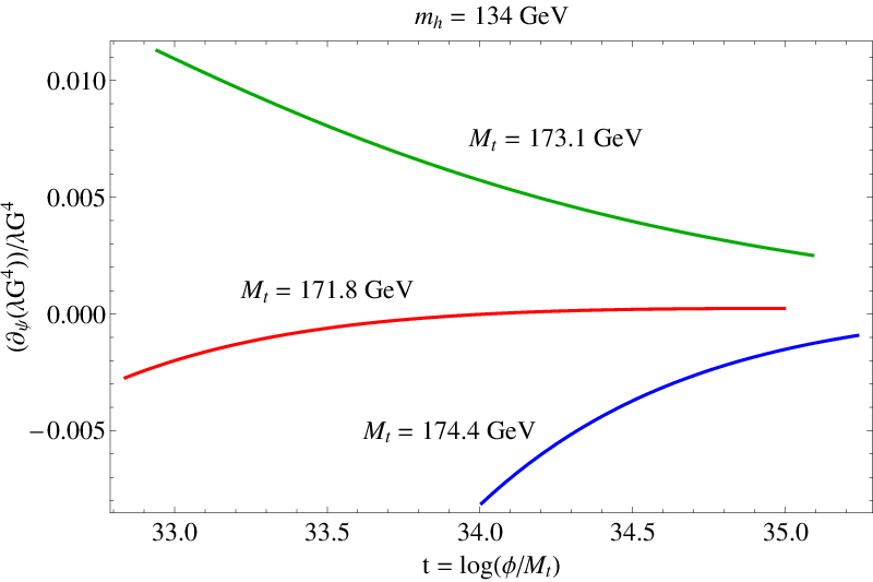
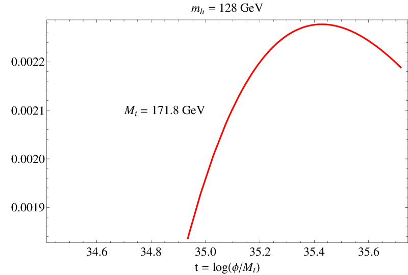
From this approximate expression one obtains a qualitative understanding of how the running of and increases or decreases the classical prediction of the spectral index . The top quark Yukawa coupling plays an important role in the evolution of both and , which in turn determine, in particular, the behavior of the scalar spectral index .
To appreciate the impact of a varying top mass on the vs. curves, consider the relevant leading order terms in the RGE of given by . The second term containing the top Yukawa coupling appears with a negative sign, and so it tries to drive down, whereas the first term with positive sign competes with it and drives up. Since increases with the top mass , the evolution curve gets steeper as we increase . Hence, with larger values of , the spectrum tends to become more red-tilted. Moreover, adds a positive contribution to the spectral index which decreases with increasing . The effect of combined running and is displayed in Fig. 1. In our analysis we employ the RGEs for the SM couplings at two-loop level given in Ref. [5].
The spectral index as a function of the Higgs boson pole mass [15] is depicted in Fig. 2 for three different values of the top quark pole mass: , (the central value of the most recent world average (syst.) [16]) and GeV. As previously noted, the spectral index is quite sensitive to the input value of the top quark pole mass. The constraint on the spectral index with small values, (at - level), given by the combined WMAP plus baryon-acoustic-oscillation and supernovae data [6], implies a lower bound on the Higgs boson mass, which increases as the top quark pole mass is raised as shown in Fig. 2. We note here that for a sufficiently heavy top mass ( GeV), the spectral index acquires values that are smaller than its classical value of . Along with the spectral index and the Higgs boson mass, a precise measurement of the top quark pole mass will be necessary in order to verify the running SM inflation scenario. In the next section we show how seesaw physics can significantly modify some of these conclusions.

Running SM inflation with Type I Seesaw
Type I seesaw is one of the simplest mechanisms for explaining the tiny neutrino masses determined by the solar and atmospheric neutrino oscillation experiments [8]. This is done by introducing two or three right handed neutrinos with masses at the intermediate scale, and by including Dirac Yukawa couplings with left-handed lepton doublets. In the SM supplemented by type I seesaw, at sufficiently high energy scales, the right handed neutrinos are involved in RGEs and therefore modify the running of the SM couplings. We next investigate the effect of type I seesaw on predictions of running SM inflation. Note that for seesaw physics to be relevant the right handed neutrino masses should be smaller than the energy scale of inflation.
Type I Seesaw with One Right Handed Neutrinos
In general, there are several free parameters in type I seesaw associated with the neutrino Dirac Yukawa couplings and right handed neutrino masses, and so it can become quite complicated to analyze the most general case. In order to understand qualitatively the effect on the running SM inflation, we first consider a simplified model with only one right handed neutrino and a single Dirac Yukawa coupling. Through the type I seesaw mechanism, the light neutrino mass is given by
| (16) |
where is the Majorana mass of the right-handed neutrino, and is the Dirac Yukawa coupling. For , the RGEs of the SM couplings are modified due to quantum corrections arising from the right-handed neutrino. For simplicity, we consider only one-loop corrections from this new sector. In this case, the RGEs presented in Appendix of Ref. [5] are modified as follows:
| (17) |
In addition to this modification, we have the RGE for the Dirac Yukawa coupling,
| (18) |

Using these modified RGEs, we analyze running inflation with type I seesaw. For simplicity, we fix the right handed neutrino mass as GeV and show the resultant spectral index for various values of . The limit reproduces the previous results without type I seesaw. Fig. 3 shows the spectral index as a function of Higgs boson mass for various values, with GeV. As expected from the modified RGEs, the effect of type I seesaw is qualitatively analogous to raising the input value of the top quark pole mass in the SM analysis. For larger than a critical value , the spectral index is found to be smaller than the classical prediction.
Type I Seesaw with Three Right Handed Neutrinos
It is certainly interesting to consider more realistic cases so as to reproduce the current neutrino oscillation data. We introduce three generation of right-handed neutrinos and assume a common mass for them, so that the light neutrino mass matrix is given by , where is 33 Dirac Yukawa coupling matrix. This light neutrino mass matrix is diagonalized by a mixing matrix such that
| (19) |
with , where we have assumed, for simplicity, that the Dirac Yukawa matrix is real. We further assume the mixing matrix of the so-called tri-bimaximal form [17],
which is in very good agreement with the current best fit values of the neutrino oscillation data [8].
Let us consider two typical cases for the light neutrino mass spectrum, the hierarchical case and the inverted-hierarchical case. In the hierarchical case, we have
| (24) |
while for the inverted-hierarchical case we choose
| (25) |
with the neutrino oscillation data [8]:
| (26) |
From Eqs. (19)-(26), we can obtain the matrix
| (27) |
as a function of only for the hierarchical and the inverted-hierarchical cases, respectively. For a fixed value of , we obtain a concrete 33 matrix at the scale, which is used as an input in the RGE analysis.


In this more realistic case the modification of RGEs are given by
| (28) |
In addition, we have the RGE for the Dirac Yukawa coupling matrix,
| (29) |
The numerical results are shown in Fig. 4 for both hierarchical and inverted-hierarchical neutrino mass spectra. In both cases, we have obtained qualitatively the same results. Since the seesaw formula requires larger Dirac Yukawa couplings if is raised to reproduce the same light neutrino mass spectrum, the results in the realistic cases are qualitatively consistent with those in the simplified model. The current data of the spectral index sets a lower bound on the Higgs boson mass as a function of the seesaw scale. The bound becomes larger according to the seesaw scale. For a seesaw scale GeV, the scalar spectral index lies below the classical value which is certainly very interesting!

Tensor to Scalar Ratio
With an energy scale during inflation of order , the tensor to scalar ratio turns out to be of order few times , which is about an order of magnitude or so below the detection capability of PLANCK. We show plots of versus in Fig. 5 (without seesaw) and Fig. 6 (including hierarchical seesaw). Detection of at a few percent level can rule out running SM inflation.

Conclusions
Running inflation with a strong non-minimal coupling between the SM Higgs doublet and the Ricci scalar offers an economical scenario of primordial inflation, with the SM Higgs playing the role of the inflaton. With an appropriate choice of the non-minimal coupling, this scenario predicts a scalar spectral index which is consistent with the current data. Very interestingly, there is correlation between the spectral index and the Higgs boson mass, so that this scenario is testable in the near future through synergy between PLANCK and LHC .
Motivated by the neutrino oscillation data, we have investigated the consequences of type I seesaw physics for running SM inflation. We find that the effect of type I seesaw physics at intermediate scales is qualitatively similar to what would happen if the top Yukawa coupling is increased. The current determination by WMAP of the scalar spectral index provides a lower bound on the Higgs boson mass as a function of the neutrino Dirac Yukawa coupling or the right handed neutrino mass. The Higgs mass bound becomes larger as the neutrino Dirac Yukawa coupling or the right handed neutrino mass increases. Therefore, a precision measurement of the spectral index and the Higgs boson mass can reveal not only the existence of running SM inflation but also may have important implications for the seesaw mechanism. Although our main subject is on the running SM inflation in the presence of type I seesaw, it should be noted that the spectral index is found to be drastically changed if we input a sufficiently high top quark pole mass within the error of the current measured value. Thus, a precise measurement of the top quark pole mass also has an impact on testing the running SM inflation scenario.
Acknowledgments
We acknowledge helpful conversations with Andrea de Simone and Ilia Gogoladze and an e-mail correspondence with Misha Shaposhnikov. This work is supported in part by the DOE (MR + QS) under grant # DE-FG02-91ER40626 and by the University of Delaware competitive fellowship (M.R.).
References
- [1] A. H. Guth, Phys. Rev. D 23, 347 (1981); A. D. Linde, Phys. Lett. B 108, 389 (1982); A. J. Albrecht and P. J. Steinhardt, Phys. Rev. Lett. 48, 1220 (1982).
- [2] D. S. Salopek, J. R. Bond and J. M. Bardeen, Phys. Rev. D 40, 1753 (1989), R. Fakir and W. G. Unruh, Phys. Rev. D 41, 1783 (1990), D. I. Kaiser, Phys. Rev. D 52, 4295 (1995) [arXiv:astro-ph/9408044], E. Komatsu and T. Futamase, Phys. Rev. D 59, 064029 (1999) [arXiv:astro-ph/9901127].
- [3] F. L. Bezrukov and M. Shaposhnikov, Phys. Lett. B 659, 703 (2008) [arXiv:0710.3755 [hep-th]]; F. L. Bezrukov, A. Magnin and M. Shaposhnikov, Phys. Lett. B 675, 88 (2009) [arXiv:0812.4950 [hep-ph]]; F. Bezrukov, D. Gorbunov and M. Shaposhnikov, JCAP 0906, 029 (2009) [arXiv:0812.3622 [hep-ph]]; F. Bezrukov and M. Shaposhnikov, JHEP 0907, 089 (2009) [arXiv:0904.1537 [hep-ph]].
- [4] A. O. Barvinsky, A. Y. Kamenshchik and A. A. Starobinsky, JCAP 0811, 021 (2008) [arXiv:0809.2104 [hep-ph]]; A. O. Barvinsky, A. Y. Kamenshchik, C. Kiefer, A. A. Starobinsky and C. Steinwachs, arXiv:0904.1698 [hep-ph]; A. O. Barvinsky, A. Y. Kamenshchik, C. Kiefer, A. A. Starobinsky and C. F. Steinwachs, arXiv:0910.1041 [hep-ph].
- [5] A. De Simone, M. P. Hertzberg and F. Wilczek, Phys. Lett. B 678, 1 (2009) [arXiv:0812.4946 [hep-ph]].
- [6] E. Komatsu et al. [WMAP Collaboration], Astrophys. J. Suppl. 180, 330 (2009) [arXiv:0803.0547 [astro-ph]].
- [7] P. Minkowski, Phys. Lett. B 67, 421 (1977); T. Yanagida, in Proceedings of the Workshop on the Unified Theory and the Baryon Number in the Universe (O. Sawada and A. Sugamoto, eds.), KEK, Tsukuba, Japan, 1979, p. 95; M. Gell-Mann, P. Ramond, and R. Slansky, Supergravity (P. van Nieuwenhuizen et al. eds.), North Holland, Amsterdam, 1979, p. 315; S. L. Glashow, The future of elementary particle physics, in Proceedings of the 1979 Cargèse Summer Institute on Quarks and Leptons (M. Lévy et al. eds.), Plenum Press, New York, 1980, p. 687; R. N. Mohapatra and G. Senjanović, Phys. Rev. Lett. 44, 912 (1980).
- [8] B. T. Cleveland et.al, Astrophys.J. 496 505 (1998); Super-Kamiokande Collaboration, Phys. Lett. B539 179 (2002); Super-Kamiokande Collaboration, Phys. Rev. D71 112005 (2005); M. Maltoni, T. Schwetz, M.A. Tortola, J.W.F. Valle New J.Phys. 6 122 (2004); A. Bandyopadhyay et al, Phys. Lett. B608 115 (2005); G. L. Fogli et al, Prog. Part. Nucl. Phys. 57 742 (2006); For a recent review, see, for example, H. Nunokawa, S. J. Parke and J. W. F. Valle, Prog. Part. Nucl. Phys. 60, 338 (2008).
- [9] G. Lazarides, Q. Shafi and C. Wetterich, Nucl. Phys. B181, 287 (1981); R. N. Mohapatra and G. Senjanović, Phys. Rev. D 23, 165 (1981); M. Magg and C. Wetterich, Phys. Lett. B 94, 61 (1980); J. Schechter and J. W. F. Valle, Phys. Rev. D 22, 2227 (1980).
- [10] R. Foot, H. Lew, X. G. He and G. C. Joshi, Z. Phys. C 44, 441 (1989).
- [11] I. Gogoladze, N. Okada and Q. Shafi, Phys. Rev. D 78, 085005 (2008) [arXiv:0802.3257 [hep-ph]].
- [12] I. Gogoladze, N. Okada and Q. Shafi, Phys. Lett. B 668, 121 (2008) [arXiv:0805.2129 [hep-ph]].
- [13] For a review, see M. Sher, Phys. Rept. 179, 273 (1989), and references therein.
- [14] Note that the energy scale of inflation is of order which, for , lies above the estimated value of cutoff scale . For more discussion of this and related issues see: C. P. Burgess, H. M. Lee and M. Trott, JHEP 0909, 103 (2009) [arXiv:0902.4465 [hep-ph]]; J. L. F. Barbon and J. R. Espinosa, Phys. Rev. D 79, 081302 (2009) [arXiv:0903.0355 [hep-ph]].
- [15] J. R. Espinosa, G. F. Giudice and A. Riotto, JCAP 0805, 002 (2008) [arXiv:0710.2484 [hep-ph]].
- [16] C. Vellidis [CDF Collaboration], arXiv:0910.3392 [hep-ex].
- [17] P. F. Harrison, D. H. Perkins, W. G. Scott, Phys. Lett. B530 167 (2002).