Phase-Mixing and Dissipation of Standing Shear Alfvén waves

Since the discovery of the hot solar corona by Edlén (1943), different theories of coronal heating have been put forward and debated. Heyvaerts & Priest (1983), hereafter HP83, were first to suggest that the phase-mixing of Alfvén waves in coronal plasmas could be a primary mechanism in coronal heating. They showed that the phase-mixing occurs due to inhomogeneity of the local Alfvén phase speed across the background magnetic field. HP83 analytically showed that in both the strong phase-mixing limit and the weak damping approximation, the amplitude of standing Alfvén waves decays with time as $\exp(-At^{3})$ where $A$ is a function of the coordinate corresponding to the inhomogeneous direction ($x$, in this paper). Since then, much analytical and numerical work has been done on the subject. Nocera et al. (1984) studied the phase mixing of propagating Alfvén waves in an inhomogeneous medium. They pointed out if transverse gradients are smeared out as soon as they are formed, this yields to weak phase mixing where damping laws differ from solutions of HP83. Parker (1991) investigated the effect of a density and/or temperature gradient in the direction of vibration of a transverse Alfvén wave. The result was a strong coupling of the waves on different lines of force, producing a coordinated mode that was not subject to simple phase mixing. Hood et al.(1997a) derived a self similar solution of the Alfvén wave phase-mixing equations for heating of coronal holes. They showed that the damping of the waves with height follows the scaling predicted by HP83 at low heights, before switching to an algebraic decay at large heights. Hood et al. (1997b) obtained a simple, self similar solution for the heating of coronal loops by phase mixing. They showed the HP83 model still does work well in a certain class of coronal loops and the phase mixing can supply heating at large Lundquist number at timescales shorter than or comparable with the radiative cooling timescale. Nakariakov et al. (1997) considered the nonlinear excitation of fast magnetosonic waves by phase mixing Alfvén waves in a cold plasma with a smooth inhomogeneity of density across a uniform magnetic field. They suggested this nonlinear process as a possible mechanism of indirect plasma heating by phase mixing through the excitation of fast waves. But Botha et al. (2000) showed that the nonlinear generation of fast modes by Alfvén waves has little effect on classical phase mixing. De Moortel et al. (1999) elaborated the effect of density stratification on phase-mixing. They remarked that when the inhomogeneity in the horizontal direction in the plasma is sufficiently large, so the phase mixing is strong, stratification is unimportant. In the other words due to the rapid phase mixing, energy can be dissipated before the effects of stratification build up. De Moortel et al. (2000) studied the combined effect of a gravitationally stratified density and a radially diverging background magnetic field on phase mixing of Alfvén waves. They found that: i) The efficiency of phase mixing depends strongly on the particular geometry of the configuration. ii) Depending on the value of the scale height the wave amplitudes can damp either slower or faster than in the uniform non-diverging model.

Hood et al. (2002) showed that the amplitude of single pulse and bipolar pulse traveling in the z direction, contrary to infinite wavetrain, have slower algebraic damping of the form $t^{-3/2}$ and $t^{-3}$, respectively, rather than exponential in time. Tsiklauri et al. (2003) cleared that the decay rate of the Alfvénic part of a compressible 3D MHD pulse is affected linearly by the degree of localization of the pulse in the homogeneous transverse direction, but the dynamic of Alfvén waves can still be obtained from the previous 2.5D models, e.g., Hood et al. (2002). Smith et al. (2007) found that in presence of the both density stratification and magnetic field divergence, the enhanced phase mixing mechanism can dissipate Alfvén waves at heights less than half that was predicted by the previous analytical solutions. They stated that if phase-mixing takes place in strongly divergent magnetic fields, it is not necessary to invoke anomalous viscosity in corona.

In the present work, we study the phase mixing of a packet of standing shear Alfvén waves in presence of the both viscous and resistive dissipations. To do this, we numerically solve the linearized MHD equations and obtain the damping time of the oscillations. Our aim is to test the validity of HP83’s damping law for different ranges of the Reynolds and Lundquist numbers. This paper is organized as follows. In Sect. 2, we introduce the basic equations of motion and introduce the model. In Sect. 3, the numerical results are reported, while the conclusions are given in Sect. 4.

The linearized MHD equations for a zero-$\beta$ plasma are:

$\displaystyle\frac{\partial\delta\textbf{v}}{\partial t}=\frac{1}{4\pi\rho_{0}}\{(\nabla\times\delta\textbf{B})\times{\textbf{B}_{0}}+(\nabla\times{\textbf{B}_{0}})\times\delta\textbf{B}\}+\frac{\eta}{\rho_{0}}\nabla^{2}\delta\textbf{v},$

(1)

$\displaystyle\frac{\partial\delta\textbf{B}}{\partial t}=\nabla\times(\delta\textbf{v}\times{\textbf{B}_{0}})+\frac{c^{2}}{4\pi\sigma}\nabla^{2}\delta\textbf{B},$

(2)

where $\delta\textbf{v}$ and $\delta\textbf{B}$ are the Eulerian perturbations in the velocity and magnetic fields; $\rho_{0}$, $\sigma$, $\eta$ and $c$ are the mass density, the electrical conductivity, the viscosity and the speed of light, respectively.

The simplifying assumptions are:

• •

  under coronal conditions gas pressure is negligible (zero-$\beta$);

• •

  the equilibrium density profile is $\rho_{0}=\rho_{0}(x)$;

• •

  there is a constant magnetic field along the $z$ axis, $\textbf{B}_{0}=B_{0}\mathbf{\hat{z}}$;

• •

  there is no initial steady flow inside or outside of the tube;

• •

  the viscous and resistive coefficients, $\eta$ and $\sigma$ respectively, are constants.

To solve Eqs. (1)-(2), following HP83, we neglect the variations in $y$ direction, $\frac{\partial}{\partial y}=0$, and will further assume that the velocity perturbs in $y$ direction. So we choose a solution for the velocity perturbation as

$\displaystyle\delta\textbf{v}(x,z,t)=\delta v_{y}(x,t)\sin(kz){\bf\hat{y}},~~~~~~k=n\pi/L,$

(3)

where $L$ is the length of the loop and $n=(1,2,3,...)$ is the wave number in $z$ direction, respectively. Here the waves are standing because of boundary conditions $\delta\textbf{v}(x,0,t)=\delta\textbf{v}(x,L,t)=0$. Note that HP83 also supposed that the loop is bounded from above an below by boundaries at altitude $z=0$ and $z=L$. It is convenient to work with dimensionless variables $\bar{x}=x/a$, $\bar{z}=z/a$, $\bar{t}=t/\tau_{\rm A}$, $\bar{\rho}_{0}(x)=\rho_{0}(x)/\rho_{00}$, $\delta\bar{\textbf{v}}=\delta\textbf{v}/v_{\rm A_{0}}$ and $\delta\bar{\textbf{B}}=\delta\textbf{B}/B_{0}$. Where $a$ is a typical length scale of density inhomogeneity across the field (i.e. loop radius) and $\tau_{A}=a/v_{\rm A_{0}}$ is a time scale for an Alfvén wave to propagate along the inhomogeneity direction. $\rho_{00}$ and $v_{\rm A_{0}}$ are the plasma density and Alfvén speed at $x=0$, respectively. Finally, Eqs. (1) and (2) in dimensionless form, dropping the ’bars’ for convenience, become

$\displaystyle\frac{\partial\delta v_{y}}{\partial t}=v_{A}^{2}(x)\frac{\partial\delta B_{y}}{\partial z}+\frac{1}{R}\nabla^{2}\delta v_{y},$

(4)

$\displaystyle\frac{\partial\delta B_{y}}{\partial t}=\frac{\partial\delta v_{y}}{\partial z}+\frac{1}{S}\nabla^{2}\delta B_{y},$

(5)

where $v_{\rm A}(x)=\frac{1}{\sqrt{\rho_{0}(x)/\rho_{00}}}$ is the dimensionless form of the Alfvén speed. Also the Reynolds number,

$$R=\Big(\frac{a^{2}\rho_{00}}{\eta}\Big)\Big/\Big(\frac{a}{v_{A_{0}}}\Big),$$

is the ratio of the viscous time-scale to the Alfvén crossing time, and the Lundquist number,

$$S=\Big(\frac{4\pi\sigma a^{2}}{c^{2}}\Big)\Big/\Big(\frac{a}{v_{A_{0}}}\Big),$$

is the ratio of the resistive time-scale to the Alfvén crossing time. Removing $\delta B_{y}$ from Eqs. (4) to (5), and keeping only the first order-terms in $1/R$ and $1/S$ gives

$\displaystyle\frac{\partial^{2}\delta v_{y}}{\partial t^{2}}+k^{2}v_{\rm A}^{2}(x)\delta v_{y}=\Big(\frac{1}{R}+\frac{1}{S}\Big)\nabla^{2}\frac{\partial\delta v_{y}}{\partial t}+T(x,t),$

(6)

where

$\displaystyle T(x,t)=\frac{1}{S}\Big[6\Big(\frac{v_{\rm A}^{\prime}}{v_{\rm A}}\Big)^{2}-2\Big(\frac{v_{\rm A}^{\prime\prime}}{v_{\rm A}}\Big)-4\Big(\frac{v_{\rm A}^{\prime}}{v_{\rm A}}\Big)\frac{\partial}{\partial x}\Big]\frac{\partial\delta v_{y}}{\partial t},$

(7)

where prime indicates a derivative with respect to $x$. It is obvious that the term $T(x,t)$ in Eq. (6) becomes important for high magnetic diffusion plasmas (low S) and in the regions where the Alfvén speed has a large gradient. For more accuracy, in contrast with HP83, we keep this term in our numerical simulations.

Since the dissipation rate is a function of $x$, for calculating the overall damping time, it is suitable to calculate the dimensionless total energy (kinetic energy plus magnetic energy) of the packet per unit of length in the $y$ direction as

$\displaystyle\bar{E}_{\rm tot}(t)=\int_{0}^{2}\Big[\rho_{0}(x)\delta v_{y}^{2}(x,t)+\delta B_{y}^{2}(x,t)\Big]dx,$

(8)

where $\bar{E}_{\rm tot}(t)=\frac{16\pi}{B_{0}^{2}aL}E_{\rm tot}(t)$ and $\delta B_{y}(x,t)$ is calculated from Eq. (5).

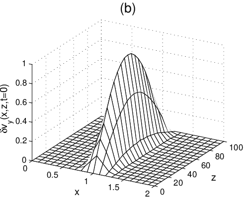
We suppose a functional form of dimensionless Alfvén speed and a Gaussian form of a localized packet of standing Alfvén waves around $x=1$ as

$\displaystyle v_{\rm A}(x)=2+\tanh[\alpha(x-1)],$

(9)

$\displaystyle\delta v(x,z,t=0)=\exp{\Big[-\frac{1}{2}\Big(\frac{x-1}{d}\Big)^{2}\Big]}\sin(kz),$

(10)

where parameter $\alpha$ controls the size of inhomogeneity and $d$ is width of the packet. For $\alpha=2$ and $d=0.1$, the Alfvén speed profile and shape of the initial wave packet given by Eqs. (9) and (10) are plotted in Fig. 1, respectively.

Substituting Eq. (9) in $\omega(x)=kv_{\rm A}(x)$ gives the dimensionless average period of oscillation as

$\displaystyle P_{\rm avg}^{\alpha}=\frac{1}{2}\int_{0}^{2}P(x)dx=\frac{\pi}{k}\int_{0}^{2}\frac{dx}{2+\tanh[\alpha(x-1)]}.$

(11)

As typical parameters for a coronal loop, we assume $L=10^{5}~{\rm km}$, $a=10^{3}~{\rm km}$, $B_{0}=100{~\rm G}$, and $\rho_{00}=2\times 10^{-14}~{\rm gr~cm^{-3}}$. For such a loop, one finds $v_{\rm A_{0}}=2000~{\rm km~s^{-1}}$. Here the loop parameters coincide with the TRACE observations (see Aschwanden et al. 2002; Verwichte et al. 2004). We use a finite difference method to solve Eq. (6), numerically. The evolution of a packet of fundamental standing Alfvén modes is calculated in the range of $0\leq x\leq 2$. To include the dynamical effect of the exterior region, we let the wave packet to evolve up to $x=2$. We suppose that the wave packet never reach at the $x$ boundaries. Hence to avoid any contamination of the solution by the change of boundary values, we fix the boundary conditions. This restricts the time of simulation, but it is still possible to reach the strong phase mixing limit. We choose the boundary and initial conditions as

$\displaystyle\delta v_{y}(x=0,t)=\delta v_{y}(x=2,t)=0,$

(12)

$\displaystyle\delta v_{y}(x,t=0)={\rm e}^{-50(x-1)^{2}},$

(13)

$\displaystyle\frac{\partial\delta v_{y}(x,t)}{\partial t}\Big|_{t=0}=0.$

(14)

There is an upper limit for the time of simulation because we can simulate the evolution until any excitement near the $x$ boundaries could be occurred. The truncation error of numerical results is $\Delta=O(\Delta t^{3})+O(\Delta x^{4})$. We should be aware of choosing suitable spatial step size $\Delta x$, because in the limit of strong phase mixing, large gradients in the $x$ direction are made, so the smaller $\Delta x$ is needed.

Fig. 2 shows contour plots of $\delta v_{y}(x,t)$ in the $x-t$ plane for two different cases with $R=S=10^{4}$ (a) and $R=S=10^{8}$ (b). The white and black colors represent positive and negative values of $\delta v_{y}(x,t)$, respectively. Fig. 2 clears that the defocusing of the packet in the case (a) is large but not in the case (b). This is because of coupling of oscillations in neighboring field lines due to presence of damping terms in the right hand side of Eq. (6). Fig. 3 presents the cross-section cuts along $x=1$, $x=0.6$ and $x=1.4$ for the case (a) with $\alpha=2$ and $d=0.1$. It illustrates that as central regions of the packet decay with time, the neighboring oscillations in the regions with smaller amplitudes, are excited and finally are damped by phase mixing. This means that the packet defocuses along the x direction which is illustrated in Fig. 4. Fig. 5 shows the time evolution of the kinetic energy, magnetic energy and total energy of the packet. Fig. 5 reveals that both the kinetic and magnetic energies of the packet oscillate with time sharply at initial stage of the evolution and then smoothly damped.

Figs. 6-8 show evolution of the packet for the case (b) with $\alpha=2$ and $d=0.1$. Figs. 6-8 in comparing with Figs. 3-5 present that in high Reynolds and Lundquist numbers, i.e. weak damping, the wave packet is damped in developed stage of phase mixing and it’s defocousing is negligible.

From Eq. (8) for $R=S=10^{4}$, $\alpha=2$ and $d=0.1$, we obtain $\tau_{\rm dam}=79.1~\rm s$. From Eq. (11) for $\alpha=2$, the average period of the fundamental mode, $k=\frac{\pi}{100}$, is obtained as $P_{\rm avg}^{\alpha=2}=57.9~\rm s$. Therefore the ratio of the damping time to the average period, $\tau_{\rm dam}/P_{\rm avg}^{\alpha=2}$ for the fundamental mode is 1.4. From Eq. (8) for $R=S=10^{8}$, $\alpha=2$ and $d=0.1$, $\tau_{\rm dam}=1702.6~\rm s$ and $\tau_{\rm dam}/P_{\rm avg}^{\alpha=2}\simeq 29.4$. For $R=S=10^{8}$, if we set $\alpha=4$ and $d=0.05$ then $P_{\rm avg}^{\alpha=4}=62.1\rm~s$, $\tau_{\rm dam}=1072.7\rm~s$ and $\tau_{\rm dam}/P_{\rm avg}^{\alpha=4}\simeq 17.3$. These strong damping times are in agreement with the results observed by Nakariakov et al. (1999) and Wang & Solanki (2004) deduced from the observation of TRACE.

To test the validity of HP83’s damping law in the both weak damping and strong phase mixing limit, we fit the functional form $\exp(-At^{B})$ on the envelope of $\delta v_{y}(x,t)$ at $x=1$. Note that $B=3$ and $A(x)=\frac{1}{6}\nu k^{2}v_{\rm A}^{{}^{\prime}2}(x)$ in HP83, where $\nu=av_{\rm A_{0}}(R^{-1}+S^{-1})$. The numerical results obtained for $A$ and $B$ for different ranges of the Reynolds and Lundquist numbers are tabulated in Table 1. It shows that for $R=S=10^{4}-10^{10}$, the numerical values of $B$ converge to its analytical value but there is one to four order of magnitude difference between the numerical and analytical values of $A$. This returns to keeping the term $T(x,t)$ in Eq. (6) which has been missed in HP83. Table 1 also shows that for $S=10^{12}$ and $R=10^{7}-10^{9}$, the contribution of $T(x,t)$ becomes negligible in Eq. (6) and the numerical values of $A$ and $B$ converge to their corresponding analytical values in HP83’s damping law. Finally one can conclude that the exponential damping law in time of HP83, $\exp(-At^{3})$, is valid for $(R,S)\geq 10^{7}$.

Phase mixing of a packet of standing Alfvénic pulses in fundamental mode is studied. Using a finite difference method, the linearized MHD equations for a zero-$\beta$ plasma are solved, numerically. The damping times of oscillations in presence of the both viscous and resistive dissipations are calculated, numerically. They are in good agreement with the TRACE observations. The exponential damping law in time of HP83, $\exp(-At^{3})$, for the different ranges of the Reynolds and the Lundquist numbers are examined. Our numerical results shows that it is valid for $(R,S)\geq 10^{7}$.

Acknowledgements. This work has been supported financially by Research Institute for Astronomy $\&$ Astrophysics of Maragha (RIAAM), Maragha, Iran.

References

- [1] Aschwanden, M.J., De Pontieu, B., Schrijver, C.J. & Title, A.M., 2002, Sol. Phys., 206, 99
- [2] Botha, G.J.J., Arber, T.D., Nakariakov, V.M. & Keenan, F.P., 2000, A&A, 363, 1186
- [3] De Moortel, I., Hood, A.W., Ireland, J. & Arber, T.D., 1999, A&A, 346, 641
- [4] De Moortel, I., Hood, A.W. & Arber, T.D., 2000, A&A, 354, 334
- [5] Edlén, B., 1943, Z. Astrophysik, 22, 30
- [6] Heyvaerts, J. & Priest, E.R., 1983, A&A, 117, 220
- [7] Hood, A. W., Ireland, J. & Priest, E.R., 1997a, A&A, 318, 957
- [8] Hood, A.W., González-Delgado, D. & Ireland, J., 1997b, A&A, 324, 11
- [9] Hood, A.W., Brooks, S.J. & Wright, A.N., 2002, Proc. R. Soc. Lond. A, 458, 2307
- [10] Nakariakov, V.M., Roberts, B. & Murawski, K., 1997, Sol. Phys., 175, 93
- [11] Nakariakov, V. M., Ofman, L., DeLuca, E.E., Roberts, B. & Davila, J.M., 1999, Science, 285, 862
- [12] Nocera, L., Leroy, B. & Priest, E.R., 1984, A&A, 133, 387
- [13] Parker, E.N., 1991, ApJ, 376, 355
- [14] Smith, P.D., Tsiklauri, D. & Ruderman, M.S., 2007, A&A, 475, 1111
- [15] Tsiklauri, D., Nakariakov, V.M. & Rowlands, G., 2003, A&A, 400, 1051
- [16] Verwichte, E., Nakariakov, V.M., Ofman, L. & Deluca, E.E., 2004, Sol. Phys., 223, 77
- [17] Wang, T.J. & Solanki, S.K., 2004, A&A, 421, L33