Holographic GB gravity in arbitrary dimensions

Preprint: arXiv:0911.4257 [hep-th]
UWO-TH-09/16

Alex Buchel Jorge Escobedo Affiliation: Perimeter Institute for Theoretical Physics, Waterloo, Ontario N2L 2Y5, Canada Affiliation: Department of Applied Mathematics, University of WesternOntario, London, Ontario N6A 5B7, Canada Robert C. Myers Affiliation: Perimeter Institute for Theoretical Physics, Waterloo, Ontario N2L 2Y5, Canada Affiliation: Department of Physics and Astronomy and Guelph-Waterloo Physics Institute,University of Waterloo, Waterloo, Ontario N2L 3G1, Canada Miguel F. Paulos Affiliation: Perimeter Institute for Theoretical Physics, Waterloo, Ontario N2L 2Y5, Canada Aninda Sinha Affiliation: Perimeter Institute for Theoretical Physics, Waterloo, Ontario N2L 2Y5, Canada Affiliation: Department of Applied Mathematics and Theoretical Physics, Cambridge CB3 0WA, UK Michael Smolkin Affiliation: Perimeter Institute for Theoretical Physics, Waterloo, Ontario N2L 2Y5, Canada Affiliation: Racah Institute of Physics, Hebrew University Jerusalem 91904, Israel

Abstract:

We study the properties of the holographic CFT dual to Gauss-Bonnet gravity in general $D\,(\geq 5)$ dimensions. We establish the AdS/CFT dictionary and in particular relate the couplings of the gravitational theory to the universal couplings arising in correlators of the stress tensor of the dual CFT. This allows us to examine constraints on the gravitational couplings by demanding consistency of the CFT. In particular, one can demand positive energy fluxes in scattering processes or the causal propagation of fluctuations. We also examine the holographic hydrodynamics, commenting on the shear viscosity as well as the relaxation time. The latter allows us to consider causality constraints arising from the second-order truncated theory of hydrodynamics.

1 Introduction

The AdS/CFT correspondence [1, 2, 3] or more generally gauge/gravity dualities provide a theoretical framework in which to study (certain) strongly coupled gauge theories. For example, this approach allows for the calculation of transport coefficients for gauge theory plasmas at strong coupling by means of relatively simple supergravity computations, while these calculations are prohibitively complicated by any other conventional methods — for example, see [4, 5, 6]. Recently this topic has been of great interest motivated by the discovery of the strongly coupled quark-gluon plasma (sQGP). In particular, it was found that the ratio of shear viscosity to density entropy of any fluid dual to Einstein gravity is precisely $1/4\pi$ [7, 8]¹¹ 1 Recently this universality has been extended to $T=0$ which is described by extremal black holes in the bulk [9].. Despite the fact that these holographic calculations deal with gauge theories which are quite exotic compared to QCD, this result still seems to come remarkably close to the value measured for the sQGP [10].

Originally it was conjectured that these holographic calculations provided a universal bound: $\eta/s\geq 1/4\pi$ [7]. However, it is now accepted that this conjectured bound is violated in string theory by the effect of higher curvature interactions in the gravitational action. Still the precise string theory constructions where these higher curvature terms are under control only allow for perturbative violations of the bound [11, 12, 13]. It is certainly also of interest to explore situations where finite violations of the bound occur. A useful framework for such explorations was found to be Gauss-Bonnet (GB) gravity [14, 15]. The original studies were made with five-dimensional GB gravity theory which is dual to a four-dimensional CFT but this analysis can easily be extended to any $D\geq 5$ . Some work in this direction already appears in [16, 17]. The present paper provides a comprehensive study of holographic GB gravity in arbitrary dimensions.

An overview of the paper is as follows: We begin with a brief review of Gauss-Bonnet (GB) gravity coupled to a negative cosmological constant in section 2. In section 3, we investigate the AdS/CFT dictionary for these gravitational theories in an arbitrary number of dimensions. In particular, we calculate the central charge $C_{T}$ appearing in the two-point function of the stress tensor and the parameters $t_{2}$ and $t_{4}$ appearing in the energy one-point function describing certain scattering experiments, first proposed in [18]. With these results, we determine the constraints on the GB coupling arising from the requirement that the energy flux in the experiments is everywhere positive. In section 4, we construct the equations of motion for metric perturbations propagating in a black hole background. These equations are then examined in section 5 to study causality violations in the dual CFT. We find that the constraints imposed on the GB coupling to avoid such acausality precisely match the positive energy flux constraints derived in section 3. We examine holographic hydrodynamics for GB gravity in section 6. In particular, by studying the propagation of sound waves in the dual plasma, we derive the relaxation time, as well as the ratio of the shear viscosity to entropy density. Here we also consider causality constraints within the framework of second-order hydrodynamics. We conclude with a brief discussion of our results in section 7. We also have some appendices containing various technical details. In particular, appendix A describes the calculation relating the scattering parameters $t_{2}$ and $t_{4}$ to the couplings $\mathcal{A}$ , $\mathcal{B}$ and $\mathcal{C}$ which determine the three-point function of the stress-energy tensor.

While we were in the final stages of preparing this paper, ref. [19] appeared which also explores causality constraints in Gauss-Bonnet gravity.

2 Gauss-Bonnet gravity

Consider GB gravity in $D\geq 5$ spacetime dimensions, defined by the following action

{I}_{\text{\tiny{GB}}}=\frac{1}{2\ell_{\textrm{\tiny P}}^{D-2}}\int d^{D}x\sqrt{-g}\left[\frac{(D-1)(D-2)}{L^{2}}+R+\frac{L^{2}\,\lambda_{\text{\tiny{GB}}}}{(D-3)(D-4)}\mathcal{X}_{4}\right]\,,

(1)

where

\mathcal{X}_{4}=R_{abcd}R^{abcd}-4R_{ab}R^{ab}+R^{2}\ .

(2)

Of course, this curvature-squared interaction is precisely the Euler density of four-dimensional manifolds and so it does not effect the gravitational equations of motion unless $D\geq 5$ . The solutions describing planar AdS black holes take the form [20]

ds^{2}=\frac{r^{2}}{L^{2}}\left(-\frac{f(r)}{f_{\infty}}\,dt^{2}+\sum_{i=1}^{D-2}(dx^{i})^{2}\right)+\frac{L^{2}}{r^{2}}\,\frac{dr^{2}}{f(r)}\,,

(3)

where $f(r)$ is given by

f_{\pm}(r)=\frac{1}{2\lambda_{\text{\tiny{GB}}}}\left[1\pm\sqrt{1-4\lambda_{\text{\tiny{GB}}}\left(1-\frac{r_{+}^{D-1}}{r^{D-1}}\right)}\ \right]\ .

(4)

In fact, in the following, we will only consider the solutions $f=f_{-}(r)$ as these will be the only ones to correspond to nonsingular black holes in a ghost-free vacuum [21, 22]. Note that in this class of solutions, the horizon appears at $r=r_{+}$ . Using the definition

f_{\infty}=\lim_{r\rightarrow\infty}f(r)=\frac{1-\sqrt{1-4\lambda_{\text{\tiny{GB}}}}}{2\,\lambda_{\text{\tiny{GB}}}}\,,

(5)

we have normalized the coordinates above so that $\lim_{r\rightarrow\infty}g_{tt}/g_{xx}=-1$ . This choice was made to set the speed of light to one in the boundary metric (i.e., in the dual CFT). Further, by setting $r_{+}=0$ , we recover the AdS vacuum metric in Poincaré coordinates. Examining $g_{rr}$ , we can see that the AdS curvature scale $\tilde{L}$ is related to the parameter $L$ in the action as $\tilde{L}^{2}=L^{2}/f_{\infty}$ . In the following, we restrict our discussion to $\lambda_{\text{\tiny{GB}}}<1/4$ since no AdS vacua exist for larger values of $\lambda_{\text{\tiny{GB}}}$ as can be seen, e.g., from eq. (5).

The Hawking temperature of this black hole solution is given by

T=\frac{r_{+}}{4\pi L^{2}}\frac{D-1}{\sqrt{f_{\infty}}}\ .

(6)

The energy and entropy densities are simply calculated as

	$\displaystyle\varepsilon$	$\displaystyle=$	$\displaystyle\frac{D-2}{2\sqrt{f_{\infty}}}\frac{r_{+}^{D-1}}{\ell_{\textrm{\tiny P}}^{D-2}L^{D}}=2\pi\frac{D-2}{D-1}\left(\frac{4\pi\,{f_{\infty}}}{D-1}\right)^{D-2}\,\left(\frac{\tilde{L}}{\ell_{\textrm{\tiny P}}}\right)^{D-2}\,T^{D-1}\ ,$		(7)
	$\displaystyle s$	$\displaystyle=$	$\displaystyle\frac{2\pi}{\ell_{\textrm{\tiny P}}^{D-2}}\left(\frac{r_{+}}{L}\right)^{D-2}=2\pi\left(\frac{4\pi\,{f_{\infty}}}{D-1}\right)^{D-2}\,\left(\frac{\tilde{L}}{\ell_{\textrm{\tiny P}}}\right)^{D-2}\,T^{D-2}\ .$		(8)

Further note that we find that $\varepsilon\propto T^{d}$ and $s\propto T^{d-1}$ as expected for a CFT in $d=D-1$ dimensions (in the absence of a chemical potential). Further, these expressions satisfy the precise relation $\varepsilon=\frac{d-1}{d}Ts$ , again as expected for a conformal plasma.

3 AdS/CFT dictionary

In this section, we develop the dictionary relating the couplings in GB gravity theory (1) to parameters which characterize the dual CFT. Since we are only dealing with the gravitational sector of the AdS theory, we are looking to examine the behaviour of the stress energy tensor of the CFT. So for example, the central charges, $c$ and $a$ , appearing in the trace anomaly are universal parameters characterizing a four-dimensional CFT [23] and can be calculated in holographic context [24]. For GB gravity, these calculations were performed for $d=4$ in [25] and for $d=6$ in [17]. However, while the trace anomaly calculations can be extended to examine CFT’s in higher dimensions, the details change in each dimension and the number of spacetime dimensions must be even. Hence we do not pursue this approach here.

However, there is a “central charge” common to CFT’s in any number of dimensions, $d$ . This is the coefficient characterizing the leading singularity in the two-point function of two stress tensors [26, 27]:²² 2 Here and throughout the following, we are assuming a Minkowski signature for the metric. Note that in eq. (11), $x_{a}=\eta_{ab}x^{b}$ (i.e., $x_{0}=-t$ ).

\langle\,T_{ab}(x)\,T_{cd}(0)\,\rangle=\frac{C_{T}}{x^{2d}}\ {\mathcal{I}}_{ab,cd}(x)\,,

(9)

where

{\mathcal{I}}_{ab,cd}(x)=\frac{1}{2}\left(I_{ac}(x)I_{bd}(x)+I_{ad}(x)I_{bc}(x)\right)-{1\over d}\eta_{ab}\,\eta_{cd}\,,

(10)

and

I_{ab}(x)=\eta_{ab}-2\frac{x_{a}\,x_{b}}{x^{2}}\,.

(11)

This structure is completely dictated by the constraints imposed by conformal symmetry and energy conservation [26, 27]. Of course, in four dimensions, this coefficient is related to the standard central charge $c$ which appears as the coefficient of the (Weyl)² term in the trace anomaly: $C_{T}=(40/\pi^{4})\,c$ . Hence $C_{T}$ will be one of the coefficients which we calculate holographically in the following to establish our AdS/CFT dictionary for GB gravity in general dimensions.

To extend the dictionary further we need to identify additional parameters that play an analogous universal role for CFT’s in any number of spacetime dimensions. With our focus on the stress energy tensor, the obvious next step is to look for universal parameters in the three-point function, as was extensively studied for CFT’s in general dimensions by [26, 27]. There it was shown that conformal symmetry was powerful enough to determine the form of the three-point function up to five constants, which are labeled $\mathcal{A}$ , $\mathcal{B}$ , $\mathcal{C}$ , $\mathcal{D}$ and $\mathcal{E}$ in [26]. Conservation of the stress-energy imposes further constraints which allow us to reduce the number of independent parameters to three with:³³ 3 They also find that this general framework meets exceptions in low dimensions, with two independent parameters in $d=3$ and one, in $d=2$ . These reductions arise because various tensor structures that are independent for $d\geq 4$ are not independent with a small number of dimensions.

	$\displaystyle\mathcal{D}$	$\displaystyle=$	$\displaystyle\frac{d^{2}-4}{2}\,\mathcal{A}+\frac{d+2}{2}\,\mathcal{B}-2d\,\mathcal{C}\,,$
	$\displaystyle\mathcal{E}$	$\displaystyle=$	$\displaystyle(d^{2}-4)\,\mathcal{A}+\frac{d(d+6)}{4}\,\mathcal{B}-\frac{d(d+10)}{2}\,\mathcal{C}\,.$		(12)

Further one finds that Ward identities relate the two- and three-point functions and so $C_{T}$ can be expressed in terms of the parameters characterizing the three-point function [26, 27]:

C_{T}=\frac{\Omega_{d-1}}{2}\,\frac{(d-1)(d+2)\,\mathcal{A}-2\,\mathcal{B}-4(d+1)\,\mathcal{C}}{d(d+2)}\,,

(13)

where $\Omega_{d-1}=2\pi^{d/2}/\Gamma(d/2)$ is the area of a unit ( $d$ –1)-sphere. In fact, one can perform a holographic calculation of the three-point function [28], however, extending these calculations to GB gravity would require an exhaustive and exhausting analysis. Therefore, we choose an indirect route to determining these coefficients in the following.

In particular, we will consider extending the analysis of the energy flux or “energy one-point functions” in [18] for CFT’s in an arbitrary spacetime dimension $d$ . This approach is to consider an “experiment” in which the energy flux was measured at null infinity after a local disturbance was created by the insertion of the stress tensor $\epsilon_{ij}\,T^{ij}$ . The energy flux escaping at null infinity in the direction indicated by the unit vector $\vec{n}$ then takes the form

\langle\mathcal{E}({\vec{n}})\rangle=\frac{E}{\Omega_{d-2}}\left[1+t_{2}\,\left(\frac{\varepsilon^{*}_{ij}\varepsilon_{i\ell}\,n^{j}n^{\ell}}{\varepsilon^{*}_{ij}\varepsilon_{ij}}-\frac{1}{d-1}\right)+t_{4}\,\left(\frac{|\varepsilon_{ij}\,n^{i}n^{j}|^{2}}{\varepsilon^{*}_{ij}\varepsilon_{ij}}-\frac{2}{d^{2}-1}\right)\right]\,,

(14)

where $E$ is the total energy. The structure of this expression is completely dictated by the symmetry of the construction. Hence two coefficients, $t_{2}$ and $t_{4}$ , are constant parameters that characterize the underlying CFT.⁴⁴ 4 One comment is that this general discussion only applies for $d\geq 4$ . It should perhaps be evident that $d=3$ is an exception since in this case, there are not enough spatial directions to consider rotations in the space orthogonal to ${\vec{n}}$ . In fact, we find that the starting point (14) is not quite correct since $\frac{\varepsilon^{*}_{ij}\varepsilon_{i\ell}\,n^{j}n^{\ell}}{\varepsilon^{*}_{ij}\varepsilon_{ij}}=\frac{1}{2}\quad{\rm for}\ d=3\,.$ (15) Hence the most general expression for $d=3$ is simply $\langle\mathcal{E}({\vec{n}})\rangle_{d=3}=\frac{E}{2\pi}\left[1+t_{4}\,\left(\frac{|\varepsilon_{ij}\,n^{i}n^{j}|^{2}}{\varepsilon^{*}_{ij}\varepsilon_{ij}}-\frac{1}{8}\right)\right]\,.$ (16) Note that the (negative) constants appearing in the two factors multiplied by $t_{2}$ and $t_{4}$ were chosen so that these factors contribute zero net flux when integrated over all directions. The negative sign of these constants leads to interesting constraints on the coefficients $t_{2}$ and $t_{4}$ , which we discuss below in section 3.3.

As presented in [25], $t_{2}$ and $t_{4}$ can straightforwardly be determined by a holographic calculation and we generalize these calculations to GB gravity in any number of dimensions in section 3.2 below. As discussed in [18], the energy flux is directly related to the three-point function and hence the two coefficients $t_{2}$ and $t_{4}$ can be determined in terms of $\mathcal{A}$ , $\mathcal{B}$ and $C$ . A lengthy calculation presented in appendix A yields

	$\displaystyle t_{2}$	$\displaystyle=$	$\displaystyle\frac{2(d+1)}{d}\,{(d-2)\,(d+2)\,(d+1)\,\mathcal{A}+3\,d^{\,2}\,\mathcal{B}-4\,d\,(2d+1)\,\mathcal{C}\over(d-1)(d+2)\,\mathcal{A}-2\,\mathcal{B}-4(d+1)\,\mathcal{C}}~,$		(17)
	$\displaystyle t_{4}$	$\displaystyle=$	$\displaystyle-{(d+1)\over d}~{~(d+2)\,(2d^{2}-3d-3)\,\mathcal{A}+2\,d^{\,2}\,(d+2)\,\mathcal{B}-4d\,(d+1)\,(d+2)\,\mathcal{C}\over(d-1)(d+2)\,\mathcal{A}-2\,\mathcal{B}-4(d+1)\,\mathcal{C}}~.$

As further discussed in [18], a nonvanishing $t_{4}$ in a four-dimensional CFT implies the action of the dual gravity theory must contain terms cubic in the Riemann tensor. This analysis readily extends to any number of dimensions and so since such interactions do not appear in the GB gravity action (1) studied here, the holographic CFT must have $t_{4}=0$ . Combined with eq. (17), the vanishing of $t_{4}$ imposes the constraint

(d+2)\,(2d^{2}-3d-3)\,\mathcal{A}+2\,d^{\,2}\,(d+2)\,\mathcal{B}-4d\,(d+1)\,(d+2)\,\mathcal{C}=0

(18)

for the theories studied here.

3.1 Central charge $C_{T}$

First, we perform a holographic calculation of the central charge $C_{T}$ appearing in eq. (9). We follow closely the derivation of the two-point function given in [29]. We consider metric fluctuations propagating in the AdS_d+1 vacuum geometry. It is convenient to write the latter as $ds^{2}=\tilde{L}^{2}/u^{2}(\eta_{ab}\,dx^{a}dx^{b}+du^{2})$ where as above $\tilde{L}^{2}=L^{2}/f_{\infty}$ .⁵⁵ 5 Note that $u=(L\tilde{L})/r$ where $r$ is the radial coordinate used in section 2. We choose a gauge where the perturbation components $\delta g_{uu}=\delta g_{au}=0$ at the AdS boundary. If we write the remaining components as $\delta g_{ab}=\tilde{L}^{2}/u^{2}\,H_{ab}$ , then the (on-shell) quadratic action for $H_{ab}$ reduces to the following boundary term

I_{2}=\frac{\tilde{L}^{d-1}}{8\ell_{\textrm{\tiny P}}^{d-1}}(1-2\lambda_{\text{\tiny{GB}}}f_{\infty})\int_{\partial M}d^{d}x\,u^{1-d}\,H_{ab}\,\partial_{u}H_{ab}\,,

(19)

where the indices are simply contracted with $\delta_{ab}$ . Imposing the boundary conditions

H_{ab}(u=0,{\bf x})=\hat{H}_{ab}({\bf x})\,,

(20)

the full bulk solution for $H_{ab}$ can be written as

H_{ab}(u,{\bf x})=\frac{\Gamma[d]}{\pi^{d/2}\Gamma[d/2]}\,\frac{d+1}{d-1}\int d^{d}x^{\prime}\,\frac{u^{d}}{(u^{2}+|{\bf x}-{\bf x^{\prime}}|^{2})^{d}}\,{\mathcal{I}}_{ab,cd}({\bf x}-{\bf x}^{\prime})\,\hat{H}_{cd}({\bf x^{\prime}})\,,

(21)

where ${\mathcal{I}}_{ab,cd}$ precisely matches the tensor structure appearing in eq. (10). Note that $\delta g_{uu}$ and $\delta g_{au}$ are also nonvanishing in the bulk [29] but we ignore these polarizations because they do not contribute in the quadratic action (19). The quadratic action now becomes

I_{2}=(1-2f_{\infty}\lambda_{\text{\tiny{GB}}})\frac{\Gamma[d+1]}{\pi^{d/2}\Gamma[d/2]}\frac{\tilde{L}^{d-1}}{8\ell_{\textrm{\tiny P}}^{d-1}}\frac{d+1}{d-1}\int d^{d}x\,d^{d}y\,\frac{\hat{H}_{ab}({\bf x})\,{\mathcal{I}}_{ab,cd}({\bf x}-{\bf y})\,\hat{H}_{cd}({\bf y})}{|{\bf x}-{\bf y}|^{2d}}\,.

(22)

Varying the above expression with respect to $\hat{H}_{ab}$ then yields the two-point function of the dual stress tensor and upon comparing with (9), we find

C_{T}=\frac{d+1}{d-1}\frac{\Gamma[d+1]}{\pi^{d/2}\Gamma[d/2]}\,\frac{\tilde{L}^{d-1}}{\ell_{\textrm{\tiny P}}^{d-1}}(1-2f_{\infty}\lambda_{\text{\tiny{GB}}})\,.

(23)

3.2 Holographic calculation of $t_{2}$ and $t_{4}$

In this section, we perform a holographic computation of the energy flux (14). We follow closely the approach presented in [25] and so only sketch the salient steps of the calculation.

We are interested in determining the energy flux

\langle\mathcal{E}(\mathbf{n})\rangle=\frac{\langle 0|\mathcal{O}^{\dagger}\,\mathcal{E}(\mathbf{n})\,\mathcal{O}|0\rangle}{\langle 0|\mathcal{O}^{\dagger}\,\mathcal{O}|0\rangle}\,.

(24)

In the present case, the state is being created by a tensor insertion with $\mathcal{O}\sim\epsilon_{ij}T^{ij}(x)$ where the polarization carries only spatial indices and $\epsilon_{ij}(x)\propto e^{-iEt}$ . Hence we see that this flux is determined by the three- and two-point functions of the stress tensor in the CFT. This expression will depend on the polarization tensor $\epsilon_{ij}$ and the unit vector $n^{i}$ indicating the direction in which the flux is measured. As noted above, the $SO(d-1)$ invariance of the constructions fixes the final result to take the form given in eq. (14).

If we adopt coordinates $x^{\pm}=x^{0}\pm x^{d-1}$ , the energy flux measured at future null infinity in direction specified by $n^{i}$ can be written as

\mathcal{E}(\mathbf{n})=\lim_{x^{+}\to+\infty}\int_{-\infty}^{+\infty}dx^{-}\,(x^{+})^{2}\,\left(1+\frac{x_{\hat{\imath}}x^{\hat{\imath}}}{(x^{+})^{2}}\right)\bigg(T_{+j}^{x}(x^{+},x^{-},\mathbf{n})+T_{-j}^{x}(x^{+},x^{-},\mathbf{n})\bigg)n^{j}\,.

(25)

We have introduced index notation where ${\hat{\imath}}=1,\ldots,d-2$ while $i,j=1,\ldots,d-1$ as usual. The superscript $x$ on the stress tensor simply indicates that these operators are defined in flat space with coordinates $x^{a}$ . This notation is useful because next we introduce new coordinates $y^{a}$ following [18]:

y^{+}=-\frac{1}{x^{+}}\,,\quad y^{-}=x^{-}-\frac{x_{\hat{\imath}}x^{\hat{\imath}}}{x^{+}}\,,\quad y^{{\hat{\imath}}}=\frac{x^{{\hat{\imath}}}}{x^{+}}\,.

(26)

Note that the original Minkowski metric described by $x^{a}$ is conformal to a flat space metric described by $y^{a}$ :

ds^{2}=-dx^{+}dx^{-}+(dx^{\hat{\imath}})^{2}=\frac{-dy^{+}dy^{-}+(dy^{\hat{\imath}})^{2}}{(y^{+})^{2}}\,.

(27)

The utility of transforming to $y^{a}$ is that null infinity, $x^{+}\rightarrow\infty$ , is now mapped to the (hyper)plane $y^{+}=0$ . In this plane, we also have

y^{{\hat{\imath}}}=\frac{n^{{\hat{\imath}}}}{1+n^{d-1}}\,.

(28)

In terms of the new $y$ coordinates, the energy flux (25) becomes

\mathcal{E}({\vec{n}})=\Omega^{d-1}\,\int_{-\infty}^{+\infty}dy^{-}\,T^{y}_{\ --}(y^{+}=0,y^{-},y^{\hat{\imath}})

(29)

with $\Omega\equiv 1/(1+n^{d-1})$ . We have also introduced the $y$ superscript on the stress tensor to indicate the conformally transformed operator:

T^{y}_{ab}=(y^{+})^{2}\,\frac{\partial x^{c}}{\partial y^{a}}\,\frac{\partial x^{d}}{\partial y^{b}}\,T^{x}_{cd}\,.

(30)

To compute $\langle\mathcal{E}(\mathbf{n})\rangle$ holographically, we must turn on graviton perturbations whose boundary values source the appropriate energy-momentum tensor insertions. As the first step [18, 30], we consider the following shockwave background⁶⁶ 6 In this case, $u=L^{4}/r^{2}$ where $r$ is the radial coordinate introduced in section 2.

ds^{2}=\frac{L^{2}}{u}\bigg(\delta(y^{+})W(u,y^{\hat{\imath}})(dy^{+})^{2}-dy^{+}dy^{-}+(dy^{\hat{\imath}})^{2}\bigg)+\frac{L^{2}\,du^{2}}{4f_{\infty}u^{2}}\,.

(31)

In solving for the shockwave profile, the full nonlinear equations of motion for GB gravity reduce to a simple linear equation for $W(u,y^{\hat{\imath}})$ and in fact the curvature-squared terms do not contribute [30, 25]. The solution is chosen with the appropriate asymptotic behaviour to source the operator $\mathcal{E}(n)\simeq\int dy^{-}\,T_{--}$ :

W(u,y^{\hat{\imath}})=N_{W}\,\Omega^{d-1}\,\frac{u^{d/2}}{\bigg(u+(y^{\hat{\imath}}-y^{\prime{\hat{\imath}}})^{2}\bigg)^{d-1}}

(32)

with $y^{\prime{\hat{\imath}}}=n^{{\hat{\imath}}}/(1+n^{d-1})$ as above and $N_{W}$ is a normalisation constant.

It remains to add metric perturbations corresponding to the operators $\mathcal{O}$ in eq. (24). For simplicity, we choose a particular polarization with $\epsilon_{12}=a$ and all other components vanishing. This description applies in the $x$ coordinate system and the dual metric perturbation $\delta g_{ab}=L^{2}/u\,H_{ab}$ would have the boundary condition

H_{x^{1}x^{2}}(u=0)=a\,e^{-iEt}=a\,e^{-i\frac{E}{2}(x^{+}+x^{-})}

(33)

and all other components vanishing. Next we wish to transform to the $y$ coordinates and examine the overlap of the graviton with the shockwave at $y^{+}=0$ . Changing the coordinates, it can be shown [18, 25] that the relevant graviton profile is given by

H_{y^{1}y^{2}}(y^{+}=0,y^{-},y^{\hat{\imath}},u)\simeq\frac{1}{E^{2}}\,e^{-iEy^{-}/2}\ \delta^{d-2}(y^{\hat{\imath}})\,\delta(u-1)\,.

(34)

In general, one also includes additional graviton polarizations to ensure the perturbation is transverse and traceless in the bulk, however, they will not contribute to the three-point function in GB gravity [25].

To find the three-point function, we add this perturbation to the metric (31) and evaluate the action on-shell. We are led to examine terms proportional to $W(H_{y^{1}y^{2}})^{2}$ . After integration by parts and using the equations of motion, the relevant part of the cubic effective action reduces to the following boundary integral:

	$\displaystyle I_{3}=-\frac{1}{8\ell_{\textrm{\tiny P}}^{d-1}}\int d^{d}y\,du\,\sqrt{-g}~H_{y^{1}y^{2}}\,\partial_{-}^{2}H_{y^{1}y^{2}}\,W(u,y^{\hat{\imath}})\,\delta(y^{+})\,\bigg($	$\displaystyle 1-2f_{\infty}\lambda_{\text{\tiny{GB}}}$
		$\displaystyle+\frac{2\lambda_{\text{\tiny{GB}}}f_{\infty}}{(D-3)(D-4)}T_{2}\bigg)\,.$		(35)

In the above expression,

T_{2}\equiv\frac{\partial_{1}^{2}W+\partial_{2}^{2}W-4\,\partial_{u}W}{W}\,.

(36)

After inserting the solution (32) for $W(u,y^{\hat{\imath}})$ , we obtain

T_{2}=2(D-1)(D-2)\left(\frac{n_{1}^{2}+n_{2}^{2}}{2}-\frac{1}{D-2}\right)\,.

(37)

To normalize our result, we must divide by the two-point function $\langle\,T_{12}\,T_{12}\,\rangle$ , which was calculated in the previous section. Upon fixing the normalisation $N_{W}$ of $W(u,y^{\hat{\imath}})$ appropriately, we find that the result takes the desired form (14) with

\langle\mathcal{E}(\theta)\rangle=\frac{E}{\Omega_{d-2}}\left[1+t_{2}\left(\frac{n_{1}^{2}+n_{2}^{2}}{2}-\frac{1}{d-1}\right)\right]

(38)

where the coefficient $t_{2}$ is given by

t_{2}=\frac{4f_{\infty}\lambda_{\text{\tiny{GB}}}}{1-2f_{\infty}\lambda_{\text{\tiny{GB}}}}\,\frac{(D-1)(D-2)}{(D-3)(D-4)}\,.

(39)

Implicitly, as expected, we have also found that $t_{4}=0$ for GB gravity.

3.3 Constraints

Because of the negative constants appearing in eq. (14), it is easy to see that if the coefficients $t_{2}$ and $t_{4}$ become too large, the energy flux measured in various directions will become negative. Avoiding this problem then imposes various constraints, as in [18]. To extract the various distinct constraints, we first fix the unit vector, e.g., $n^{i}=(1,0,0,\cdots)$ . We then organize the polarization tensors $\epsilon_{ij}$ according to their rotational properties under the $SO(d-2)$ group that leaves $n^{i}$ invariant. There are three possibilities and each produces a distinct constraint:

•

Tensor (spin 2), e.g., $\varepsilon_{23}=\varepsilon_{32}=a$ and all other components vanish,

$1-\frac{1}{d-1}\,t_{2}-\frac{2}{d^{2}-1}\,t_{4}\geq 0$ (40)
•

Vector (spin 1), e.g., $\varepsilon_{12}=\varepsilon_{21}=a$ and all other components vanish,

$\left(1-\frac{1}{d-1}\,t_{2}-\frac{2}{d^{2}-1}\,t_{4}\right)+\frac{1}{2}\,t_{2}\geq 0$ (41)
•

Scalar (spin 0), e.g., $\varepsilon_{ij}=a\times{\rm diag}(-(d-2),1,1,\cdots)$ ,

$\left(1-\frac{1}{d-1}\,t_{2}-\frac{2}{d^{2}-1}\,t_{4}\right)+\frac{d-2}{d-1}\left(t_{2}+t_{4}\right)\geq 0$ (42)

These results provide a simple extension to a general dimension $d$ of the constraints for four-dimensional CFT’s derived in [18].

Using the expressions in eq. (17), the above constraints (40), (41) and (42) can be translated to constraints on the parameters $\mathcal{A}$ , $\mathcal{B}$ and $\mathcal{C}$ , e.g., , using eqs. (138) and (139):

$\displaystyle{\rm Tensor:}$	$\displaystyle(d-2)\,(d+2)\,\mathcal{A}+2\,d\,\mathcal{B}-4\,d\,\mathcal{C}\leq 0\,,$	(43)
$\displaystyle{\rm Vector:}$	$\displaystyle(d-2)\,(d+2)\,\mathcal{A}+(3d-2)\,\mathcal{B}-8\,d\,\mathcal{C}\geq 0\,,$	(44)
$\displaystyle{\rm Scalar:}$	$\displaystyle\mathcal{B}-2\,\mathcal{C}\leq 0\,.$	(45)

Note that the three-point couplings obey an additional constraint arising from the unitarity of the CFT. The latter implies that $C_{T}$ is a positive quantity and so from eq. (13), we have

(d-1)(d+2)\,\mathcal{A}-2\,\mathcal{B}-4(d+1)\,\mathcal{C}>0\,.

(46)

This inequality was already assumed in deriving the previous constraints (43–45).

Before turning to the implications for the dual GB gravity, one might consider the results for free fields [27, 26]⁷⁷ 7 The general results for the tensor fields are derived in Appendix B.

$\displaystyle\mathcal{A}$	$\displaystyle=$	$\displaystyle\ \ \frac{1}{\Omega_{d-1}^{3}}\left[\frac{d^{3}}{(d-1)^{3}}n_{s}-\frac{d^{3}}{d-3}\tilde{n}_{t}\right]\,,$
$\displaystyle\mathcal{B}$	$\displaystyle=$	$\displaystyle-\frac{1}{\Omega_{d-1}^{3}}\left[\frac{(d-2)d^{3}}{(d-1)^{3}}n_{s}+\frac{d^{2}}{2}\tilde{n}_{f}+\frac{(d-2)d^{3}}{d-3}\tilde{n}_{t}\right]\,,$	(47)
$\displaystyle\mathcal{C}$	$\displaystyle=$	$\displaystyle-\frac{1}{\Omega_{d-1}^{3}}\left[\frac{(d-2)^{2}d^{2}}{4(d-1)^{3}}n_{s}+\frac{d^{2}}{4}\tilde{n}_{f}+\frac{(d-2)d^{3}}{2(d-3)}\tilde{n}_{t}\right]\,,$

where $\Omega_{d-1}$ is the area of a unit ( $d$ –1)-sphere, as defined below eq. (13). Also $n_{s}$ indicates the number of real conformal scalars and $\tilde{n}_{f}$ is the number of (massless) fermionic degrees of freedom. Hence $\tilde{n}_{f}=2^{\lfloor d/2\rfloor}$ for a massless Dirac fermion in $d$ dimensions — or in the notation of [26], $\tilde{n}_{f}={\rm tr}({\bf 1})$ where tr is the Dirac trace. Finally for the case that $d=2n$ , we have also included the possible contribution of ( $n$ –1)-form potentials, for which the standard free kinetic term is also conformally invariant. Then $\tilde{n}_{t}$ denotes the number of degrees of freedom contributed by these tensors. Generally, for a single ( $n$ –1)-form potential in $d=2n$ , we would have $\tilde{n}_{t}=\Gamma(2n-1)/\Gamma(n)^{2}$ . For example, with $d=4$ , this would just be an Abelian vector field with two degrees of freedom, i.e., $\tilde{n}_{t}=2$ . For $n$ odd, we might also consider constraining the tensor by demanding that the field strength be (anti-)self-dual, in which case the previous result for $\tilde{n}_{t}$ would be multiplied by 1/2.

At this point, it is interesting to evaluate the constraints (43–45) above with these free field results (47) for $\mathcal{A}$ , $\mathcal{B}$ and $\mathcal{C}$

$\displaystyle{\rm Tensor:}$	$\displaystyle(d-2)\,(d+2)\,\mathcal{A}+2\,d\,\mathcal{B}-4\,d\,\mathcal{C}=-\frac{(d^{2}-4)d^{3}}{d-3}\,\tilde{n}_{t}\,,$	(48)
$\displaystyle{\rm Vector:}$	$\displaystyle(d-2)\,(d+2)\,\mathcal{A}+(3d-2)\,\mathcal{B}-8\,d\,\mathcal{C}=\frac{1}{2}(d+2)d^{2}\,\tilde{n}_{f}\,,$	(49)
$\displaystyle{\rm Scalar:}$	$\displaystyle\mathcal{B}-2\,\mathcal{C}=-\frac{(d^{2}-4)d^{2}}{2(d-1)^{3}}\,n_{s}\,.$	(50)

Hence with various combinations of the free fields, we are able to precisely fill out the allowed region that is defined by requiring a positive energy flux in eq. (14).⁸⁸ 8 Momentarily, we are treating $n_{s}$ , $\tilde{n}_{f}$ and $\tilde{n}_{t}$ as continuous variables here. This may be seen as a convenient approximation in the regime where $C_{T}\gg 1$ . As a further note, recall that as discussed in footnote 16, the flux (16) only contains a $t_{4}$ term in $d=3$ . In this case, there are not enough spatial dimensions to establish the tensor constraint (40). The vector and scalar constraints reduce to $-4\leq t_{4}\leq 4\,.$ (51) With $d=3$ , the free field expressions (47) yield $t_{4}=4(n_{s}-\tilde{n}_{f})/(n_{s}+\tilde{n}_{f})$ and hence the free theories again fill the entire range of allowed couplings. For example, with $\tilde{n}_{t}=0$ , we reach the boundary defined by the tensor constraint in eq. (43), i.e., $(d-2)\,(d+2)\,\mathcal{A}+2\,d\,\mathcal{B}-4\,d\,\mathcal{C}=0$ . This boundary surface is mapped out by allowing $n_{s}$ and $\tilde{n}_{f}$ to vary but note that eq. (49) shows that $\tilde{n}_{f}=0$ corresponds precisely to the line where this tensor boundary intersects that set by the vector constraint (44). Similarly, from eq. (50), we see that $n_{s}=0$ corresponds to the intersection of the boundaries set by the tensor (43) and scalar (45) constraints.

Now using the AdS/CFT dictionary established above for GB gravity, we may translate the constraints above to constraints on the GB coupling $\lambda_{\text{\tiny{GB}}}$ . We begin with the constraint $C_{T}>0$ and comparing eq. (23), we find

1-2f_{\infty}\lambda_{\text{\tiny{GB}}}>0\,.

(52)

However, given the definition of $f_{\infty}$ in eq. (5), we find that this constraint is always satisfied – assuming $\lambda_{\text{\tiny{GB}}}<1/4$ , otherwise no AdS vacua exist. This stems from choosing only to consider the branch $f_{-}(r)$ in eq. (4). In fact, the AdS vacua associated with the ‘+’ branch all fail to satisfy the above inequality. This result can be directly related to the ‘ghost’ behaviour of the gravitons in the latter vacua, which is why we disgarded them in section 2. Eq. (52) precisely matches the condition that ensures that the graviton is not a ghost [22].

We now turn to the constraints in eqs. (40–42). Using the expression for $t_{2}$ in eq. (39), as well as $t_{4}=0$ and the definition (5) for $f_{\infty}$ , we arrive at the following constraints:

$\displaystyle{\rm Tensor:}$	$\displaystyle\lambda_{\text{\tiny{GB}}}\leq\frac{(D-3)(D-4)(D^{2}-3D+8)}{4(D^{2}-5D+10)^{2}}\,,$	(53)
$\displaystyle{\rm Vector:}$	$\displaystyle\lambda_{\text{\tiny{GB}}}\geq-\frac{(D+1)(D-3)}{16}\,,$	(54)
$\displaystyle{\rm Scalar:}$	$\displaystyle\lambda_{\text{\tiny{GB}}}\geq-\frac{(3D-1)(D-3)}{4(D+1)^{2}}\,.$	(55)

The most stringent constraints here come from the tensor and scalar channels which require

-\frac{(3D-1)(D-3)}{4(D+1)^{2}}\leq\lambda_{\text{\tiny{GB}}}\leq\frac{(D-3)(D-4)(D^{2}-3D+8)}{4(D^{2}-5D+10)^{2}}\,

(56)

in order that no negative energy fluxes appear in any channel. Similar constraints on the GB coupling arise from demanding that the dual CFT is causal [15]. For five-dimensional GB gravity, it was found that these two sets of constraints were identical [18, 30, 31]. Below we will show that the flux constraints above again match the causality constraints for an arbitrary $D$ .

4 Gauss-Bonnet black hole perturbations

The topics of the two subsequent sections will be the study of causality violations (section 5) and hydrodynamics (section 6) in the CFT’s dual to GB gravity. In both cases, the analysis focuses on examining metric perturbations propagating in the GB black hole background (3). Hence it is useful to outline the general framework and to derive the equations of motion for these perturbations in the present section. To begin, we review the techniques introduced in [32] to study black hole quasinormal modes. The specific background of interest is the GB black hole (3) introduced above. For the following analysis, it is convenient to choose the radial coordinate $u=r_{+}^{2}/r^{2}$ , in which case the metric becomes

ds^{2}=\frac{r_{+}^{2}}{uL^{2}}\left(-\frac{f(u)}{f_{\infty}}\,dt^{2}+\sum_{i=1}^{D-2}dx_{i}^{2}\right)+\frac{L^{2}}{4u^{2}f(u)}du^{2},

(57)

with

f(u)=\frac{1-\sqrt{1-4\lambda_{\text{\tiny{GB}}}(1-u^{\frac{D-1}{2}})}}{2\lambda_{\text{\tiny{GB}}}}

(58)

With this radial coordinate, the horizon is now located at $u=1$ and the boundary at $u=0$ .

Now on this background (57), we wish to study gravitational fluctuations $h_{\mu\nu}$ . The latter are taken to be of the form $h_{\mu\nu}=h_{\mu\nu}(u)e^{-i\omega t+iqz}$ , where we choose the direction $z$ to be the planar coordinate $x^{D-2}$ . As usual according to the AdS/CFT dictionary, these perturbations are dual to stress-energy probes of a finite temperature plasma in the boundary CFT. For simplicity, we restrict to the case where the metric perturbations do not couple to fluctuations of other background fields. The gravitational fluctuations $h_{\mu\nu}$ can be classified according to their transformation properties under the remaining symmetry group $SO(D-3)$ acting in the $x^{\hat{\imath}}$ directions — where ${\hat{\imath}}=1,\dots,{D-3}$ , as in the previous section. Hence, $h_{tt}$ , $h_{tz}$ , $h_{zz}$ , $h_{uu}$ , $h_{tu}$ and $h_{zu}$ transform trivially under these rotations and can be considered as spin 0 perturbations.⁹⁹ 9 Note that the present classification of the probes is identical to that discussed for the states in the scattering processes in section 3.3. Unfortunately here, we cannot refer the spin 0 perturbations as scalar perturbations because this nomenclature clashes with the hydrodynamic terminology – see below. Similarly, $h_{t{\hat{\imath}}}$ , $h_{z{\hat{\imath}}}$ and $h_{u{\hat{\imath}}}$ transform as as spin 1 perturbations and $h_{{\hat{\imath}}\hat{\jmath}}$ transform as spin 2 tensors. Therefore, we have three symmetry channels for gravity perturbations, conventionally referred to as the sound, shear and scalar channels, where the terminology is adopted from the hydrodynamic description of the dual CFT plasma. The equations of motion for fluctuations belonging to different symmetry channels are guaranteed to decouple due to the $SO(D-3)$ symmetry. Following [32], it is convenient to rescale the fluctuations as

H_{tt}=\frac{uL^{2}}{r_{+}^{2}}\frac{f_{\infty}}{f(u)}h_{tt}\,,\quad H_{tz}=\frac{uL^{2}}{r_{+}^{2}}h_{tz}\,,\quad H_{ij}=\frac{uL^{2}}{r_{+}^{2}}h_{ij}\,,\quad H=\sum_{{\hat{\imath}}}H_{{\hat{\imath}}{\hat{\imath}}}=\frac{uL^{2}}{r_{+}^{2}}\frac{h}{(D-3)}\,,

(59)

with $i,j\neq t$ and $h=\sum_{{\hat{\imath}}}h_{{\hat{\imath}}{\hat{\imath}}}$ . In terms of these, we make a particular choice of perturbations for each of the symmetry channels for further study in the following:

Sound channel (spin 0):	$\displaystyle H_{tt},H_{tz},H_{zz},H_{uu},H_{tu},H_{zu},H,$
Shear channel (spin 1):	$\displaystyle H_{tx},H_{zx},H_{ux},$
Scalar channel (spin 2):	$\displaystyle H_{xy}\,.$	(60)

Note that we have renamed $x^{1}=x$ and $x^{2}=y$ for notational convenience. Using the momentum and frequency of the fluctuation, we introduce the following dimensionless quantities

{\swabfamily q}=\frac{q}{2\pi T},\qquad{\swabfamily w}=\frac{\omega}{2\pi T},

(61)

where $T$ is the Hawking temperature (6) of the black hole. Furthermore, we can define the following “gauge-invariant” variables in each of the channels

Sound channel:	$\displaystyle Z_{\text{\tiny{sound}}}\equiv{\swabfamily q}^{2}\frac{f(u)}{f_{\infty}}\,H_{tt}+2{\swabfamily w}\,{\swabfamily q}\,H_{tz}+{\swabfamily w}^{2}H_{zz}+{\swabfamily q}^{2}\left(\frac{f(u)}{f_{\infty}}-\frac{uf^{\prime}}{f_{\infty}}-\frac{{\swabfamily w}^{2}}{{\swabfamily q}^{2}}\right)H,$
Shear channel:	$\displaystyle Z_{\text{\tiny{shear}}}\equiv{\swabfamily q}\,H_{tx}+{\swabfamily w}\,H_{zx},$
Scalar channel:	$\displaystyle Z_{\text{\tiny{scalar}}}\equiv H_{xy}\,.$	(62)

They are gauge-invariant in the sense that they are invariant under the residual infinitesimal diffeomorphisms: $h_{\mu\nu}\to h_{\mu\nu}-\nabla_{\mu}\xi_{\nu}-\nabla_{\nu}\xi_{\mu}$ , where $\xi_{\mu}=\xi_{\mu}(r)e^{-i\omega t+iqz}$ and the covariant derivatives are taken with respect to the background metric (57), which preserve the background metric (57). By first finding the equations of motion obeyed by the rescaled fluctuations $H_{\mu\nu}$ , we will be able to derive second-order differential equations for each of the $Z$ ’s.

To obtain the equations of motion for $H_{\mu\nu}$ , we perturb the black hole metric (3) by $ds^{2}_{pert}$ , which contains an infinitesimal parameter $\epsilon$ . Then, we evaluate the GB Lagrangian as a series in $\epsilon$ and pick up the coefficient of the second-order term. By varying this resulting Lagrangian with respect to each of the fluctuations we obtain the equations of motion of interest. We now present each of the three cases above in turn.

4.1 Scalar channel

The scalar channel is the simplest case as we only need to consider one perturbation, namely

ds^{2}_{\text{pert}}=2\epsilon\,\frac{r_{+}^{2}}{uL^{2}}\left(H_{xy}\,dx\,dy\right)\,.

The resulting equation of motion for the perturbation $Z_{\text{\tiny{scalar}}}\equiv H_{xy}$ is the following:

Z^{\prime\prime}_{\text{\tiny{scalar}}}+\mathcal{C}^{(1)}_{\text{\tiny{scalar}}}\,Z^{\prime}_{\text{\tiny{scalar}}}+\mathcal{C}^{(2)}_{\text{\tiny{scalar}}}\,Z_{\text{\tiny{scalar}}}=0\,,

with the following expressions for the coefficients

\mathcal{C}^{(1)}_{\text{\tiny{scalar}}}=\frac{\mathcal{P}}{uf\mathcal{N}\mathcal{M}}\,,

\mathcal{C}^{(2)}_{\text{\tiny{scalar}}}=\frac{\mathcal{R}}{uf^{2}\mathcal{N}\mathcal{M}}\,.

Here and in the following, the expressions denoted by capital calligraphic letters are expressions that we define in Appendix C in order to present our results as succinctly as possible. These scalar channel equations were already obtained for GB gravity in general spacetime dimensions by [16].

4.2 Shear channel

In the shear channel, we perturb the black hole with

ds^{2}_{\text{pert}}=2\epsilon\,\frac{r_{+}^{2}}{uL^{2}}\left(H_{tx}\,dt\,dx+H_{zx}\,dz\,dx+H_{ux}\,du\,dx\right).

We choose to work in the gauge where $H_{ux}=0$ . The resulting equations that we get from varying the action with respect to $H_{tx}$ , $H_{zx}$ and $H_{ux}$ are, respectively

H^{\prime\prime}_{tx}-\frac{(D-3)}{2}\frac{\mathcal{M}}{u\,\mathcal{N}}\,H^{\prime}_{tx}-\frac{(D-1)^{2}}{16f_{\infty}}\frac{{\swabfamily q}\,\mathcal{M}}{uf\mathcal{N}}\left({\swabfamily q}\,H_{tx}+{\swabfamily w}\,H_{zx}\right)=0,

H^{\prime\prime}_{zx}+\frac{\mathcal{P}}{uf\mathcal{N}\mathcal{M}}\,H^{\prime}_{zx}+\frac{(D-1)^{2}}{16}\frac{{\swabfamily w}}{uf^{2}}\left({\swabfamily q}\,H_{tx}+{\swabfamily w}\,H_{zx}\right)=0,

H^{\prime}_{zx}+\frac{{\swabfamily w}f_{\infty}\mathcal{N}}{{\swabfamily q}f\mathcal{M}}\,H^{\prime}_{tx}=0.

Next, we multiply the first equation by ${\swabfamily q}$ and the second one by ${\swabfamily w}$ , add both equations and, using the third equation, find a differential equation for the gauge-invariant variable $Z_{\text{\tiny{shear}}}\equiv{\swabfamily q}\,H_{tx}+{\swabfamily w}\,H_{zx}$ . The result is

Z^{\prime\prime}_{\text{\tiny{shear}}}+\mathcal{C}^{(1)}_{\text{\tiny{shear}}}\,Z^{\prime}_{\text{\tiny{shear}}}+\mathcal{C}^{(2)}_{\text{\tiny{shear}}}\,Z_{\text{\tiny{shear}}}=0,

(63)

with the following expressions for the coefficients

\mathcal{C}^{(1)}_{\text{\tiny{shear}}}=\frac{-2{\swabfamily w}^{2}f_{\infty}\mathcal{P}\mathcal{N}-(D-3){\swabfamily q}^{2}f^{2}\mathcal{M}^{3}}{2uf\mathcal{M}\mathcal{N}\left({\swabfamily q}^{2}f\mathcal{M}-{\swabfamily w}^{2}f_{\infty}\mathcal{N}\right)},

(64)

\mathcal{C}^{(2)}_{\text{\tiny{shear}}}=\frac{(D-1)^{2}}{16f_{\infty}}\left(\frac{{\swabfamily w}^{2}f_{\infty}\mathcal{N}-{\swabfamily q}^{2}f\mathcal{M}}{uf^{2}\mathcal{N}}\right).

(65)

4.3 Sound channel

Lastly, let us consider the following perturbation in the sound channel

	$\displaystyle ds^{2}_{\text{pert}}=\epsilon\,\frac{r_{+}^{2}}{uL^{2}}\Bigl($	$\displaystyle\frac{f}{f_{\infty}}\,H_{tt}\,dt^{2}+2H_{tz}\,dt\,dz+(D-3)H_{{\hat{\imath}}{\hat{\imath}}}\,(dx^{\hat{\imath}})^{2}+H_{zz}\,dz^{2}+$
		$\displaystyle+2H_{tu}\,dt\,du+2H_{zu}\,dz\,du+H_{uu}\,du^{2}\Bigr)\,.$

Choosing the gauge $H_{tu}=H_{zu}=H_{uu}=0$ , the equations of motion that we obtain from varying the action with respect to $H_{tt}$ , $H_{tz}$ , $H=\sum_{\alpha}H_{\alpha\alpha}$ , $H_{zz}$ , $H_{tu}$ , $H_{zu}$ and $H_{uu}$ , respectively, are the following:

H^{\prime\prime}+\frac{H^{\prime\prime}_{zz}}{(D-3)}+\frac{\mathcal{T}}{uf\mathcal{N}}\,H^{\prime}+\frac{\mathcal{T}}{(D-3)\,uf\mathcal{N}}\,H^{\prime}_{zz}-\frac{(D-1)^{2}}{16f_{\infty}}\frac{{\swabfamily q}^{2}\mathcal{M}}{uf\mathcal{N}}\,H=0,

H^{\prime\prime}_{tz}-\frac{(D-3)}{2}\frac{\mathcal{M}}{u\,\mathcal{N}}\,H^{\prime}_{tz}+\frac{(D-1)^{2}(D-3)}{16f_{\infty}}\frac{{\swabfamily q}\,{\swabfamily w}\,\mathcal{M}}{uf\mathcal{N}}\,H=0,

	$\displaystyle H^{\prime\prime}_{tt}$	$\displaystyle-(D-4)\frac{\mathcal{M}}{\mathcal{N}}\,H^{\prime\prime}-\frac{\mathcal{M}}{\mathcal{N}}\,H^{\prime\prime}_{zz}+\frac{\mathcal{S}}{uf\mathcal{N}}\,H^{\prime}_{tt}-(D-4)\frac{\mathcal{P}}{uf\mathcal{N}^{2}}\,H^{\prime}+$
		$\displaystyle-\frac{\mathcal{P}}{uf\mathcal{N}^{2}}\,H^{\prime}_{zz}-\frac{(D-1)^{2}}{8}\frac{{\swabfamily q}\,{\swabfamily w}\,\mathcal{M}}{uf^{2}\mathcal{N}}\,H_{tz}-\frac{(D-1)^{2}}{16f_{\infty}}\frac{{\swabfamily q}^{2}\mathcal{M}}{uf\mathcal{N}}\,H_{tt}+$
		$\displaystyle-(D-4)\frac{\mathcal{R}}{uf^{2}\mathcal{N}^{2}}\,H-\frac{(D-1)^{2}}{16}\frac{{\swabfamily w}^{2}\mathcal{M}}{uf^{2}\mathcal{N}}\,H_{zz}=0,$

H^{\prime\prime}_{tt}-(D-3)\frac{\mathcal{M}}{\mathcal{N}}\,H^{\prime\prime}+\frac{\mathcal{S}}{uf\mathcal{N}}\,H^{\prime}_{tt}-(D-3)\frac{\mathcal{P}}{uf\mathcal{N}^{2}}\,H^{\prime}-\frac{(D-1)^{2}(D-3)}{16}\frac{{\swabfamily w}^{2}\mathcal{M}}{uf^{2}\mathcal{N}}\,H=0,

		$\displaystyle H^{\prime}+\frac{H^{\prime}_{zz}}{(D-3)}+\frac{{\swabfamily q}}{(D-3){\swabfamily w}}\,H^{\prime}_{tz}+\frac{(D-1)}{2(D-3)}\frac{{\swabfamily q}\,\mathcal{K}}{uf{\swabfamily w}\,\mathcal{N}^{\frac{1}{2}}}\,H_{tz}+\frac{(D-1)}{4}\frac{\mathcal{K}}{uf\mathcal{N}^{\frac{1}{2}}}\,H$
		$\displaystyle+\frac{(D-1)}{4(D-3)}\frac{\mathcal{K}}{uf\mathcal{N}^{\frac{1}{2}}}\,H_{zz}=0,$

H^{\prime}_{tz}+\frac{{\swabfamily q}f}{{\swabfamily w}f_{\infty}}\,H^{\prime}_{tt}-\frac{(D-3){\swabfamily q}f\mathcal{M}}{{\swabfamily w}f_{\infty}\mathcal{N}}\,H^{\prime}-\frac{(D-1)}{4f_{\infty}}\frac{{\swabfamily q}\,\mathcal{K}}{u\,{\swabfamily w}\,\mathcal{N}^{\frac{1}{2}}}\,H_{tt}=0,

	$\displaystyle(D-3)\,H^{\prime}$	$\displaystyle+H^{\prime}_{zz}-\frac{f\mathcal{N}}{\mathcal{V}}\,H^{\prime}_{tt}-\frac{(D-1)^{2}(D-3)}{8(D-2)\mathcal{V}}\left(\frac{{\swabfamily w}^{2}\mathcal{N}}{f}-\frac{{\swabfamily q}^{2}\mathcal{M}}{f_{\infty}}\right)H-\frac{(D-1)^{2}}{8(D-2)}\frac{{\swabfamily w}^{2}\mathcal{N}}{f\,\mathcal{V}}\,H_{zz}+$
		$\displaystyle-\frac{(D-1)^{2}}{8(D-2)}\frac{{\swabfamily q}^{2}\mathcal{N}}{f_{\infty}\mathcal{V}}\,H_{tt}-\frac{(D-1)^{2}}{4(D-2)}\frac{{\swabfamily q}\,{\swabfamily w}\,\mathcal{N}}{f\,\mathcal{V}}\,H_{tz}=0.$

Again, the goal is to use these equations of motion to write a second-order differential equation for the gauge-invariant variable

Z_{\text{\tiny{sound}}}\equiv\frac{{\swabfamily q}^{2}f}{f_{\infty}}\,H_{tt}+2{\swabfamily w}\,{\swabfamily q}\,H_{tz}+{\swabfamily w}^{2}H_{zz}+\frac{{\swabfamily q}^{2}f}{f_{\infty}}\left(1+\frac{(D-1)\mathcal{K}}{2f\mathcal{N}^{1/2}}-\frac{{\swabfamily w}^{2}f_{\infty}}{{\swabfamily q}^{2}f}\right)H.

(66)

After a series of algebraic manipulations, we arrive at the following equation

Z^{\prime\prime}_{\text{\tiny{sound}}}+\mathcal{C}^{(1)}_{\text{\tiny{sound}}}\,Z^{\prime}_{\text{\tiny{sound}}}+\mathcal{C}^{(2)}_{\text{\tiny{sound}}}\,Z_{\text{\tiny{sound}}}=0,

(67)

where the expressions for the coefficients $\mathcal{C}^{(1)}_{\text{\tiny{sound}}}$ and $\mathcal{C}^{(2)}_{\text{\tiny{sound}}}$ are extremely long and are given in Appendix D.

5 Causality constraints

Having obtained the equations of motion for the gauge-invariant variables $Z$ in each of the channels, we now proceed to use them to study causality violation in GB gravity, following [14, 15]. We will focus on the shear and sound channels because the scalar channel was already considered for GB gravity in arbitrary dimensions by [16]. Let us first outline the general strategy behind this approach, which will then be used in each of the channels separately. First, note that in each of the channels, the differential equation for $Z$ has the form

Z^{\prime\prime}(u)+\mathcal{C}^{(1)}Z^{\prime}(u)+\mathcal{C}^{(2)}Z(u)=0.

(68)

The general idea given in [15] consists of introducing a new radial coordinate $\rho$ and rescaling the profile $Z=\psi(u)/B(u)$ to bring this equation (68) into the form of an effective Schrödinger equation,

-\partial^{2}_{\rho}\,\psi+U\,\psi={\swabfamily w}^{2}\psi\,.

(69)

This form can be achieved with $\rho$ and $B$ defined by

	$\displaystyle\frac{d\rho}{du}$	$\displaystyle=$	$\displaystyle-\frac{(D-1)}{4\,u^{1/2}f(u)}\,,$		(70)
	$\displaystyle\frac{d\ln B}{du}$	$\displaystyle=$	$\displaystyle\frac{\mathcal{C}^{(1)}}{2}-\frac{1}{4u}+\frac{(D-1)u^{\frac{D-1}{2}}}{4uf\left(1-2\lambda_{\text{\tiny{GB}}}f\right)}\,.$		(71)

Further, we introduce $\hbar\equiv 1/{\swabfamily q}$ and $\alpha\equiv{\swabfamily w}/{\swabfamily q}$ . Then upon dividing the above equation (69) by ${\swabfamily q}^{2}$ and taking the limit ${\swabfamily q}\to\infty$ (or equivalently $\hbar\to 0$ ) with $\alpha$ fixed, we arrive at

-\hbar^{2}\partial^{2}_{\rho}\,\psi+\left(U^{0}+\hbar^{2}U^{1}+\cdots\right)\psi=\alpha^{2}\psi.

(72)

Note that the effective potential in this equation was obtained by Taylor expanding $U$ in the limit $\hbar\to 0$ . Note that with the above construction, the potential $U^{0}$ only depends on $u$ , $D$ and $\lambda_{\text{\tiny{GB}}}$ , whereas $U^{1}$ and higher order terms may also depend on $\alpha$ . The key point is that in the $\hbar\to 0$ limit, the dominant contribution to the effective potential comes from $U^{0}$ . Hence, for our purposes, it is sufficient to study the equation

-\hbar^{2}\partial^{2}_{\rho}\,\psi+U^{0}\,\psi=\alpha^{2}\psi\,.

(73)

All the preceding is applicable to any of the three channels that we are considering. We will now study the behaviour of equation (73) in each of these channels and give arguments as to what conditions have to be satisifed in order to preserve causality in the dual CFT.

5.1 Shear channel

The leading potential (as $\hbar\to 0$ ) in the shear channel is

U^{0}_{\text{\tiny{shear}}}=\frac{\left[-3+D-2(D-1)\lambda_{\text{\tiny{GB}}}-2(D-5)\lambda_{\text{\tiny{GB}}}f\left(1-\lambda_{\text{\tiny{GB}}}f\right)\right]f}{(D-3)(1-2\lambda_{\text{\tiny{GB}}}f)^{2}f_{\infty}}.

(74)

while the expression for the subleading potential $U^{1}_{\text{\tiny{shear}}}$ is too long to be presented here. With this explicit formula at hand, we can plot the leading potential as a function of $u$ (using (4) and (5)) in the physical region $u\in[0,1]$ . For any $\lambda_{\text{\tiny{GB}}}<1/4$ , we have that $U^{0}_{\text{\tiny{shear}}}(u=0)=1$ and $U^{0}_{\text{\tiny{shear}}}(u=1)=0$ . For small values of $|\lambda_{\text{\tiny{GB}}}|$ , $U^{0}$ is a monotonically decreasing function between the boundary and the horizon. However, as we make $\lambda_{\text{\tiny{GB}}}$ more negative, the potential develops a single maximum between $u=0$ and $u=1$ . This behaviour is illustrated in figure 1.

Refer to caption — Figure 1: (Colour online) Leading potential $U^{0}$ for the Schrödinger-like equation (73) in the shear channel. The blue (solid), green (long dash) and red (small dash) lines correspond to $D=5$ , $6$ and $7$ , respectively. For each dimension, the three potentials correspond to $\lambda_{\text{\tiny{GB}}}=-0.02,-1.5,-3.5$ , from bottom to top. We also show the line $U^{0}=1$ . The behaviour for higher $D$ is similar.

The appearance of a new maximum at some $0<u<1$ implies the existence of quasinormal modes with $\mathop{\rm Re}(\alpha^{2})\simeq>1$ . In turn, this implies that in the limit ${\swabfamily q}\to\infty$ , in which we wrote the Schrödinger equation, $\mathop{\rm Re}({\swabfamily w})/{\swabfamily q}>1$ for these modes, leading to a violation of causality in the dual CFT. Hence to avoid causality violation in this channel, we will impose a bound on $\lambda_{\text{\tiny{GB}}}$ in order to avoid the appearance of a maximum in the potential.

It is clear from the plot in figure 1 that there is some critical value $\lambda_{\text{\tiny{GB}}}^{\text{\tiny{shear}}}$ below which $U^{0}$ exhibits a maximum. To determine the precise value, we first Taylor expand the potential around the boundary $u=0$ obtaining

U^{0}_{\text{\tiny{shear}}}=1-\frac{(D-3)\left(1+\sqrt{1-4\lambda_{\text{\tiny{GB}}}}\right)+8\lambda_{\text{\tiny{GB}}}}{2(D-3)\left(1-4\lambda_{\text{\tiny{GB}}}\right)}\,u^{\frac{D-1}{2}}+\mathcal{O}\left(u^{D-1}\right)\,.

(75)

The sign of the coefficient of the $u^{(D-1)/{2}}$ term will determine whether or not a maximum appears in $U^{0}$ at $u>0$ . The vanishing of this coefficient then determines the critical value of the GB coupling:

\lambda_{\text{\tiny{GB}}}^{\text{\tiny{shear}}}=-\frac{(D+1)(D-3)}{16}\,.

(76)

If the GB coupling is greater than or equal to this value, the potential monotonically decreases to $0$ at $u=1$ . Therefore, we obtain the following lower bound on $\lambda_{\text{\tiny{GB}}}$ which has to be satisfied to preserve causality in the shear channel:

\lambda_{\text{\tiny{GB}}}\geq\lambda_{\text{\tiny{GB}}}^{\text{\tiny{shear}}}=-\frac{(D+1)(D-3)}{16}.

(77)

Note that for $D=5$ and 7, we recover the bounds $\lambda_{\text{\tiny{GB}}}^{\text{\tiny{shear}}}=-3/4$ and –2 which were originally found in [31, 30] and [17], respectively. We also observe that eq. (77) precisely matches the bound (54) that was derived to avoid the appearance of negative energy fluxes in the vector (or spin 1) channel in section 3.3.

As $D$ becomes very large, we see that $\lambda_{\text{\tiny{GB}}}^{\text{\tiny{shear}}}$ is unbounded from below. This is a clear indication that (77) cannot be the correct lower bound for the full GB theory. Indeed, we now show that the correct lower bound comes from the analysis in the sound channel.

5.2 Sound channel

The leading potential (as $\hbar\to 0$ ) in this channel is given by the following expression

$\displaystyle U^{0}_{\text{\tiny{sound}}}=$	$\displaystyle\left[(D-2)\left(1-2\lambda_{\text{\tiny{GB}}}f\right)^{2}f_{\infty}\left(D-3-2(D-1)\lambda_{\text{\tiny{GB}}}-2(D-5)\lambda_{\text{\tiny{GB}}}f\left(1-\lambda_{\text{\tiny{GB}}}f\right)\right)\right]^{-1}$
	$\displaystyle\times\Bigl[(D-2)(D-3)-6(D-1)(D-2)\lambda_{\text{\tiny{GB}}}+12(D-1)^{2}\lambda_{\text{\tiny{GB}}}^{2}+$
	$\displaystyle\quad-2\lambda_{\text{\tiny{GB}}}f\left(1-\lambda_{\text{\tiny{GB}}}f\right)\bigl((D-2)(D-9)+12(D-1)\lambda_{\text{\tiny{GB}}}+$
	$\displaystyle\quad-2(D-3)(D-5)\lambda_{\text{\tiny{GB}}}f\left(1-\lambda_{\text{\tiny{GB}}}f\right)\bigr)\Bigr]f\,.$	(78)

The behaviour of this function is the same as that described in the shear channel, as can be seen in figure 2.

Following the same steps as in the previous case, we obtain the following critical value for the GB coupling

\lambda_{\text{\tiny{GB}}}^{\text{\tiny{sound}}}=-\frac{(D-3)(3D-1)}{4(D+1)^{2}}.

Hence, by the same arguments used before to avoid causality violation in the theory, we get the following lower bound

\lambda_{\text{\tiny{GB}}}\geq\lambda_{\text{\tiny{GB}}}^{\text{\tiny{sound}}}=-\frac{(D-3)(3D-1)}{4(D+1)^{2}}.

(79)

Again, for $D=5$ and 7, we recover $\lambda_{\text{\tiny{GB}}}^{\text{\tiny{sound}}}=-7/36$ and –5/16, as was originally obtained in [31, 30] and [17], respectively. Again comparing to the results in section 3.3, we also find that eq. (79) precisely matches the bound (55) necessary to avoid the appearance of negative energy fluxes in (what was denoted there as) the scalar or spin 0 channel.

Eq. (79) provides a more stringent lower bound than that in the shear channel (77). In particular, when $D$ becomes very large, $\lambda_{\text{\tiny{GB}}}^{\text{\tiny{sound}}}$ is bounded from below by $-3/4$ .

5.3 Scalar channel

For completeness, we present the analysis for the scalar channel, which was already considered in [16]. The expression for the leading potential is in this case

$\displaystyle U^{0}_{\text{\tiny{scalar}}}=$	$\displaystyle\left[(D-4)\left(1-2\lambda_{\text{\tiny{GB}}}f\right)^{2}f_{\infty}\left(D-3-2(D-1)\lambda_{\text{\tiny{GB}}}-2(D-5)\lambda_{\text{\tiny{GB}}}f(1-\lambda_{\text{\tiny{GB}}}f)\right)\right]^{-1}$
	$\displaystyle\times\Bigl[(D-3)(D-4)-2(D-1)(D-6)\lambda_{\text{\tiny{GB}}}-4(D-1)^{2}\lambda_{\text{\tiny{GB}}}^{2}+$
	$\displaystyle\quad-2\lambda_{\text{\tiny{GB}}}f\left(1-\lambda_{\text{\tiny{GB}}}f\right)\bigl[3\left(D(D-7)+14\right)-4(D-1)(2D-7)\lambda_{\text{\tiny{GB}}}+$
	$\displaystyle\quad-2(D-5)(D-7)\lambda_{\text{\tiny{GB}}}f\left(1-\lambda_{\text{\tiny{GB}}}f\right)\bigr]\Bigr]f.$	(80)

The behaviour of this function is shown in figure 3, where we have made use of the bounds found in the shear and sound channel to choose the minimum values that $\lambda_{\text{\tiny{GB}}}$ can take.

We note that, as opposed to the two previous cases, here the single maximum in the potential appears when we increase the value of $\lambda_{\text{\tiny{GB}}}$ . The critical value of the coupling in this channel is given by

\lambda_{\text{\tiny{GB}}}^{\text{\tiny{scalar}}}=\frac{(D-3)(D-4)(D^{2}-3D+8)}{4(D^{2}-5D+10)^{2}}.

Hence, in this case this value gives an upper bound on the GB coupling

\lambda_{\text{\tiny{GB}}}\leq\lambda_{\text{\tiny{GB}}}^{\text{\tiny{scalar}}}=\frac{(D-3)(D-4)(D^{2}-3D+8)}{4(D^{2}-5D+10)^{2}}.

(81)

For $D=5$ and 7, we recover the results $\lambda_{\text{\tiny{GB}}}^{\text{\tiny{scalar}}}=9/100$ and 3/16, first obtained in [15] and [17], respectively. Eq. (79) also precisely matches the upper bound (53) necessary to avoid the appearance of negative energy fluxes in the tensor or (spin 2) channel. Further, we see that as $D$ becomes very large, $\lambda_{\text{\tiny{GB}}}^{\text{\tiny{scalar}}}$ approaches the critical value $\lambda_{\text{\tiny{GB}}}=1/4$ from below.

5.4 Plasma instabilities

To complete this section, let us make some comments on other possible instabilities in the theory. So far, our analysis of the effective Schrödinger equation (73) concerned the possible appearance of superluminal signals in the dual CFT. However, it was noted in [14] that in $D=5$ GB gravity, a new instability arises in the scalar channel at $\lambda_{\text{\tiny{GB}}}=-1/8$ . If one decreases the coupling below this value, the potential $U^{0}_{\text{\tiny{scalar}}}$ develops a negative minimum located right in front of the horizon $u=1$ . Following [33], it was argued that for large ${\swabfamily q}$ , this well supports unstable quasinormal modes. This effect was extensively studied for charged black holes in GB gravity in [16, 34]. In particular, the results of [16] indicate that a similar well develops in the scalar channel of GB gravity for general $D$ , e.g., see figure 4. To obtain the value at which this new instability occurs, expand (80) to around $u=1$

	$\displaystyle U^{0}_{\text{\tiny{scalar}}}=$	$\displaystyle-\frac{\left(1+\sqrt{1-4\lambda_{\text{\tiny{GB}}}}\right)\left((D-3)(D-4)-2(D-1)(D-6)\lambda_{\text{\tiny{GB}}}-4(D-1)^{2}\lambda_{\text{\tiny{GB}}}^{2}\right)}{2(D-4)\left(D-3-2(D-1)\lambda_{\text{\tiny{GB}}}\right)}$
		$\displaystyle\times\,\left(u^{\frac{D-1}{2}}-1\right)+\cdots\,.$

The sign of the coefficient of $\left(u^{(D-1)/2}-1\right)$ will determine whether the potential develops a negative well in front of the horizon. One finds that the negative well develops for [16]

\lambda_{\text{\tiny{GB}}}<-\frac{(D-6)+\sqrt{5D(D-8)+84}}{4(D-1)}.

(82)

Comparing this expression with the lower bound on $\lambda_{\text{\tiny{GB}}}$ obtained in the sound channel (79), we find that this instability arises within the well-behaved regime only for $D=5$ and 6. That is, for

	$\displaystyle D$	$\displaystyle=5:\qquad-\frac{7}{36}\leq\lambda_{\text{\tiny{GB}}}<-\frac{1}{8},$
	$\displaystyle D$	$\displaystyle=6:\qquad-\frac{51}{196}\leq\lambda_{\text{\tiny{GB}}}<-\sqrt{\frac{3}{50}}$		(83)

the GB theory is dual to a well-behaved CFT, but the plasma still seems to exhibit instabilities corresponding to unstable quasinormal modes in the black hole background. Given that these modes have large momentum, it seems that the instability causes the homogeneous CFT plasma to “clump” into an inhomogeneous configuration. However, for $D\geq 7$ (or $d\geq 6$ ), the values given by (82) are ruled out by the lower bound (79) and so no such scalar channel instabilities arise in the dual CFT’s (which are not already pathological for other reasons).

Of course, one should also examine the shear and sound channels for similar instabilities. In [31], it was observed for $D=5$ that the shear channel does not produce any new instabilities. Similarly, examining the potential (74) the same result applies for arbitrary values of $D$ . It was also observed in [31] that in $D=5$ the sound channel can develop instabilities for $\lambda_{\text{\tiny{GB}}}>1/8$ . Hence, this effect only occurs outside of the physical regime, i.e., $\lambda_{\text{\tiny{GB}}}\leq 9/100$ . For $D\geq 6$ we examine the potential (78) for the possible appearence of a negative well. We find $U^{0}_{\text{\tiny{sound}}}\geq 0$ everywhere in the range $1\geq u\geq 0$ for $D\geq 6$ . Hence if we restrict the GB coupling, as in eq. (56), to produce a physically well-behaved CFT, the shear and sound channels do not produce any new instabilities for a homogeneous plasma.

6 Second-order hydrodynamics

Hydrodynamics of relativistic fluids is discussed in [4, 35]. Here we summarize a few relevant results for our computations. Let us consider a $(D-1)$ -dimensional conformal fluid, as is appropriate for the CFT dual of $D$ -dimensional GB gravity. The dynamics of the long wavelength fluctuations can be organized in terms of a derivative expansion. In particular, in the absence of any conserved charges, the dynamics of the hydrodynamic modes is simply governed by the conservation of the stress-energy tensor: $\nabla_{a}T^{ab}=0$ . The latter includes both the equilibrium part, involving the local energy density $\varepsilon$ and pressure $P$ , and a dissipative part $\Pi^{ab}$

T^{ab}=\varepsilon\,u^{a}u^{b}+P\Delta^{ab}+\Pi^{ab}\,,

(84)

where $\Delta^{ab}=g^{ab}+u^{a}u^{b}$ and $u^{a}$ is the local four-velocity of the fluid, with $u^{a}u_{a}=-1$ . For a conformal fluid, we also have the restriction that the trace of the stress tensor must vanish, i.e., $T^{a}{}_{a}=0$ . In the equilibrium contribution above, this requires that $P=\varepsilon/(D-2)$ .

The dissipative term can be written as an infinite series expansion in velocity gradients and curvatures (for a fluid in a curved background), where the coefficients in this expansion are the transport coefficients of the fluid. At first order for a conformal fluid, one has

\Pi^{ab}_{1}=-\eta\,\sigma^{ab}\,,

where

\sigma^{ab}=2\nabla^{\langle a}u^{b\rangle}\equiv\Delta^{ac}\Delta^{bd}\left(\nabla_{c}u_{d}+\nabla_{d}u_{c}\right)-\frac{2}{D-2}\Delta^{ab}\Delta^{cd}\nabla_{c}u_{d}\,.

Implicitly here, we have used the condition that $T^{a}{}_{a}=0$ to eliminate any bulk viscosity contribution. Hence the only nonvanishing transport coefficient appearing at this order is the shear viscosity $\eta$ . Of course, if we truncate the hydrodynamic equations to include only this “Newtonian” first-order term, there are superluminal modes propagating in the fluid [36]. One can try to avoid this problem by going to next order in the expansion [37]. In general for a conformal fluid, five new transport coefficients will appear in the second-order term $\Pi^{ab}_{2}$ . However, there is only one contribution which is independent of both the vorticity and background curvature, as well as linear,

\Pi^{ab}_{2}=\eta\tau_{\Pi}\left[{}^{\langle}u\cdot\nabla\sigma^{ab\rangle}+\frac{1}{D-2}\sigma^{ab}\left(\nabla\cdot u\right)\right]\,.

The additional transport coefficient above is the relaxation time $\tau_{\Pi}$ and this linear term is sufficient to examine the question of causality within the hydrodynamic regime [38].

In [4], the authors studied linearized fluctuations of the second-order hydrodynamics of conformal fluids and found the following results:

$\bullet$ Shear channel

The dispersion relation in the shear channel was found to be

-{\swabfamily w}^{2}\tau_{\Pi}T-\frac{i\,{\swabfamily w}}{2\pi}+{\swabfamily q}^{2}\frac{\eta}{s}=0,

(85)

where ${\swabfamily w}$ and ${\swabfamily q}$ are defined in eq. (61). We are interested in the hydrodynamic limit in which ${\swabfamily w},{\swabfamily q}\to 0$ , with ${\swabfamily w}/{\swabfamily q}$ kept fixed. In this limit, the dispersion relation (85) yields the following Taylor series solution

{\swabfamily w}=-2\pi i\,\frac{\eta}{s}\,{\swabfamily q}^{2}-8\pi^{3}i\,\tau_{\Pi}T\,\frac{\eta^{2}}{s^{2}}\,{\swabfamily q}^{4}+\mathcal{O}({\swabfamily q}^{6}).

(86)

Note that we have discarded a solution where ${\swabfamily w}$ remains finite as ${\swabfamily q}\to 0$ , hence lying beyond the hydrodynamic regime — see [4]. The wave-front speed with which disturbances propagate out from a discontinuity in any initial data is governed by [39]

v_{\text{\tiny{shear}}}^{\text{\tiny{front}}}\equiv\lim_{|{\swabfamily q}|\to\infty}\frac{\mathop{\rm Re}({\swabfamily w})}{{\swabfamily q}}=\sqrt{\frac{\eta}{\tau_{\Pi}T\,s}}\,.

(87)

Thus, requiring causality to be preserved in this channel of a conformal fluid imposes the following bound [31]

\tau_{\Pi}T\geq\frac{\eta}{s}\,.

(88)

$\bullet$ Sound channel

The dispersion relation in the sound channel was found to be

-{\swabfamily w}^{3}\tau_{\Pi}T-\frac{i\,{\swabfamily w}^{2}}{2\pi}+{\swabfamily w}\,{\swabfamily q}^{2}c_{s}^{2}\tau_{\Pi}T+{\swabfamily w}\,{\swabfamily q}^{2}\frac{2(D-3)}{(D-2)}\frac{\eta}{s}+\frac{i\,{\swabfamily q}^{2}c_{s}^{2}}{2\pi}=0,

(89)

where $c_{s}$ is the speed of sound, which in any conformal fluid is a constant

c_{s}^{2}=\frac{1}{D-2}\,.

(90)

At small momentum ${\swabfamily q}$ , the Taylor series solution to the above equation corresponding to the sound wave is

{\swabfamily w}=c_{s}\,{\swabfamily q}-2\pi i\,\Gamma T\,{\swabfamily q}^{2}+\frac{4\pi^{2}}{c_{s}}\Gamma T\left(c_{s}^{2}\tau_{\Pi}T-\frac{\Gamma T}{2}\right){\swabfamily q}^{3}+\mathcal{O}({\swabfamily q}^{4}),

(91)

where

\Gamma T=\frac{D-3}{D-2}\,\frac{\eta}{s}\,.

(92)

Note that we have only written one of the three solutions to (89). The second solution corresponds to waves propagating in the opposite direction, i.e., replace ${\swabfamily q}$ with $-{\swabfamily q}$ in eq. (91). The third solution again lies beyond the regime of validity of hydrodynamics. Given eq. (91), we have

v_{\text{\tiny{sound}}}^{\text{\tiny{front}}}\equiv\lim_{|{\swabfamily q}|\to\infty}\frac{\mathop{\rm Re}({\swabfamily w})}{{\swabfamily q}}=\sqrt{c_{s}^{2}+\frac{2(D-3)}{(D-2)}\frac{\eta}{s}\frac{1}{\tau_{\Pi}T}}\,.

(93)

Hence, causality in this channel imposes the following bound

\tau_{\Pi}T\geq 2\frac{\eta}{s}.

(94)

It is quite interesting that despite the explicit appearance of $D$ in eq. (93), the bound (94) is independent of the dimension and takes the same simple form as originally found for $D=5$ in [31].

We see that in both channels considered above, the wave-front speed of the linearized fluctuations diverges as the relaxation time $\tau_{\Pi}$ goes to zero. Notice also that the front velocity in the sound channel is always larger than that in the shear channel. Therefore, the bound (94) provides a stronger constraint on the transport coefficients. As emphasized in [31], the constraints (88) and (94) arise when considering linearized modes outside the regime of validity of hydrodynamics. Hence, these constraints must not be regarded as fundamental, as they merely indicate where a certain approximate framework describing the conformal fluid becomes problematic.

6.1 Holographic Gauss-Bonnet hydrodynamics

Next we would like to apply the now standard techniques [40, 4] of the AdS/CFT framework to calculate the transport coefficients $\eta$ and $\tau_{\Pi}$ for the CFT’s dual to GB gravity in an arbitrary spacetime dimension. The shear viscosity for GB gravity in $D=5$ was originally calculated in [14], however, these calculations are easily extended to GB gravity in any dimension [14, 16]. Their result is

\frac{\eta}{s}=\frac{1}{4\pi}\left[1-\frac{2(D-1)}{(D-3)}\lambda_{\text{\tiny{GB}}}\right]\,,

(95)

where the entropy density $s$ is given in eq. (8). We reproduce this result with our analysis of the sound waves below.

Hence it remains for us to calculate the relaxation time $\tau_{\Pi}$ . For this purpose, we must solve the equation of motion (67), which describes the propagation of sound waves in the CFT plasma dual to GB gravity. This allows us to obtain expressions that can be compared to those presented in the previous subsection. First, we make the following ansatz for the solution near the horizon

Z_{\text{\tiny{sound}}}=(1-u^{\frac{D-1}{2}})^{\beta},

where there could be an overall coefficient independent of $u$ , which is not relevant for our discussion. If we replace this ansatz into (67), we readily obtain the following two solutions

\beta=\pm\frac{i{\swabfamily w}}{2},

with the negative sign satisfying the correct infalling boundary condition at the horizon. Let us now focus on the hydrodynamic limit, where ${\swabfamily w}$ , ${\swabfamily q}\rightarrow 0$ with $\frac{{\swabfamily w}}{{\swabfamily q}}$ kept fixed. We will write our solution as a series in ${\swabfamily q}$ and then solve eq. (67) perturbatively. The horizon boundary condition implies that we can write our solution as

Z_{\text{\tiny{sound}}}=(1-u^{\frac{D-1}{2}})^{-\frac{i{\swabfamily w}}{2}}\left(z_{0}(u;{\swabfamily w},{\swabfamily q})+i{\swabfamily q}\,z_{1}(u;{\swabfamily w},{\swabfamily q})+{\swabfamily q}^{2}z_{2}(u;{\swabfamily w},{\swabfamily q})+\mathcal{O}({\swabfamily q}^{3})\right),

(96)

where at the horizon $\lim_{u\to 1}z_{i}(u;{\swabfamily w},{\swabfamily q})=\delta^{0}_{i}$ with $i=0,1,2$ . Further each of the $z_{i}(u;{\swabfamily w},{\swabfamily q})$ should only depend on the ratio ${\swabfamily w}/{\swabfamily q}$ which implies a scaling invariance

z_{i}(u;\mu\,{\swabfamily w},\mu\,{\swabfamily q})=z_{i}(u;{\swabfamily w},{\swabfamily q})

(97)

for any $\mu$ . In this expansion, we have only written terms to the order necessary to identify the sound wave dispersion relation (91), which is obtained by imposing the Dirichlet boundary condition on $Z_{\text{\tiny{sound}}}$ at the asymptotic boundary

\lim_{u\to 0}Z_{\text{\tiny{sound}}}=0\,.

(98)

By comparing the terms of the dispersion relation at each order in ${\swabfamily q}$ , we will be able to identify the expressions for the conformal sound speed $c_{s}$ (the leading order), the shear viscosity to entropy ratio $\eta/s$ (the first order) and the relaxation time $\tau_{\Pi}$ (the second order). The analysis is greatly simplified by adopting a new radial coordinate

x\equiv\sqrt{1-4\lambda_{\text{\tiny{GB}}}(1-u^{\frac{D-1}{2}})}.

(99)

With this radial coordinate, the horizon and asymptotic boundary conditions become

	$\displaystyle\lim_{x\to 1}z_{i}(x;{\swabfamily w},{\swabfamily q})$	$\displaystyle=\delta^{0}_{i}\qquad\text{(horizon)},$
	$\displaystyle\lim_{x\to(1-4\lambda_{\text{\tiny{GB}}})^{1/2}}Z_{\text{\tiny{sound}}}$	$\displaystyle=0\qquad\text{(boundary)}.$		(100)

6.1.1 Speed of sound

Solving eq. (67) perturbatively, the leading order term gives a second-order differential equation for $z_{0}(x)$ . We will not write the explicit equation here, but merely state its solution,

z_{0}=\frac{{\swabfamily q}^{2}\left[(D-5)x^{2}+4x-(D-1)\left(1-4\lambda_{\text{\tiny{GB}}}\right)\right]-8\left(D-2\right)f_{\infty}{\swabfamily w}^{2}\lambda_{\text{\tiny{GB}}}\,x}{4\left[(D-1){\swabfamily q}^{2}-2\left(D-2\right)f_{\infty}{\swabfamily w}^{2}\right]\lambda_{\text{\tiny{GB}}}x}\,.

(101)

By imposing the Dirichlet boundary condition (100) and solving for w, we find the expected dispersion relation

{\swabfamily w}=\frac{1}{\sqrt{D-2}}\,{\swabfamily q}\,.

(102)

Of course, the factor $1/\sqrt{D-2}$ is precisely the speed of sound (90) for a conformal fluid in $D-1$ dimensions.

6.1.2 Shear viscosity-to-entropy ratio

To first order in ${\swabfamily q}$ we obtain a second-order differential equation for $z_{1}(x)$ , which involves the previously found $z_{0}(x)$ . This equation is even more involved than that for $z_{0}(x)$ . To proceed we make the following ansatz for the solution $z_{1}=\left({\swabfamily w}/{\swabfamily q}\right)\,z_{0}(x)\,F(x)$ . Again, it is not very illuminating to write the resulting equation and so we simply give its solution

$\displaystyle F(x)=$	$\displaystyle\frac{1}{{\swabfamily q}^{2}\left[(D-5)x^{2}+4x-(D-1)\left(1-4\lambda_{\text{\tiny{GB}}}\right)\right]-8\left(D-2\right)f_{\infty}{\swabfamily w}^{2}\lambda_{\text{\tiny{GB}}}\,x}\times$
	$\displaystyle\Biggl[\left[{\swabfamily q}^{2}\left[(D-5)x^{2}+4x-(D-1)\left(1-4\lambda_{\text{\tiny{GB}}}\right)\right]-8\left(D-2\right)f_{\infty}{\swabfamily w}^{2}\lambda_{\text{\tiny{GB}}}\,x\right]\times$
	$\displaystyle\biggl[\sqrt{\frac{(D-1)(1-4\lambda_{\text{\tiny{GB}}})}{4(D-5)}}\arctan\left(\frac{\sqrt{(D-1)(D-5)(1-4\lambda_{\text{\tiny{GB}}})}}{(D-1)(1-4\lambda_{\text{\tiny{GB}}})+(D-5)x}(1-x)\right)+$
	$\displaystyle+\frac{1}{2}\ln\left(\frac{1+x}{2}\right)-\frac{(D-1)(1-4\lambda_{\text{\tiny{GB}}})}{4(D-5)}\ln\left(\frac{(D-5)x^{2}+(D-1)(1-4\lambda_{\text{\tiny{GB}}})}{2(D-3)-4(D-1)\lambda_{\text{\tiny{GB}}}}\right)\biggr]+$
	$\displaystyle-4{\swabfamily q}^{2}x(1-x)\left((D-3)-2(D-1)\lambda_{\text{\tiny{GB}}}\right)\Biggr]\,.$	(103)

Note that while at first sight it might seem that this result is not well-behaved at $D=5$ , taking the limit $D\to 5$ carefully, recovers the results obtained in [31] — in taking this limit, one should recall that $\lambda_{\text{\tiny{GB}}}<1/4$ . Given this general solution (103), we can impose the Dirichlet boundary condition at infinity and solve for ${\swabfamily w}$ , obtaining the following dispersion relation up to second-order in q

{\swabfamily w}=\frac{1}{\sqrt{D-2}}{\swabfamily q}-i\frac{(D-3)}{2(D-2)}\left[1-\frac{2(D-1)}{(D-3)}\lambda_{\text{\tiny{GB}}}\right]{\swabfamily q}^{2}.

By comparing to eqs. (91) and (92), we see that the factor in brackets in the second-order coefficient is essentially the ratio of the shear viscosity to entropy density with

\frac{\eta}{s}=\frac{1}{4\pi}\left[1-\frac{2(D-1)}{(D-3)}\lambda_{\text{\tiny{GB}}}\right].

(104)

Of course, this precisely reproduces the result found previously in [14, 16].

6.1.3 Relaxation time and causality violation

To second order in ${\swabfamily q}$ we obtain a differential equation for $z_{2}(x)$ , involving $z_{0}(x)$ and $z_{1}(x)$ . Unfortunately, we were only able to solve this equation numerically.¹⁰¹⁰ 10 The details of numerical calculations will not be presented here, but are available from the authors upon request. Naturally, this means that we are not able to obtain general expressions for arbitrary values of $D$ . Here we present numerical results for $D=5,6,7,8$ but these are indicative of the behaviour for higher dimensions as well. Note that the constraint (94) to avoid causality violations requires

\tau_{\Pi}T-2\frac{\eta}{s}\geq 0.

We show the results of our numerical computations for this quantity in figure 5. We see that for $D>6$ , causality does not impose an upper bound on the GB coupling, however, we still require $\lambda_{\text{\tiny{GB}}}<1/4$ as was assumed from the very beginning of the discussion. From these numerical results, we find the following bounds for having causal second-order hydrodynamics,

$\displaystyle D$	$\displaystyle=5:\qquad-0.711\leq\lambda_{\text{\tiny{GB}}}\leq 0.113,$
$\displaystyle D$	$\displaystyle=6:\qquad-1.7\leq\lambda_{\text{\tiny{GB}}}\leq 0.171,$
$\displaystyle D$	$\displaystyle=7:\qquad-3.1\leq\lambda_{\text{\tiny{GB}}}<0.25,$
$\displaystyle D$	$\displaystyle=8:\qquad-5.0\leq\lambda_{\text{\tiny{GB}}}<0.25.$	(105)

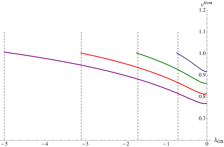
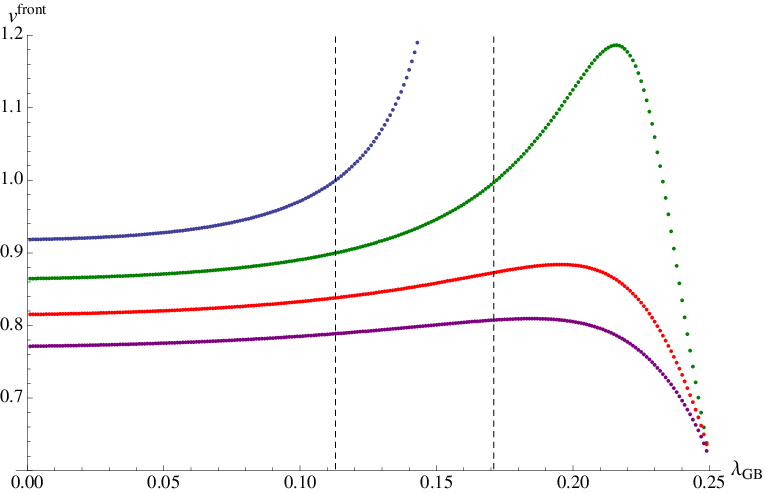
Note that we do not quote the bounds in higher dimensions with the same accuracy because the numerical analysis became more unstable for large values of $D$ . In figure 6, we also present the behaviour of the front velocity (93) in the sound channel for these various cases.

7 Discussion

In this present paper, we have made a broad study of holographic GB gravity in arbitrary dimensions. The first step was to construct the AdS/CFT dictionary which applies for arbitrary $D$ in section 3. There are two dimensionless parameters which characterize GB gravity, i.e., the ratio of the AdS curvature scale to Planck scale, $\tilde{L}/\ell_{\textrm{\tiny P}}$ , and the GB coupling, $\lambda_{\text{\tiny{GB}}}$ . Since we are only dealing with the gravitational sector of the AdS theory, these parameters are naturally related to CFT parameters which determine the behaviour of the $n$ -point functions of the stress-energy tensor. So for example, using eqs. (23) and (39), we can translate the gravitational parameters to expressions in terms of the central charge $C_{T}$ and the scattering parameter $t_{2}$ . Alternatively, they could be expressed in terms of the three-point couplings $\mathcal{A},\mathcal{B},\mathcal{C}$ using eqs. (13) and (17) (keeping in mind the constraint (18)). Given the results of section 3, one can express any physical quantities, e.g., $\eta/s$ , entirely in terms of parameters appearing in the CFT. This is, of course, an essential step in the program of using holographic models to characterize the properties of the quark-gluon plasma [41].

Using these results, an interesting observation can be made with regards to the relation between the central charge $C_{T}$ appearing in the two-point function and the “central charge” characterizing the entropy density. That is, one can use the entropy density of a CFT in $d$ dimensions to provide an alternative definition of a central charge: $C_{S}\propto s/T^{d-1}$ . In two dimensions, $C_{T}$ and $C_{S}$ are related by a simple numerical factor. However, there is no evidence of any simple relation for strongly coupled CFT’s in higher dimensions, e.g., see [42, 43]. This alternative central charge was recently considered for CFT’s dual to Einstein gravity in [44] and here we extend the discussion to consider GB gravity in an arbitrary number of dimensions. First we adopt the normalization of [44] in defining $C_{S}$ as

C_{S}\equiv\frac{d+1}{d-1}\left(\frac{d}{2\pi^{3/2}}\right)^{d}\frac{\Gamma\left((d+1)/2\right)}{\sqrt{\pi}}\ \frac{s}{T^{d-1}}\,.

(106)

Then examining the entropy density (8) for GB gravity along with the holographic expression for $C_{T}$ in eq. (23), we see that these two central charges have a rather complicated relation:

C_{S}=C_{T}\ \frac{\left(1+2\gamma_{d}\,t_{2}\right)^{d}}{\left(1+\gamma_{d}\,t_{2}\right)^{d-1}}

(107)

where $\gamma_{d}=(d-2)(d-3)/(4d(d-1))$ . The normalization was chosen above so that with $t_{2}=0$ (i.e., for the CFT dual of Einstein gravity) we have $C_{S}=C_{T}$ . In general, one sees that $C_{S}$ is proportional to $C_{T}$ , however, it also has a highly nontrivial dependence on $t_{2}$ . Hence we are lead to conclude that these two central charges are independent parameters in the family of CFT’s dual to GB gravity.

We may go further by recalling that $t_{2}$ is constrained by eqs. (40–42). With $t_{4}=0$ , combining the tensor (40) and scalar (42) constraints yields

-\frac{d-1}{d-3}\leq t_{2}\leq d-1\,.

(108)

We may note that in this range (108), the ratio $C_{S}/C_{T}$ is a monotonically increasing function of $t_{2}$ for any dimension. Hence these constraints in turn lead to

\frac{3d+2}{4d}\,\left(\frac{2(d+2)}{3d+2}\right)^{d}\leq\frac{C_{S}}{C_{T}}\leq\frac{d^{2}-d+6}{4d}\left(\frac{2(d^{2}-3d+6)}{d^{2}-d+6}\right)^{d}\ .

(109)

Explicitly evaluating these results (109) for various dimensions, we find

$\displaystyle d$	$\displaystyle=4:\qquad 0.4723\leq C_{S}/C_{T}\leq\ 1.7147\,,$
$\displaystyle d$	$\displaystyle=5:\qquad 0.3220\leq C_{S}/C_{T}\leq\ 3.6714\,,$
$\displaystyle d$	$\displaystyle=6:\qquad 0.2185\leq C_{S}/C_{T}\leq\ 8.4280\,,$
$\displaystyle d$	$\displaystyle=7:\qquad 0.1477\leq C_{S}/C_{T}\leq 19.6317\,.$	(110)

Here we see that the maximum possible value of $C_{S}/C_{T}$ grows monotonically as $d$ increases while the minimum ratio is monotonically decreasing and asymptotically approaches zero.

Following [44], we can compare these results for the strongly coupled holographic field theories to those for free fields. First, substituting the free field results (47) for $\mathcal{A}$ , $\mathcal{B}$ and $\mathcal{C}$ into eq. (13) yields

C_{T}=\frac{1}{\Omega_{d-1}^{2}}\left[\frac{d}{d-1}\,n_{s}+\frac{d}{2}\,\tilde{n}_{f}+\frac{d^{2}}{2}\,\tilde{n}_{t}\right]\,,

(111)

where $n_{s}$ , $\tilde{n}_{f}$ and $\tilde{n}_{t}$ denote the number of (massless) degrees of freedom contributed by scalar, fermion and tensor fields, respectively, as described after eq. (47). It is straightforward to calculate the entropy density for free massless fields, e.g., see [43]. Then with the definition (106), we find

C_{S}=2d(d+1)\left(\frac{d}{4\pi^{2}}\right)^{d}\Gamma(d-1)\,\zeta(d)\left[n_{s}+\left(1-2^{1-d}\right)\,\tilde{n}_{f}+\tilde{n}_{t}\right]\,.

(112)

Combining these results, we arrive at

	$\displaystyle\left.\frac{C_{S}}{C_{T}}\right\|_{free}$	$\displaystyle=$	$\displaystyle\frac{2}{\sqrt{\pi}}(d^{2}-1)\left(\frac{d}{2\pi}\right)^{d}\frac{\Gamma\left((d-1)/2\right)}{\Gamma(d/2)}\,\zeta(d)\,\frac{n_{s}+\left(1-2^{1-d}\right)\,\tilde{n}_{f}+\tilde{n}_{t}}{n_{s}+\frac{d-1}{2}\,\tilde{n}_{f}+\frac{d(d-1)}{2}\,\tilde{n}_{t}}$		(113)
		$\displaystyle=$	$\displaystyle K(d)\,\left[1+\frac{d-3}{2(d-1)}\,t_{2}+\left(\frac{1}{4\left(1-2^{-d}\right)}-\frac{2}{d^{2}-1}\right)\,t_{4}\right]\,,$		(113)

where

K(d)=\frac{16}{\sqrt{\pi}}\left(1-2^{-d}\right)\left(\frac{d}{2\pi}\right)^{d}\frac{\Gamma\left((d-1)/2\right)}{\Gamma(d/2)}\,\zeta(d)\,.

(114)

For example, with $d=4$ , this free field result becomes [44]

\left.\frac{C_{S}}{C_{T}}\right|_{free,d=4}=\frac{8}{3}\frac{n_{s}+\frac{7}{8}\,\tilde{n}_{f}+2\,n_{v}}{n_{s}+\frac{3}{2}\,\tilde{n}_{f}+12\,n_{v}}=\frac{4}{3}\left(1+{1\over 6}t_{2}+\frac{2}{15}t_{4}\right)\,.

(115)

Note that in this case, the pre-factor in eq. (113) yields $1/K(d=4)=3/4$ , which corresponds to the ratio of the entropy density of $N=4$ super-Yang-Mills at strong and at weak coupling [45].

If we focus on $t_{4}=0$ , as for the dual of GB gravity, eq. (113) reduces to the rather simple expression

\left.\frac{C_{S}}{C_{T}}\right|_{free}=K(d)\,\left[1+\frac{d-3}{2(d-1)}\,t_{2}\right]\,,

(116)

which we might compare to the analogous result (107) at strong coupling. The constraints (40–42), derived from considerations of the energy flux, make no reference to the strength of the coupling and so eq. (108) applies equally well for the free field theories. Hence this constraint on $t_{2}$ in turn leads to

\frac{1}{2}\,K(d)\leq\left.\frac{C_{S}}{C_{T}}\right|_{free}\leq\frac{d-1}{2}\,K(d)\ .

(117)

Explicitly evaluating these results (117) for various dimensions, we find

$\displaystyle d$	$\displaystyle=4:\qquad 0.6667\leq\left.C_{S}/C_{T}\right\|_{free}\ \leq\ 2\,,$
$\displaystyle d$	$\displaystyle=5:\qquad 1.0884\leq\left.C_{S}/C_{T}\right\|_{free}\ \leq\ 4.3536\,,$
$\displaystyle d$	$\displaystyle=6:\qquad 2.2781\leq\left.C_{S}/C_{T}\right\|_{free}\ \leq\ 11.3906\,,$
$\displaystyle d$	$\displaystyle=7:\qquad 5.7890\leq\left.C_{S}/C_{T}\right\|_{free}\ \leq\ 34.7338\,,$	(118)

which are readily compared with the corresponding results at strong coupling in eq. (110). Here we see that both the maximum and minimum possible value of $\left.C_{S}/C_{T}\right|_{free}$ are growing monotonically as $d$ increases. Further the ranges of $C_{S}/C_{T}$ for the free fields and the strongly coupled holographic CFT partially overlap, however, generally for a given value of $t_{2}$ , the free field result is the larger of the two ratios.

We must emphasize, however, that the AdS/CFT dictionary of section 3 is by no means complete. Eqs. (23) and (39) establish a connection between the two gravitational parameters and two CFT couplings characterizing the two- and three-point functions. However, the GB action (1) fixes the form not just of these CFT correlators but also an infinite series of $n$ -point functions for the stress tensor. Implicitly then, the parameters controlling the higher $n$ -point function are not independent couplings within the family of CFT’s dual to GB gravity or any simple gravitational action with a finite number of couplings.

Among the interesting results found here were the bounds on the GB coupling in eq. (56). In section 3, these constraints were derived by demanding that the energy flux remained positive everywhere for certain scattering experiments in the dual CFT. However, in section 5, precisely the same constraints were reproduced by demanding that causality was respected in the dual CFT. We should also note that while it did not set a fundamental constraint, causality violations and negative energy fluxes also appear in the shear channel at precisely the same critical value of $\lambda_{\text{\tiny{GB}}}$ given in eq. (76). The exact match of the constraints derived in these two approaches was already observed for GB gravity in $D=5$ and 7 in [30, 31] and [17], respectively. It was argued in [30] that this precise matching is a consequence of the special two-derivative nature of the GB gravity. While, as explicitly seen in appendix A, the energy flux calculations only depend on the three-point function of the stress tensor, in general, one should expect that the causal propagation of signals in, e.g., a CFT plasma is also effected by higher $n$ -point functions. Hence in general, demanding causal propagation in the CFT provides independent constraints on the parameters of the dual gravitational parameters.

Explicitly evaluating the constraints in eq. (56) for various dimensions, we find

$\displaystyle D$	$\displaystyle=5:\qquad-0.1944\leq\lambda_{\text{\tiny{GB}}}\leq 0.0900,$
$\displaystyle D$	$\displaystyle=6:\qquad-0.2602\leq\lambda_{\text{\tiny{GB}}}\leq 0.1523,$
$\displaystyle D$	$\displaystyle=7:\qquad-0.3125\leq\lambda_{\text{\tiny{GB}}}\leq 0.1875,$
$\displaystyle D$	$\displaystyle=8:\qquad-0.3549\leq\lambda_{\text{\tiny{GB}}}\leq 0.2076.$	(119)

One can compare these results to the constraints (105) arising from demanding subluminal propagation of sound waves in second-order hydrodynamics. As expected, the above constraints are always more stringent than those coming from the analysis of second-order hydrodynamics, as was observed in [31] for $D=5$ . However, as emphasized there, these two sets of constraints stand on a completely different footing. If the GB theory lies outside of the range specified by the causality or energy flux constraints (56), then the gravitational theory and its dual CFT are fundamentally pathological. In contrast, the constraints (105) arising from second-order hydrodynamics only indicate when a certain approximate description of the CFT plasma becomes problematic.

One can combine the fundamental constraints (56) with the hydrodynamic analysis to examine the behaviour of the limiting wave-front velocities in the shear (87) and sound (93) channels. In figure 7, we exhibit the wave-front speeds in the CFT plasma as a function of $d=D-1$ for GB gravity with the lower and upper values of $\lambda_{\text{\tiny{GB}}}$ allowed by the bounds (56), as well as for Einstein gravity (i.e., $\lambda_{\text{\tiny{GB}}}=0$ ) — compare to figure 1 of [35]. Figure 8 also shows the detailed behaviour of the wave-front velocity in the sound channel as a function of $\lambda_{\text{\tiny{GB}}}$ for each dimension. The general trend is that the wave-front velocities are monotonically decreasing as $d$ grows. Given the analytic results for Einstein gravity [35], one sees that in this case for large values of $d$ : $v_{\text{\tiny{shear}}}^{\text{\tiny{front}}}\sim\sqrt{1/d}$ and $v_{\text{\tiny{sound}}}^{\text{\tiny{front}}}\sim\sqrt{3/d}$ . As seen in figure 7, for $d\geq 8$ , the GB gravity with the largest (smallest) allowed value of $\lambda_{\text{\tiny{GB}}}$ has the smallest (largest) wave-front velocities.

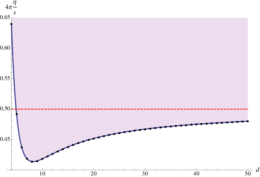
By combining eqs. (56) and (104), one obtains bounds on the ratio of the the shear viscosity to entropy density in the CFT’s dual to GB gravity. In particular, there is a lower bound which depends on the dimension of the bulk spacetime as:

\frac{\eta}{s}\geq\frac{1}{4\pi}\left[1-\frac{\left(D-1\right)\left(D-4\right)\left(D^{2}-3D+8\right)}{2\left(D^{2}-5D+10\right)^{2}}\right]\,.

(120)

For $D=5$ , we recover the result $\eta/s\geq 16/25\times(1/4\pi)=(0.640)/(4\pi)$ originally found in [15]. Recently, it was observed [17] that this function (120) has a minimum in the vicinity of $D=9$ , as illustrated in figure 9. More precisely, one finds a minimum value of $\eta/s\simeq(0.414)/(4\pi)$ for $D\simeq 9.207$ . Further for large $D$ , this lower bound rises again and asymptotically approaches $\eta/s=1/(8\pi)$ . It seems that these results may provide interesting empirical data in considering the question of a fundamental lower bound for $\eta/s$ , as was conjectured by [7]. However, it is not clear to us what conclusions one may draw with respect to this question at this point.

Within this class of CFT’s dual to GB gravity, one also finds an upper bound for the ratio of the shear viscosity to entropy density

\frac{\eta}{s}\leq\frac{1}{4\pi}\left[1+\frac{(D-1)(3D-1)}{2(D+1)^{2}}\right]\,.

(121)

As shown in figure 9, this upper bound is a monotonically increasing function which approaches $\eta/s=5/(8\pi)$ asymptotically for large $D$ . Of course, there is no fundamental interpretation of this upper bound since $\eta/s$ can become arbitrarily large for weakly coupled theories. Again, this bound only applies for the strongly coupled CFT’s with a holographic description in terms of GB gravity.

As also shown in figure 9, the previous upper bound is probably slightly lower in $d=4$ and 5 when one takes into account the plasma instabilities discussed in section 5.4. These instabilities do not indicate a fundamental pathology for the GB theories in the ranges given in eq. (83). Rather in these cases, one simply concludes that a homogenous plasma is an unstable configuration in the dual CFT. Since the unstable modes have large momentum, it seems that the plasma wants to “clump” into an inhomogeneous configuration. The immediate implication for our analysis is that the hydrodynamic calculations, and in particular, the computation of $\eta/s$ , is unreliable in this regime given in eq. (83). From a gravitational perspective, the plasma instabilities correspond to unstable quasinormal modes of the black hole background. It would be interesting to carry out a more extensive analysis of the quasinormal mode spectrum in GB gravity. This would likely provide greater insight into the nature of these instabilities.

Acknowledgments.

JE thanks Pedro Vieira for useful conversations. RCM would also like to thank Dam Son, Subir Sachdev and Andrei Starinets for useful conversations and correspondence. Research at Perimeter Institute is supported by the Government of Canada through Industry Canada and by the Province of Ontario through the Ministry of Research & Innovation. AB gratefully acknowledges further support by an NSERC Discovery grant and support through the Early Researcher Award program by the Province of Ontario. RCM also acknowledges support from an NSERC Discovery grant and funding from the Canadian Institute for Advanced Research. MFP is supported by the Portuguese Fundacao para a Ciencia e Tecnologia, grant SFRH/BD/23438/2005. MFP and MS would also like to thank the Perimeter Institute for hospitality at various stages of this project.

Appendix A Energy fluxes in terms of the three-point couplings

In this appendix we present an explicit computation of the energy flux (14) for a CFT in an arbitrary number of dimensions. In particular, $t_{2}$ and $t_{4}$ are determined in terms of the coefficients which appear in the three–point function of the stress–energy tensor [27, 26]. Our calculations closely follow those given in [17].

Let us consider the expression in eq. (24). Without loss of generality we can position the detector on the (positive) $x^{1}$ axis, i.e., $n^{i}=\delta^{i}{}_{1}$ as in section 3.3. We then introduce the light-cone coordinates $x^{\pm}=t\pm x^{1}$ and express the energy flux measured at large distances as

{\cal E}=\lim_{x^{+}\rightarrow\infty}\left({x^{+}-x^{-}\over 2}\right)^{d-2}\int dx^{-}\,T_{--}(x^{+},x^{-})

(122)

In order to determine $t_{2}$ and $t_{4}$ , it suffices to compute the energy one-point function (24) with specific polarizations which yield two independent linear combinations of these coefficients. Recalling the discussion at the beginning of section 3.3, we will consider polarizations in the tensor and vector channels. For the tensor channel, we choose a polarization where the only nonvanishing components are $\epsilon_{{\hat{\imath}}{\hat{\jmath}}}=\epsilon_{{\hat{\jmath}}{\hat{\imath}}}$ where ${\hat{\imath}}$ and ${\hat{\jmath}}$ are fixed indices with ${\hat{\imath}},{\hat{\jmath}}>1$ and ${\hat{\imath}}\neq{\hat{\jmath}}$ . Similarly for the vector channel, our polarization will only have nonvanishing components $\epsilon_{1{\hat{\imath}}}=\epsilon_{{\hat{\imath}}1}$ where ${\hat{\imath}}$ is again a fixed index with ${\hat{\imath}}>1$ . The corresponding linear combinations of $t_{2},t_{4}$ which will appear in eq. (14) are those appearing in the constraints (40) and (41). That is,

	$\displaystyle{\rm Tensor:}$		$\displaystyle\langle\mathcal{E}({\vec{n}})\rangle=\frac{E}{\Omega_{d-2}}\left[1-{1\over d-1}t_{2}-{2\over d^{2}-1}t_{4}\right]\,,$		(123)
	$\displaystyle{\rm Vector:}$		$\displaystyle\langle\mathcal{E}({\vec{n}})\rangle=\frac{E}{\Omega_{d-2}}\left[1+{d-3\over 2(d-1)}t_{2}-{2\over d^{2}-1}t_{4}\right]\,.$		(124)

We will present the details of the calculations for the tensor channel below. The vector channel calculations are a straightforward extension of these.

So choosing the tensor polarization above, the numerator of eq. (24) is proportional to the following three-point function

f_{3}(E)\equiv\int d^{\,d}x~e^{iEt}\lim_{x_{1}^{+}\rightarrow\infty}\left({x_{1}^{+}-x_{1}^{-}\over 2}\right)^{d-2}\int dx_{1}^{-}\ \langle\,T_{{\hat{\imath}}{\hat{\jmath}}}(x)\,T_{--}(x_{1}\,)\,T_{{\hat{\imath}}{\hat{\jmath}}}(0)\,\rangle

(125)

(where again ${\hat{\imath}}$ and ${\hat{\jmath}}$ are fixed indices and so no sum is intended above). Similarly, the normalisation in the denominator is provided by the two-point function

f_{2}(E)\equiv\int d^{\,d}x~e^{iEt}\,\langle\,T_{{\hat{\imath}}{\hat{\jmath}}}(x)\,T_{{\hat{\imath}}{\hat{\jmath}}}(0)\,\rangle\,.

(126)

In what follows we find it convenient to assume that the total number of space-time dimensions is even. In particular, this assumption allows to use the residue theorem in the evaluation of certain integrals. Since our final result turns out to be insensitive to the parity of the spacetime dimension, we analytically continue it (and implicitly the intermediate integrals) to any $d$ . Let us proceed with the evaluation of the numerator (125) and the denominator (126) separately.

We start with the denominator (126) where we can simply use the general result for two-point function (9). Inserting the indices ${\hat{\imath}}{\hat{\jmath}}$ and explicitly evaluating the general expression yields

\langle T_{{\hat{\imath}}{\hat{\jmath}}}(x)T_{{\hat{\imath}}{\hat{\jmath}}}(0)\rangle={C_{T}\over 2\left(x^{2}\right)^{d}}\left[1-{2\over x^{2}}\left((x^{\hat{\imath}})^{2}+(x^{\hat{\jmath}})^{2}\right)+{8\over\left(x^{2}\right)^{2}}(x^{\hat{\imath}})^{2}(x^{\hat{\jmath}})^{2}\right]~.

(127)

The central charge $C_{T}$ is given in eq. (13), which we present here again

C_{T}={\pi^{{d\over 2}}\over\Gamma\left({d/2}\right)}{(d-1)(d+2)\mathcal{A}-2\mathcal{B}-4(d+1)\mathcal{C}\over d(d+2)}\,.

(128)

The constants $\mathcal{A},\mathcal{B},\mathcal{C}$ are the parameters which control the three-point function of the stress tensor [27, 26]. To evaluate the integral in eq. (126), we must first provide an $i\epsilon$ prescription for the operators. Recall that the operators $T_{{\hat{\imath}}{\hat{\jmath}}}$ in this expression are not time-ordered which then requires that $t\rightarrow t-i\epsilon$ and so the light-cone coordinates are both replaced by $x^{\pm}\rightarrow x^{\pm}-i\epsilon$ . The various integrations are then best performed by first integrating over spatial directions which are perpendicular to $x^{1}$ , $x^{\hat{\imath}}$ and $x^{\hat{\jmath}}$ using $(d-4)$ -dimensional spherical polar coordinates, subsequently integrating over ( $x^{\hat{\imath}}$ , $x^{\hat{\jmath}}$ )-plane using polar coordinates and finally the $x^{\pm}$ integrals are performed using the residue theorem for the poles in these expressions. The latter integrals are

\int{dx^{+}\over\left(x^{+}-i\epsilon\right)^{{d\over 2}+1}}e^{i\frac{E}{2}x^{+}}\int{dx^{-}\over\left(x^{-}-i\epsilon\right)^{{d\over 2}+1}}e^{i\frac{E}{2}x^{-}}={(2\pi i)^{2}\over\Gamma\left({d+2\over 2}\right)^{2}}\,\left(iE\over 2\right)^{d}~.

(129)

This is the essential point where we assume that the dimension $d$ is even. Otherwise the singularities appearing in these integrals become branch cuts and the residue theorem can not be applied. Hence, our final result is given by

f_{2}(E)={\pi^{d+2\over 2}\over(d+1)}~{C_{T}\over\Gamma(d-1)\Gamma\left({d+2\over 2}\right)}\,\left({E\over 2}\right)^{d}\,.

(130)

Next we turn to computing eq. (125). Again we rely on the results of [27, 26] where the form of the three-point function of the stress tensor was completely fixed using conformal invariance and energy conservation – in particular, see (3.15) in [27].¹¹¹¹ 11 However, we express our results in terms of the parameters $\mathcal{A},\mathcal{B},\mathcal{C}$ of [26]. The corresponding parameters in [27] are given by: $a=\mathcal{A}/8$ , $b=(\mathcal{B}-2\mathcal{A})/8$ and $c=\mathcal{C}/2$ . Inserting the appropriate indices and taking the limit $x_{1}^{+}\rightarrow\infty$ , we find

\lim_{x_{1}^{+}\rightarrow\infty}\left({x_{1}^{+}-x_{1}^{-}\over 2}\right)^{d-2}\langle\,T_{{\hat{\imath}}{\hat{\jmath}}}(x)\,T_{--}(x_{1})\,T_{{\hat{\imath}}{\hat{\jmath}}}(0)\,\rangle={(-1)^{1-{3\over 2}\,d}\,2^{-(d+3)}\,(x^{-})^{2}\ t(x)\over\left(x^{-}_{1}-x^{-}+i\epsilon\right)^{d+2\over 2}\left(x^{-}_{1}-i\epsilon\right)^{d+2\over 2}\left(x^{2}\right)^{d+6\over 2}}

(131)

where

t(x)=-4\mathcal{B}\left[8(x^{\hat{\imath}})^{2}(x^{\hat{\jmath}})^{2}-x^{2}((x^{\hat{\imath}})^{2}+(x^{\hat{\jmath}})^{2})\right]+4\mathcal{C}\left[16(x^{\hat{\imath}})^{2}(x^{\hat{\jmath}})^{2}-2((x^{\hat{\imath}})^{2}+(x^{\hat{\jmath}})^{2})x^{2}+(x^{2})^{2}\right]\\ +\left[(d+2)(d-2)\mathcal{A}+(d-2)\mathcal{B}-4d\,\mathcal{C}\right]\left[x^{2}((x^{\hat{\imath}})^{2}+(x^{\hat{\jmath}})^{2})-8(x^{\hat{\imath}})^{2}(x^{\hat{\jmath}})^{2}\right]\\ +8(d+2)\left((d-2)\,\mathcal{A}+\mathcal{B}-4\mathcal{C}\right)(x^{\hat{\imath}})^{2}(x^{\hat{\jmath}})^{2}+2(d+4)(d-2)(\mathcal{B}-2\mathcal{C})(x^{\hat{\imath}})^{2}(x^{\hat{\jmath}})^{2}~.

(132)

In the expression above, the $i\epsilon$ prescription was $t_{1}\to t_{1}-i\epsilon$ and $t\to t-2i\epsilon$ , giving a larger negative imaginary part to time in operators standing to the left. Integrating over $x_{1}^{-}$ includes only one of the poles in eq. (131), irrespective of whether the contour is closed in the upper or lower half of the $x_{1}^{-}$ -plane. In either case, the integral yields

\int dx_{1}^{-}\lim_{x_{1}^{+}\rightarrow\infty}\left({x_{1}^{+}-x_{1}^{-}\over 2}\right)^{d-2}\langle\,T_{{\hat{\imath}}{\hat{\jmath}}}(x)\,T_{--}(x_{1})\,T_{{\hat{\imath}}{\hat{\jmath}}}(0)\,\rangle\\ =2\pi i~{\Gamma(d+1)\over\Gamma\left({d+2\over 2}\right)^{2}}{2^{-(d+3)}\,t(x)\over\left(x^{-}-2i\epsilon\right)^{d-1}\left(x^{2}\right)^{d+6\over 2}}~.

(133)

Performing the remaining integrals over $x^{a}$ in eq. (125) as described in the previous case, the final result becomes

f_{3}(E)=-\frac{E}{8}\left({E\over 4}\right)^{d}{2\pi^{d+4\over 2}\over\Gamma\left({d+4\over 2}\right)\Gamma\left({d+2\over 2}\right)^{2}}\,\left((d-2)\,(d+2)\,\mathcal{A}+2\,d\,\mathcal{B}-4\,d\,\mathcal{C}\right)\,.

(134)

Note that in this case, the integrals over the light-cone coordinates are

\int{dx^{+}\over\left(x^{+}-2i\epsilon\right)^{2}}e^{i\frac{E}{2}x^{+}}\int{dx^{-}\over\left(x^{-}-2i\epsilon\right)^{d+1}}e^{i\frac{E}{2}x^{-}}={\left(2\pi i\right)^{2}}{1\over\Gamma(d+1)}\left({iE\over 2}\right)^{d+1}~,

(135)

and so yield poles irrespective of whether $d$ is even or odd.

Combining the expressions in eqs. (130) and (134) then yields

{\Omega_{d-2}\over E}~{f_{3}(E)\over f_{2}(E)}=-{d+1\over d}~{(d-2)\,(d+2)\,\mathcal{A}+2\,d\,\mathcal{B}-4\,d\,\mathcal{C}\over(d-1)(d+2)\,\mathcal{A}-2\,\mathcal{B}-4(d+1)\,\mathcal{C}}~.

(136)

Note that producing this expression requires the use of an identity for $\Gamma$ functions of the form:

\Gamma\!\left(\frac{d}{2}\right)\ \Gamma\!\left(\frac{d-1}{2}\right)=\sqrt{\pi}\ 2^{2-d}\ \Gamma\left(d-1\right)\,.

(137)

Comparing the previous expression with eq. (123), we find our first linear combination of $t_{2}$ and $t_{4}$ :

1-{1\over d-1}t_{2}-{2\over d^{2}-1}t_{4}=-{d+1\over d}~{(d-2)\,(d+2)\,\mathcal{A}+2\,d\,\mathcal{B}-4\,d\,\mathcal{C}\over(d-1)(d+2)\,\mathcal{A}-2\,\mathcal{B}-4(d+1)\,\mathcal{C}}~.

(138)

Following the same basic steps as above, one can also compute the flux with the vector channel polarization to produce the linear combination of $t_{2}$ and $t_{4}$ in eq. (124). The computations are somewhat more involved in this case and we only present the final result:

1+{d-3\over 2(d-1)}t_{2}-{2\over d^{2}-1}t_{4}=(d+1)~{(d-2)\,(d+2)\,\mathcal{A}+(3d-2)\,\mathcal{B}-8\,d\,\mathcal{C}\over(d-1)(d+2)\,\mathcal{A}-2\,\mathcal{B}-4(d+1)\,\mathcal{C}}~.

(139)

Combining eqs. (138) and (139), we can solve for $t_{2}$ and $t_{4}$ separately,

	$\displaystyle t_{2}$	$\displaystyle=$	$\displaystyle\frac{2(d+1)}{d}\,{(d-2)\,(d+2)\,(d+1)\,\mathcal{A}+3\,d^{\,2}\,\mathcal{B}-4\,d\,(2d+1)\,\mathcal{C}\over(d-1)(d+2)\,\mathcal{A}-2\,\mathcal{B}-4(d+1)\,\mathcal{C}}~,$		(140)
	$\displaystyle t_{4}$	$\displaystyle=$	$\displaystyle-{(d+1)\over d}~{~(d+2)\,(2d^{2}-3d-3)\,\mathcal{A}+2\,d^{\,2}\,(d+2)\,\mathcal{B}-4d\,(d+1)\,(d+2)\,\mathcal{C}\over(d-1)(d+2)\,\mathcal{A}-2\,\mathcal{B}-4(d+1)\,\mathcal{C}}~.$

Note that these expressions for general $d$ reproduce the results presented in [18] and [17] in $d=4,6$ respectively.

Appendix B Conformal tensor fields

In sections 3.3 and 7, we compare various results for the strongly coupled CFT’s dual to GB gravity to those for massless free fields. As well as conformally coupled scalars and massless fermions, an ( $n$ –1)-form potential in $d=2n$ dimensions yields another free field theory which is also conformally invariant. The most familiar example is provided by $d=4$ , in which case the potential is just an Abelian vector field. Our final results given in eq. (155) are general expressions for $\mathcal{A}$ , $\mathcal{B}$ and $\mathcal{C}$ for any value of $n$ . The analysis leading to these expression is quite involved and we only provide some of the salient steps in the following. Further, for simplicity, we work in a Euclidean-signature space.

We begin with a free $(n-1)$ –form gauge field $A$ in $d=2n$ dimensions. As usual, the corresponding field strength is an $n$ -form given by $F=dA$ . With a general background metric, the action for this system is

I={1\over 2(n!)}\int d^{\,2n}x\sqrt{g}g^{\mu_{1}\nu_{1}}g^{\mu_{2}\nu_{2}}\cdots g^{\mu_{n}\nu_{n}}\,F_{\mu_{1}\mu_{2}\cdots\mu_{n}}\,F_{\nu_{1}\nu_{2}\cdots\nu_{n}}\,,

(141)

which is invariant under conformal rescalings, $g_{\mu\nu}\to e^{2\phi}g_{\mu\nu}$ . To simplify the subsequent calculations, we now fix the background metric to be simply flat space, i.e., $g_{\mu\nu}=\delta_{\mu\nu}$ . The corresponding energy momentum tensor is given by

T_{\mu\nu}={1\over(n-1)!}F_{\mu\,\alpha_{2}\cdot\cdot\cdot\alpha_{n}}F_{\nu}^{~\alpha_{2}\cdot\cdot\cdot\alpha_{n}}-{1\over 2(n!)}\delta_{\mu\nu}\,F_{\alpha_{1}\cdot\cdot\cdot\alpha_{n}}F^{\alpha_{1}\cdot\cdot\cdot\alpha_{n}}\quad.

(142)

Because the theory is invariant under gauge transformations $\delta A=d\Lambda$ , in principle, we should introduce gauge-fixing terms to the action (141). However, correlation functions involving only gauge invariant operators will be unaffected by the choice of gauge-fixing and any ghost fields and so we do not consider the complete details here. With the natural generalization of Feynman gauge, the two-point function of the potential becomes

\langle\,A_{\mu_{1}\cdot\cdot\cdot\mu_{n-1}}(x_{1})A_{\nu_{1}\cdot\cdot\cdot\nu_{n-1}}(x_{2})\,\rangle={\Gamma(n-1)\over 4\,\pi^{n}}{1\over(x_{12}^{2})^{n-1}}\sum_{\sigma\in S_{n-1}}\mathrm{sign}(\sigma)\,\delta_{\mu_{1}\nu_{\sigma(1)}}\cdot\cdot\cdot\delta_{\mu_{n-1}\nu_{\sigma(n-1)}}

(143)

where $S_{n-1}$ is a permutation group of $n-1$ elements $1,2,..,n-1$ . Differentiating the above two-point function with respect to $x_{1}^{\mu_{n}}$ and $x_{2}^{\nu_{n}}$ and subsequently antisymmetrizing the result with respect to $\mu$ ’s and $\nu$ ’s yields the following basic gauge invariant two-point function of the field strength

\langle\,F_{\mu_{1}\cdot\cdot\cdot\mu_{n}}(x)F_{\nu_{1}\cdot\cdot\cdot\nu_{n}}(0)\,\rangle={n\over\Omega_{2n-1}}~{J_{\mu_{1}\cdot\cdot\cdot\mu_{n}\,;\,\nu_{1}\cdot\cdot\cdot\nu_{n}}\over(x^{2})^{n}}\quad,

(144)

where

J_{\mu_{1}\cdot\cdot\cdot\mu_{n}\,;\,\nu_{1}\cdot\cdot\cdot\nu_{n}}(x)=\sum_{\sigma\in S_{n}}\mathrm{sign}(\sigma)\,I_{\mu_{1}\nu_{\sigma(1)}}(x)\cdot\cdot\cdot I_{\mu_{n}\nu_{\sigma(n)}}(x)\quad.

(145)

As in eq. (11), we have defined the orthogonal matrix

I_{\mu\nu}(x)=\delta_{\mu\nu}-2\frac{x_{\mu}\,x_{\nu}}{x^{2}}\,.

(146)

After a lengthy calculation, we arrive at the connected two-point function of the energy momentum tensor

\langle T_{\mu\nu}(x)\,T_{\alpha\beta}(0)\rangle={n^{2}\,\Gamma[2n-1]\over 2\pi^{2n}}\,{1\over(x^{2})^{2n}}\,\mathcal{I}_{\mu\nu,\alpha\beta}(x)~,

(147)

where $\mathcal{I}_{\mu\nu,\alpha\beta}(x)$ is defined as in eq. (10). Of course, our result matches the expected form given in eq. (9) where

C_{\,T}={d^{\,2}\over 8\,\pi^{\,d}}\,\Gamma[d-1]\quad.

(148)

Proceeding further requires calculating the three-point function of the stress tensor. While such a computation is straightforward, it would be extremely tedious to carry out in general. The calculations are greatly simplified by going to the collinear frame [27], for which the three points are chosen to lie on a straight line. In this case, the form of the three-point function is given by eqs. (4.20) and (4.21) of [27]. Since we wish to fix the values of $\mathcal{A}$ , $\mathcal{B}$ and $\mathcal{C}$ , it is enough to supplement eq. (148) with two extra relations between these constants. We choose to compute coefficients $\alpha$ and $\gamma$ defined in eq. (4.21) of [27].

For simplicity, we exploit the rotational and translational symmetry of the problem to choose the following three points for the insertions of the energy momentum tensor: $x_{1}=(x,\mathbf{0})$ , $x_{2}=(y,\mathbf{0})$ , $x_{3}=0$ . As a result, $I_{\mu\nu}$ becomes a constant orthogonal matrix given by

I_{\mu\nu}=\delta_{\mu\nu}-2\,\delta_{1\mu}\delta_{1\nu}~.

(149)

With some work, we find

\langle T_{11}(x)T_{11}(y)T_{11}(0)\rangle=-{n^{2}\,\Gamma(n)\Gamma(2n)\over 4\,\pi^{3n}}{1\over x^{2n}y^{2n}(x-y)^{2n}}\quad,

(150)

and hence, in the notation of [27],

\alpha=-{d^{2}\,\Gamma(d/2)\Gamma(d)\over 16\,\pi^{3d/2}}\quad.

(151)

Similarly, we obtain

\langle T_{i1}(x)T_{j1}(y)T_{11}(0)\rangle=\,{n^{3}\,\Gamma(n)\,\Gamma(2n-1)\over 4\pi^{3n}}{\delta_{ij}\over x^{2n}y^{2n}(x-y)^{2n}}\quad,

(152)

which yields

\gamma=\,{d^{3}\,\Gamma(d/2)\,\Gamma(d-1)\over 32\,\pi^{\,3d/2}}\quad.

(153)

According to eqs. (4.22 $\,-\,$ 4.25) of [27],

	$\displaystyle\alpha$	$\displaystyle=$	$\displaystyle-{(d-1)(d^{\,3}-2\,d^{\,2}-d+4)\over 2\,d^{\,2}}\,\mathcal{A}+{(d-1)^{3}\over 4\,d}\,\mathcal{B}-{(d+1)(d-1)^{2}(d-4)\over 2\,d^{\,2}}\,\mathcal{C}~,$
	$\displaystyle\gamma$	$\displaystyle=$	$\displaystyle{d^{\,3}-\,d^{\,2}-2\,d+4\over 8\,d}\,\mathcal{A}+{(d-3)\over 8}\,\mathcal{B}-{(d+1)(d-1)\over 2\,d}\,\mathcal{C}~.$		(154)

Hence combining these two equations with (13),(148),(151),(153) and solving for $\mathcal{A}$ , $\mathcal{B}$ and $\mathcal{C}$ yields

$\displaystyle\mathcal{A}$	$\displaystyle=$	$\displaystyle-{d^{3}\Gamma(d-1)\Gamma(d/2)\over 8(d-3)\pi^{3d/2}}~,$
$\displaystyle\mathcal{B}$	$\displaystyle=$	$\displaystyle(d-2)\,\mathcal{A}~,$	(155)
$\displaystyle\mathcal{C}$	$\displaystyle=$	$\displaystyle{d-2\over 2}\,\mathcal{A}~.$

These general results agree with those derived for $d=4$ in [27] and for $d=6$ in [17].

Appendix C Useful expressions

In order to write our equations as neatly as possible, we define the following expressions, which appear repeatedly in our analysis:

\mathcal{K}=u^{\frac{D-1}{2}}=1-f+\lambda_{\text{\tiny{GB}}}f^{2},

\mathcal{M}=1-2\frac{(D-1)}{(D-3)}\lambda_{\text{\tiny{GB}}}-2\frac{(D-5)}{(D-3)}\lambda_{\text{\tiny{GB}}}f\left(1-\lambda_{\text{\tiny{GB}}}f\right),

\mathcal{N}=\left[1-2\lambda_{\text{\tiny{GB}}}f\right]^{2},

	$\displaystyle\mathcal{P}=$	$\displaystyle-\frac{1}{2}(D-1)\left[1-\frac{2(D-1)}{(D-3)}\lambda_{\text{\tiny{GB}}}\right]+\left[1+\frac{2(D-1)(D-6)}{(D-3)}\lambda_{\text{\tiny{GB}}}\right]f-$
		$\displaystyle+\frac{1}{2(D-3)(D-4)}\left[172-91D+16D^{2}-D^{3}+8(D-1)(D-4)(2D-9)\lambda_{\text{\tiny{GB}}}\right]\lambda_{\text{\tiny{GB}}}f^{2}+$
		$\displaystyle+\frac{2}{(D-3)^{2}}\left[87-44D+5D^{2}+4(D-1)(D-3)(D-4)\lambda_{\text{\tiny{GB}}}\right]\lambda_{\text{\tiny{GB}}}^{2}f^{3}-$
		$\displaystyle+\frac{(D-5)(D+15)}{(D-3)}\lambda_{\text{\tiny{GB}}}^{3}f^{4}+\frac{8(D-5)}{(D-3)}\lambda_{\text{\tiny{GB}}}^{4}f^{5},$

	$\displaystyle\mathcal{R}=\frac{(D-1)^{2}}{64f_{\infty}}\Biggl[$	$\displaystyle 4f_{\infty}{\swabfamily w}^{2}\left[1-\frac{2(D-1)}{(D-3)}\lambda_{\text{\tiny{GB}}}\right]$
		$\displaystyle+4\biggl[{\swabfamily q}^{2}\left[\frac{2(D-1)}{(D-3)(D-4)}\lambda_{\text{\tiny{GB}}}\left[2(D-1)\lambda_{\text{\tiny{GB}}}+D-6\right]-1\right]+$
		$\displaystyle+\frac{2f_{\infty}{\swabfamily w}^{2}}{(D-3)}\lambda_{\text{\tiny{GB}}}\left[4(D-1)\lambda_{\text{\tiny{GB}}}-3D+11\right]\biggr]f-$
		$\displaystyle+\frac{4}{(D-3)(D-4)}\biggl[2{\swabfamily q}^{2}\left[4(D-1)(2D-7)\lambda_{\text{\tiny{GB}}}-3D(D-7)-42\right]+$
		$\displaystyle+2(D-4)f_{\infty}{\swabfamily w}^{2}\lambda_{\text{\tiny{GB}}}\left[4(D-1)\lambda_{\text{\tiny{GB}}}-7D+31\right]\biggr]\lambda_{\text{\tiny{GB}}}f^{2}+$
		$\displaystyle+\frac{8}{(D-3)(D-4)}\biggl[4\lambda_{\text{\tiny{GB}}}\left[{\swabfamily q}^{2}(D-1)(2D-7)-2(D-4)(D-5)f_{\infty}{\swabfamily w}^{2}\right]-$
		$\displaystyle+{\swabfamily q}^{2}\left[5D(D-9)+112\right]\biggr]\lambda_{\text{\tiny{GB}}}^{2}f^{3}+\frac{16(D-5)}{(D-3)(D-4)}\bigl[2{\swabfamily q}^{2}(D-7)+$
		$\displaystyle+2(D-4)f_{\infty}{\swabfamily w}^{2}\lambda_{\text{\tiny{GB}}}\bigr]\lambda_{\text{\tiny{GB}}}^{3}f^{4}-\frac{16(D-5)(D-7){\swabfamily q}^{2}}{(D-3)(D-4)}\lambda_{\text{\tiny{GB}}}^{4}f^{5}\Biggr],$

\mathcal{S}=-\frac{3}{4}(D-1)+\frac{1}{4}\left[3+D+10(D-1)\lambda_{\text{\tiny{GB}}}\right]f-\frac{1}{4}(5D+11)\lambda_{\text{\tiny{GB}}}f^{2}+\frac{1}{2}(D+7)\lambda_{\text{\tiny{GB}}}^{2}f^{3},

\mathcal{T}=-\frac{(D-1)}{4}+\frac{1}{4}\left[5-D+6(D-1)\lambda_{\text{\tiny{GB}}}\right]f+\frac{1}{4}(D-17)\lambda_{\text{\tiny{GB}}}f^{2}-\frac{1}{2}(D-9)\lambda_{\text{\tiny{GB}}}^{2}f^{3},

\mathcal{V}=\frac{1}{2(D-2)}\biggl[(D-1)+\left[D-3-6(D-1)\lambda_{\text{\tiny{GB}}}\right]f-(D-9)\lambda_{\text{\tiny{GB}}}f^{2}+2(D-5)\lambda_{\text{\tiny{GB}}}^{2}f^{3}\biggr].

Appendix D Coefficients for the sound channel

	Numerator of	$\displaystyle\mathcal{C}^{(1)}_{\text{\tiny{sound}}}=\,2(D-3){\swabfamily q}^{2}f^{2}\mathcal{M}\biggl[2(D-1)(D-2)\lambda_{\text{\tiny{GB}}}f_{\infty}{\swabfamily w}^{2}\mathcal{M}\mathcal{N}\mathcal{K}+{\swabfamily q}^{2}\mathcal{N}\mathcal{P}+$
		$\displaystyle-(D-3){\swabfamily q}^{2}\mathcal{M}^{2}\mathcal{T}+\mathcal{M}\Bigl[(D-3)\left({\swabfamily q}^{2}\mathcal{P}-(D-2)f_{\infty}{\swabfamily w}^{2}\mathcal{N}^{2}\right)-{\swabfamily q}^{2}\mathcal{N}\mathcal{T}\Bigr]\biggr]+$
		$\displaystyle-(D-2)\mathcal{N}^{1/2}\mathcal{P}\Bigl[(D-1){\swabfamily q}^{2}\mathcal{K}-2(D-2)f_{\infty}{\swabfamily w}^{2}\mathcal{N}^{1/2}\Bigr]\Bigl[{\swabfamily q}^{2}\mathcal{V}-f_{\infty}{\swabfamily w}^{2}\mathcal{N}\Bigr]+$
		$\displaystyle-{\swabfamily q}^{2}f\Biggl[-2(D-1)^{2}(D-2)\lambda_{\text{\tiny{GB}}}\mathcal{M}\mathcal{N}^{1/2}\mathcal{K}^{2}\left(f_{\infty}{\swabfamily w}^{2}\mathcal{N}-{\swabfamily q}^{2}\mathcal{V}\right)+$
		$\displaystyle+(D-1)(D-3)\mathcal{M}\mathcal{N}^{1/2}\mathcal{K}\Bigl[(D-2)f_{\infty}{\swabfamily w}^{2}\mathcal{N}^{2}+{\swabfamily q}^{2}\left(\mathcal{M}\mathcal{T}-\mathcal{P}\right)+$
		$\displaystyle+(D-2){\swabfamily q}^{2}\left(2\mathcal{M}-\mathcal{N}\right)\mathcal{V}\Bigr]+2(D-2)\Bigl[f_{\infty}{\swabfamily w}^{2}\left((D-3)\mathcal{M}-\mathcal{N}\right)\mathcal{N}\mathcal{P}+$
		$\displaystyle+{\swabfamily q}^{2}\bigl[\mathcal{N}\mathcal{P}+(D-3)\mathcal{M}^{2}\mathcal{S}\bigr]\mathcal{V}\Bigr]\Biggr],$

	$\displaystyle\text{Denominator of }\mathcal{C}^{(1)}_{\text{\tiny{sound}}}=$	$\displaystyle\,(D-2)uf\mathcal{M}\mathcal{N}\left(f_{\infty}{\swabfamily w}^{2}\mathcal{N}-{\swabfamily q}^{2}\mathcal{V}\right)\biggl[2{\swabfamily q}^{2}f\left((D-3)\mathcal{M}+\mathcal{N}\right)+$
		$\displaystyle(D-1){\swabfamily q}^{2}\mathcal{N}^{1/2}\mathcal{K}-2(D-2)f_{\infty}{\swabfamily w}^{2}\mathcal{N}\biggr],$

Numerator of $\mathcal{C}^{(2)}_{\text{\tiny{sound}}}$ =

		$\displaystyle(D-1)\Biggl[\mathcal{N}^{1/2}\left[(D-1){\swabfamily q}^{2}\mathcal{K}-2(D-2)f_{\infty}{\swabfamily w}^{2}\mathcal{N}^{1/2}\right]\biggl[{\swabfamily q}^{2}\mathcal{K}\Bigl[-(D-1)^{2}u\mathcal{N}\Bigl[-2{\swabfamily q}^{2}\mathcal{P}+$
		$\displaystyle+\mathcal{M}\left(5(D-2)f_{\infty}{\swabfamily w}^{2}\mathcal{N}+2{\swabfamily q}^{2}\mathcal{T}\right)\Bigr]+(D-2)\left[\mathcal{M}\left((D-1)^{2}{\swabfamily q}^{2}u\mathcal{N}-8(D-2)f_{\infty}\mathcal{S}\right)-8(D-2)f_{\infty}\mathcal{P}\right]\mathcal{V}\Bigr]+$
		$\displaystyle+4(D-1)(D-2)f_{\infty}{\swabfamily q}^{2}\mathcal{N}^{1/2}\mathcal{K}^{2}\left[\mathcal{P}-\mathcal{M}\left(\mathcal{T}+2(D-2)\mathcal{V}\right)\right]+2(D-1)(D-2)f_{\infty}u{\swabfamily w}^{2}\mathcal{N}^{3/2}\times$
		$\displaystyle\left[-2{\swabfamily q}^{2}\mathcal{P}+\mathcal{M}\left[(D-2)f_{\infty}{\swabfamily w}^{2}\mathcal{N}-{\swabfamily q}^{2}\left(2\mathcal{S}+(D-2)\mathcal{V}\right)\right]\right]\biggr]+4{\swabfamily q}^{2}f^{2}\biggl[8(D-1)(D-2)^{2}f_{\infty}\lambda_{\text{\tiny{GB}}}\mathcal{M}\mathcal{K}^{2}\times$
		$\displaystyle\Bigl[(D-3)f_{\infty}{\swabfamily w}^{2}\mathcal{M}\mathcal{N}+{\swabfamily q}^{2}\left((D-3)\mathcal{M}+\mathcal{N}\right)\mathcal{V}\Bigr]+(D-1){\swabfamily q}^{2}u\mathcal{N}^{1/2}\left((D-3)\mathcal{M}+\mathcal{N}\right)\times$
		$\displaystyle\Bigl[2{\swabfamily q}^{2}\mathcal{N}\mathcal{P}-(D-3)\mathcal{M}^{2}\left[(D-2)f_{\infty}{\swabfamily w}^{2}\mathcal{N}+{\swabfamily q}^{2}\left(2\mathcal{T}-(D-2)\mathcal{V}\right)\right]+\mathcal{M}\bigl[-(D-2)(2D-5)f_{\infty}{\swabfamily w}^{2}\mathcal{N}^{2}+$
		$\displaystyle+2(D-3){\swabfamily q}^{2}\mathcal{P}+{\swabfamily q}^{2}\mathcal{N}\left((D-2)\mathcal{V}-2\mathcal{T}\right)\bigr]\Bigr]+2(D-2)f_{\infty}\mathcal{K}\Bigl[2{\swabfamily q}^{2}\mathcal{N}^{2}\mathcal{P}-4(D-3)^{2}{\swabfamily q}^{2}\mathcal{M}^{3}\mathcal{T}+$
		$\displaystyle+{\swabfamily q}^{2}\mathcal{M}\mathcal{N}\bigl[2(D-1)^{2}\lambda_{\text{\tiny{GB}}}u{\swabfamily w}^{2}\mathcal{N}^{3/2}+6(D-3)\mathcal{P}-2\mathcal{N}\left(\mathcal{T}+(D-2)(D-3)\mathcal{V}\right)\bigr]+$
		$\displaystyle+(D-3)\mathcal{M}^{2}\Bigl[2(D-1)^{2}\lambda_{\text{\tiny{GB}}}{\swabfamily q}^{2}u{\swabfamily w}^{2}\mathcal{N}^{3/2}-2(D-2)(D-3)f_{\infty}{\swabfamily w}^{2}\mathcal{N}^{2}+4(D-3){\swabfamily q}^{2}\mathcal{P}+$
		$\displaystyle-2{\swabfamily q}^{2}\mathcal{N}\left(3\mathcal{T}+(D-2)(D-3)\mathcal{V}\right)\Bigr]\Bigr]\biggr]+4{\swabfamily q}^{2}f\biggl[4(D-1)^{2}(D-2)^{2}f_{\infty}^{2}\lambda_{\text{\tiny{GB}}}{\swabfamily w}^{2}\mathcal{M}\mathcal{N}^{3/2}\mathcal{K}^{3}+$
		$\displaystyle+2(D-1)(D-2)f_{\infty}u{\swabfamily w}^{2}\mathcal{N}^{3/2}\Bigl[-2{\swabfamily q}^{2}\mathcal{N}\mathcal{P}+(D-3)\mathcal{M}^{2}\left[(D-2)f_{\infty}{\swabfamily w}^{2}\mathcal{N}+{\swabfamily q}^{2}\left(\mathcal{T}-\mathcal{S}-(D-2)\mathcal{V}\right)\right]+$
		$\displaystyle+\mathcal{M}\bigl[(D-2)^{2}f_{\infty}{\swabfamily w}^{2}\mathcal{N}^{2}-2(D-3){\swabfamily q}^{2}\mathcal{P}+{\swabfamily q}^{2}\mathcal{N}\left(\mathcal{T}-\mathcal{S}-(D-2)\mathcal{V}\right)\bigr]\Bigr]+(D-1)(D-2)f_{\infty}\mathcal{N}^{1/2}\mathcal{K}^{2}\times$
		$\displaystyle\Bigl[4{\swabfamily q}^{2}\mathcal{N}\mathcal{P}-2(D-3){\swabfamily q}^{2}\mathcal{M}^{2}\left(3\mathcal{T}+4(D-2)\mathcal{V}\right)+\mathcal{M}\bigl[2(D-1)^{2}\lambda_{\text{\tiny{GB}}}{\swabfamily q}^{2}u{\swabfamily w}^{2}\mathcal{N}^{3/2}+$
		$\displaystyle-2(D-2)(D-3)f_{\infty}{\swabfamily w}^{2}\mathcal{N}^{2}+6(D-3){\swabfamily q}^{2}\mathcal{P}-8(D-2)^{2}f_{\infty}\lambda_{\text{\tiny{GB}}}{\swabfamily w}^{2}\mathcal{N}^{1/2}\mathcal{V}-4{\swabfamily q}^{2}\mathcal{N}\left(\mathcal{T}+(D-2)\mathcal{V}\right)\bigr]\Bigr]+$
		$\displaystyle+\mathcal{K}\Bigl[2\mathcal{N}\mathcal{P}\left[\left((D-1)^{2}{\swabfamily q}^{4}u-2(D-2)^{2}f_{\infty}^{2}{\swabfamily w}^{2}\right)\mathcal{N}-2(D-2)^{2}f_{\infty}{\swabfamily q}^{2}\mathcal{V}\right]+(D-3)\mathcal{M}^{2}\times$
		$\displaystyle\bigl[\mathcal{N}\bigl[-3(D-1)^{2}(D-2)f_{\infty}{\swabfamily q}^{2}u{\swabfamily w}^{2}\mathcal{N}-2\left((D-1)^{2}{\swabfamily q}^{4}u-2(D-2)^{2}f_{\infty}^{2}{\swabfamily w}^{2}\right)\mathcal{T}\bigr]+$
		$\displaystyle+(D-2){\swabfamily q}^{2}\left((D-1)^{2}{\swabfamily q}^{2}u\mathcal{N}-8(D-2)f_{\infty}\mathcal{S}\right)\mathcal{V}\bigr]+\mathcal{M}\mathcal{N}\bigl[-4(D-1)^{2}(D-2)^{2}f_{\infty}^{2}\lambda_{\text{\tiny{GB}}}u{\swabfamily w}^{4}\mathcal{N}^{3/2}+$
		$\displaystyle-D(D-1)^{2}(D-2)f_{\infty}{\swabfamily q}^{2}u{\swabfamily w}^{2}\mathcal{N}^{2}+2(D-3)\bigl((D-1)^{2}{\swabfamily q}^{4}u-6(D-2)^{2}f_{\infty}^{2}{\swabfamily w}^{2}\bigr)\mathcal{P}-4(D-2)^{2}f_{\infty}{\swabfamily q}^{2}\mathcal{S}\mathcal{V}+$
		$\displaystyle+\mathcal{N}\bigl[-2\mathcal{T}\left((D-1)^{2}{\swabfamily q}^{4}u-2(D-2)^{2}f_{\infty}^{2}{\swabfamily w}^{2}\right)+(D-2)\bigl((D-1)^{2}{\swabfamily q}^{4}u+4(D-2)^{2}(D-3)f_{\infty}^{2}{\swabfamily w}^{2}\bigr)\mathcal{V}\bigr]\bigr]\Bigr]\biggr]\Biggr],$

	$\displaystyle\text{Denominator of }\mathcal{C}^{(2)}_{\text{\tiny{sound}}}=\,$	$\displaystyle 32(D-2)^{2}f_{\infty}u^{2}f^{2}\mathcal{M}\mathcal{N}^{3/2}\left(f_{\infty}{\swabfamily w}^{2}\mathcal{N}-{\swabfamily q}^{2}\mathcal{V}\right)\biggl[2{\swabfamily q}^{2}f\left((D-3)\mathcal{M}+\mathcal{N}\right)$
		$\displaystyle+(D-1){\swabfamily q}^{2}\mathcal{N}^{1/2}\mathcal{K}-2(D-2)f_{\infty}{\swabfamily w}^{2}\mathcal{N}\biggr],$

References

[1] J. M. Maldacena, “The large N limit of superconformal field theories and supergravity,” Adv. Theor. Math. Phys. 2, 231 (1998) [Int. J. Theor. Phys. 38, 1113 (1999)] [arXiv:hep-th/9711200].
[2] E. Witten, “Anti-de Sitter space and holography,” Adv. Theor. Math. Phys. 2, 253 (1998) [arXiv:hep-th/9802150].
[3] S. S. Gubser, I. R. Klebanov and A. M. Polyakov, “Gauge theory correlators from non-critical string theory,” Phys. Lett. B 428, 105 (1998) [arXiv:hep-th/9802109].
[4] R. Baier, P. Romatschke, D. T. Son, A. O. Starinets and M. A. Stephanov, “Relativistic viscous hydrodynamics, conformal invariance, and holography,” JHEP 0804, 100 (2008) [arXiv:0712.2451 [hep-th]].
[5] S. Bhattacharyya, V. E. Hubeny, S. Minwalla and M. Rangamani, “Nonlinear Fluid Dynamics from Gravity,” JHEP 0802, 045 (2008) [arXiv:0712.2456 [hep-th]].
[6] D. T. Son and A. O. Starinets, “Viscosity, Black Holes, and Quantum Field Theory,” Ann. Rev. Nucl. Part. Sci. 57, 95 (2007) [arXiv:0704.0240 [hep-th]].
[7] P. Kovtun, D. T. Son and A. O. Starinets, “Viscosity in strongly interacting quantum field theories from black hole physics,” Phys. Rev. Lett. 94, 111601 (2005) [arXiv:hep-th/0405231].
[8] A. Buchel and J. T. Liu, “Universality of the shear viscosity in supergravity,” Phys. Rev. Lett. 93, 090602 (2004) [arXiv:hep-th/0311175];
A. Buchel, J. T. Liu and A. O. Starinets, “Coupling constant dependence of the shear viscosity in N=4 supersymmetric Yang-Mills theory,” Nucl. Phys. B 707, 56 (2005) [arXiv:hep-th/0406264];
A. Buchel, “On universality of stress-energy tensor correlation functions in supergravity,” Phys. Lett. B 609, 392 (2005) [arXiv:hep-th/0408095];
P. Benincasa, A. Buchel and R. Naryshkin, “The shear viscosity of gauge theory plasma with chemical potentials,” Phys. Lett. B 645, 309 (2007) [arXiv:hep-th/0610145];
D. Mateos, R. C. Myers and R. M. Thomson, “Holographic viscosity of fundamental matter,” Phys. Rev. Lett. 98, 101601 (2007) [arXiv:hep-th/0610184];
K. Landsteiner and J. Mas, “The shear viscosity of the non-commutative plasma,” JHEP 0707, 088 (2007) [arXiv:0706.0411 [hep-th]];
R. C. Myers, M. F. Paulos and A. Sinha, “Quantum corrections to $\eta/s$ ,” Phys. Rev. D 79, 041901 (2009) [arXiv:0806.2156 [hep-th]];
N. Iqbal and H. Liu, “Universality of the hydrodynamic limit in AdS/CFT and the membrane paradigm,” Phys. Rev. D 79, 025023 (2009) [arXiv:0809.3808 [hep-th]].
[9] E. Imeroni and A. Sinha, “Non-relativistic metrics with extremal limits,” JHEP 0909, 096 (2009) [arXiv:0907.1892 [hep-th]];
M. Edalati, J. I. Jottar and R. G. Leigh, “Transport Coefficients at Zero Temperature from Extremal Black Holes,” arXiv:0910.0645 [hep-th];
M. F. Paulos, “Transport coefficients, membrane couplings and universality at extremality,” arXiv:0910.4602 [hep-th];
S. K. Chakrabarti, S. Jain and S. Mukherji, “Viscosity to entropy ratio at extremality,” arXiv:0910.5132 [hep-th];
R. G. Cai, Y. Liu and Y. W. Sun, “Transport Coefficients from Extremal Gauss-Bonnet Black Holes,” arXiv:0910.4705 [hep-th].
[10] For example, see:
D. Teaney, “Effect of shear viscosity on spectra, elliptic flow, and Hanbury Brown-Twiss radii,” Phys. Rev. C 68 (2003) 034913 [arXiv:nucl-th/0301099];
A. Adare et al. [PHENIX Collaboration], “Energy Loss and Flow of Heavy Quarks in Au+Au Collisions at sqrt( $s_{N}N$ ) = 200 GeV,” Phys. Rev. Lett. 98 (2007) 172301 [arXiv:nucl-ex/0611018];
M. Luzum and P. Romatschke, “Conformal Relativistic Viscous Hydrodynamics: Applications to RHIC results at sqrt( $s_{N}N$ ) = 200 GeV,” Phys. Rev. C 78, 034915 (2008) [arXiv:0804.4015 [nucl-th]].
[11] Y. Kats and P. Petrov, “Effect of curvature squared corrections in AdS on the viscosity of the dual gauge theory,” JHEP 0901, 044 (2009) [arXiv:0712.0743 [hep-th]].
[12] A. Buchel, R. C. Myers and A. Sinha, “Beyond $\eta/s=1/4\pi$ ,” JHEP 0903, 084 (2009) [arXiv:0812.2521 [hep-th]];
A. Sinha and R. C. Myers, “The viscosity bound in string theory,” Nucl. Phys. A 830, 295C (2009) [arXiv:0907.4798 [hep-th]].
[13] R. C. Myers, M. F. Paulos and A. Sinha, “Holographic Hydrodynamics with a Chemical Potential,” JHEP 0906, 006 (2009) [arXiv:0903.2834 [hep-th]].
[14] M. Brigante, H. Liu, R. C. Myers, S. Shenker and S. Yaida, “Viscosity Bound Violation in Higher Derivative Gravity,” Phys. Rev. D 77, 126006 (2008) [arXiv:0712.0805 [hep-th]].
[15] M. Brigante, H. Liu, R. C. Myers, S. Shenker and S. Yaida, “The Viscosity Bound and Causality Violation,” Phys. Rev. Lett. 100, 191601 (2008) [arXiv:0802.3318 [hep-th]].
[16] X. H. Ge and S. J. Sin, “Shear viscosity, instability and the upper bound of the Gauss-Bonnet coupling constant,” JHEP 0905, 051 (2009) [arXiv:0903.2527 [hep-th]];
R. G. Cai, Z. Y. Nie and Y. W. Sun, “Shear Viscosity from Effective Couplings of Gravitons,” Phys. Rev. D 78, 126007 (2008) [arXiv:0811.1665 [hep-th]];
R. G. Cai, Z. Y. Nie, N. Ohta and Y. W. Sun, “Shear Viscosity from Gauss-Bonnet Gravity with a Dilaton Coupling,” Phys. Rev. D 79, 066004 (2009) [arXiv:0901.1421 [hep-th]].
[17] J. de Boer, M. Kulaxizi and A. Parnachev, “AdS₇/CFT₆, Gauss-Bonnet Gravity, and Viscosity Bound,” arXiv:0910.5347 [hep-th].
[18] D. M. Hofman and J. Maldacena, “Conformal collider physics: Energy and charge correlations,” JHEP 0805, 012 (2008) [arXiv:0803.1467 [hep-th]].
[19] X. O. Camanho and J. D. Edelstein, “Causality constraints in AdS/CFT from conformal collider physics and Gauss-Bonnet gravity,” arXiv:0911.3160 [hep-th].
[20] R. G. Cai, “Gauss-Bonnet black holes in AdS spaces,” Phys. Rev. D 65, 084014 (2002) [arXiv:hep-th/0109133].
[21] D. G. Boulware and S. Deser, “String Generated Gravity Models,” Phys. Rev. Lett. 55 (1985) 2656.
[22] R.C. Myers and B. Robinson, “Black Holes in Quasi-topological Gravity,” still in preparation.
[23] M. J. Duff, “Observations On Conformal Anomalies,” Nucl. Phys. B 125, 334 (1977).
[24] M. Henningson and K. Skenderis, “The holographic Weyl anomaly,” JHEP 9807, 023 (1998) [arXiv:hep-th/9806087]; “Holography and the Weyl anomaly,” Fortsch. Phys. 48, 125 (2000) [arXiv:hep-th/9812032].
[25] R.C. Myers, M.F. Paulos and A. Sinha, “Holographic studies of quasi-topological gravity,” still in preparation.
[26] J. Erdmenger and H. Osborn, “Conserved currents and the energy-momentum tensor in conformally invariant theories for general dimensions,” Nucl. Phys. B 483, 431 (1997) [arXiv:hep-th/9605009].
[27] H. Osborn and A. C. Petkou, “Implications of Conformal Invariance in Field Theories for General Dimensions,” Annals Phys. 231, 311 (1994) [arXiv:hep-th/9307010].
[28] G. Arutyunov and S. Frolov, “Three-point Green function of the stress-energy tensor in the AdS/CFT correspondence,” Phys. Rev. D 60, 026004 (1999) [arXiv:hep-th/9901121].
[29] H. Liu and A. A. Tseytlin, “D=4 super Yang-Mills, D=5 gauged supergravity, and D=4 conformal supergravity,” Nucl. Phys. B 533, 88 (1998) [arXiv:hep-th/9804083].
[30] D. M. Hofman, “Higher Derivative Gravity, Causality and Positivity of Energy in a UV complete QFT,” Nucl. Phys. B 823, 174 (2009) [arXiv:0907.1625 [hep-th]].
[31] A. Buchel and R. C. Myers, “Causality of Holographic Hydrodynamics,” JHEP 0908, 016 (2009) [arXiv:0906.2922 [hep-th]].
[32] P. K. Kovtun and A. O. Starinets, “Quasinormal modes and holography,” Phys. Rev. D 72, 086009 (2005) [arXiv:hep-th/0506184].
[33] R. C. Myers, A. O. Starinets and R. M. Thomson, “Holographic spectral functions and diffusion constants for fundamental matter,” JHEP 0711, 091 (2007) [arXiv:0706.0162 [hep-th]].
[34] X. H. Ge, Y. Matsuo, F. W. Shu, S. J. Sin and T. Tsukioka, “Viscosity Bound, Causality Violation and Instability with Stringy Correction and Charge,” JHEP 0810, 009 (2008) [arXiv:0808.2354 [hep-th]].
[35] P. Romatschke, “New Developments in Relativistic Viscous Hydrodynamics,” arXiv:0902.3663 [hep-ph].
[36] W. A. Hiscock and L. Lindblom, “Stability and causality in dissipative relativistic fluids,” Annals Phys. 151, 466 (1983); “Linear plane waves in dissipative relativistic fluids,” Phys. Rev. D 35, 3723 (1987); “Generic instabilities in first-order dissipative relativistic fluid theories,” Phys. Rev. D 31, 725 (1985).
[37] I. Müller, “Zum Paradoxon der Wärmeleitungstheorie,” Z. Phys. 198, 329 (1967);
W. Israel, “Nonstationary Irreversible Thermodynamics: A Causal Relativistic Theory,” Annals Phys. 100, 310 (1976);
W. Israel and J. M. Stewart, “Thermodynamics of nonstationary and transient effects in a relativistic gas,” Phys. Lett. A 58, 213 (1976);
W. Israel and J. M. Stewart, “Transient relativistic thermodynamics and kinetic theory,” Annals Phys. 118, 341 (1979).
[38] A. Muronga, “Causal Theories of Dissipative Relativistic Fluid Dynamics for Nuclear Collisions,” Phys. Rev. C 69, 034903 (2004) [arXiv:nucl-th/0309055].
[39] See, for example:
L. Brillouin, Wave Propagation and Group Velocity, (Academic Press, 1960);
R. Fox, C. G. Kuper and S. G. Lipson, “Faster-than-light group velocities and causality violation,” Proc. Roy. Soc. Lond. A 316, 515 (1970);
E. Krotscheck and W. Kundt, “Causality Criteria,” Commun. Math. Phys. 60, 171 (1978).
[40] D. T. Son and A. O. Starinets, “Minkowski-space correlators in AdS/CFT correspondence: Recipe and applications,” JHEP 0209, 042 (2002) [arXiv:hep-th/0205051].
[41] A. Buchel, R. C. Myers, M. F. Paulos and A. Sinha, “Universal holographic hydrodynamics at finite coupling,” Phys. Lett. B 669, 364 (2008) [arXiv:0808.1837 [hep-th]];
J. Noronha, M. Gyulassy and G. Torrieri, “Constraints on AdS/CFT Gravity Dual Models of Heavy Ion Collisions,” arXiv:0906.4099 [hep-ph];
A. Buchel, M. P. Heller and R. C. Myers, “sQGP as hCFT,” Phys. Lett. B 680, 521 (2009) [arXiv:0908.2802 [hep-th]].
[42] S. Sachdev, “Polylogarithm identities in a conformal field theory in three-dimensions,” Phys. Lett. B 309, 285 (1993) [arXiv:hep-th/9305131].
[43] A. H. Castro Neto and E. H. Fradkin, “The Thermodynamics of quantum systems and generalizations of Zamolodchikov’s C-theorem,” Nucl. Phys. B 400, 525 (1993) [arXiv:cond-mat/9301009].
[44] P. Kovtun and A. Ritz, “Black holes and universality classes of critical points,” Phys. Rev. Lett. 100, 171606 (2008) [arXiv:0801.2785 [hep-th]];
P. Kovtun and A. Ritz, “Universal conductivity and central charges,” Phys. Rev. D 78, 066009 (2008) [arXiv:0806.0110 [hep-th]].
[45] S. S. Gubser, I. R. Klebanov and A. W. Peet, “Entropy and Temperature of Black 3-Branes,” Phys. Rev. D 54, 3915 (1996) [arXiv:hep-th/9602135].

Holographic GB gravity in arbitrary dimensions

Abstract:

1 Introduction

2 Gauss-Bonnet gravity

3 AdS/CFT dictionary

3.1 Central charge CTC_{T}

3.2 Holographic calculation of t2t_{2} and t4t_{4}

3.3 Constraints

4 Gauss-Bonnet black hole perturbations

4.1 Scalar channel

4.2 Shear channel

4.3 Sound channel

5 Causality constraints

5.1 Shear channel

5.2 Sound channel

5.3 Scalar channel

5.4 Plasma instabilities

6 Second-order hydrodynamics

∙\bullet Shear channel

∙\bullet Sound channel

6.1 Holographic Gauss-Bonnet hydrodynamics

6.1.1 Speed of sound

6.1.2 Shear viscosity-to-entropy ratio

6.1.3 Relaxation time and causality violation

7 Discussion

Acknowledgments.

Appendix A Energy fluxes in terms of the three-point couplings

Appendix B Conformal tensor fields

Appendix C Useful expressions

Appendix D Coefficients for the sound channel

References

3.1 Central charge $C_{T}$

3.2 Holographic calculation of $t_{2}$ and $t_{4}$

$\bullet$ Shear channel

$\bullet$ Sound channel