Precision gauge unification in the MSSM

OHSTPY-HEP-T-09-004

DOE/ER/01545-883

TUM-HEP 739/09

Stuart Raby¹¹ 1 Email: raby@pacific.mps.ohio-state.edu^a, Michael Ratz²² 2 Email: mratz@ph.tum.de^b, Kai Schmidt-Hoberg³³ 3 Email: kai.schmidt-hoberg@ph.tum.de^b

^a Department of Physics, The Ohio State University,
191 W. Woodruff Ave, Columbus, OH 43210, USA

^b Physik-Department T30, Technische Universität München,
James-Franck-Straße, 85748 Garching, Germany

We discuss the issue of precision gauge unification in the MSSM. We find that a comparably light gluino, as it emerges in certain patterns of soft supersymmetry breaking, can be a key ingredient for ensuring precision gauge unification without relying on the presence of extra particles around the scale of grand unification. In particular, the so-called mirage pattern for gaugino masses can naturally lead to precision gauge unification. There is also an interesting correlation with reduced fine-tuning, due to rather light gluinos.

1 Introduction

It is well known that gauge coupling unification [1, 2, 3, 4, 5] looks very promising in the minimal supersymmetric extension of the standard model, the MSSM. A precise analysis reveals that, under the assumption of a ‘standard’ supersymmetry breaking scenario, gauge couplings do not meet precisely but in many cases the strong fine structure constant $\alpha_{3}=g_{3}^{2}/(4\pi)$ turns out to be about $3\,\%$ smaller than $\alpha_{1}$ and $\alpha_{2}$ at $M_{\mathrm{GUT}}$ , which is defined as the scale where $\alpha_{1}$ and $\alpha_{2}$ unify. This happens in scenarios in which

•

gaugino masses unify at $M_{\mathrm{GUT}}$ ;
•

scalar masses are universal.

One can correct for the discrepancy in many ways, most plausably through threshold corrections at the TeV or at the GUT scale (see, e.g., [6]; see also [7, S. Raby,‘Grand unified theories’]). Such thresholds may stem from exotics around the GUT scale (possibly from the GUT breaking sector) or, as in orbifold GUTs, from Kaluza-Klein modes between the compactification and cut-off scales (see e.g. [8, 9, 10, 11]). In either case, such corrections will always exist. However, depending on the mechanism of GUT breaking they can be highly suppressed (see e.g. [12] for a discussion). In this letter, we will focus on the question of how to obtain precision gauge coupling unification in the MSSM, i.e. with a subdominant contribution from extra states.

One may attribute the ‘non-unification’ to the fact that $\alpha_{3}$ runs too fast in scenarios that have the above two properties. In order to slow down the renormalization group (RG) evolution of $\alpha_{3}$ one might therefore lower the masses of colored states. Perhaps the simplest option for such a colored particle is the gluino, which transforms as an $\boldsymbol{8}$ -plet under $\mathrm{SU}(3)_{\mathrm{C}}$ ; lowering the masses of triplet-anti-triplet pairs often leads to problems with proton decay. Specifically, in scenarios in which the gaugino masses are non-universal at (or slightly below) the GUT scale, the deviation $\epsilon_{3}$ from the other two $\alpha$ s can vanish.

Let us note that, in general, the threshold effects at low energies seem to be more important than those at the high scale. That is, any correction to the fine-structure constants will be of the form

\Delta\alpha_{i}~=~b_{i}^{\prime}\,\alpha_{i}^{2}\ln(m/M_{*})\;,

(1)

where $b_{i}^{\prime}$ is a ‘color factor’, $m$ is the mass of the particle, $M_{*}$ is either $M_{\mathrm{GUT}}$ or $M_{\mathrm{SUSY}}$ , and $\alpha_{i}$ is the fine structure constant at $M_{*}$ . Since $\alpha_{3}$ is much bigger at low energies, in order to get the same numerical correction one has to have a much larger ratio $m/M_{*}$ at high energies than at low energies. We will hence focus on settings in which the gluino is lighter than in the above-mentioned ‘standard’ scenarios.

It has been known for some time that a comparatively light gluino allows us to alleviate the tension between the predicted and measured values of $\alpha_{3}$ [13, 14]; the main point of our analysis is that there are in fact well-motivated patterns of supersymmetry breaking which lead to precision gauge unification. It is worthwhile to stress that non-universal boundary conditions for the gaugino masses can be consistent with unification; they arise, for instance, in the scheme of mirage mediation [15], which has been first discussed in the context of type II B flux compactifications [16, 17, 18], but may also occur in heterotic string theory [19]. In particular, non-universal gaugino masses are something that one expects in settings in which dominant supersymmetry breaking comes from a field that does not enter the gauge kinetic function, e.g. a matter field [20, 21]. There, the interplay between a suppressed tree-level term and quantum corrections render the gaugino masses non-universal slightly below the GUT scale. These corrections turn out to lower the gluino mass with respect to the other gaugino masses, which is precisely what is needed to achieve precision gauge coupling unification without the need of invoking high-energy thresholds.

This letter is organized as follows: in the next section we briefly discuss the low energy thresholds which are needed for precision gauge coupling unification before we come to specific scenarios in section 3. In section 4 we comment on phenomenological properties of settings with precision unification. Section 5 contains our summary.

2 Low energy thresholds

Before we turn to specific scenarios with motivated high-energy boundary conditions for the soft terms, let us briefly consider the main low energy thresholds which are needed in order to obtain precision gauge coupling unification. The picture here is that at low energies the couplings evolve according to the renormalization group equations of the standard model (SM) until the superpartners kick in at about a TeV and modify the running. In the qualitative discussion of this section, we will restrict ourselves to the 1-loop level, while for the numerical analyses in the next section we utilize standard 2-loop codes. As eluded to already in the introduction, one may attribute the ‘non-unification’ to the fact that $\alpha_{3}$ runs too fast in the SM, resulting in

\epsilon_{3}~:=~\frac{\alpha_{3}-\alpha_{1,2}}{\alpha_{1,2}}~\simeq~-0.03

(2)

at $M_{\mathrm{GUT}}$ , which is defined to be the scale at which $\alpha_{1}$ and $\alpha_{2}$ unify. If we insisted on unification and enforced $\epsilon_{3}=0$ in such a setting, $\alpha_{3}$ would be off from its measured value at the weak scale by roughly $\tfrac{\Delta\alpha_{3}(M_{Z})}{\alpha_{3}(M_{Z})}\sim\tfrac{\alpha_{3}(M_{Z})}{\alpha_{3}(M_{\text{GUT}})}\epsilon_{3}$ so that a 3% error on $\epsilon_{3}$ would correspond to $\tfrac{\Delta\alpha_{3}(M_{Z})}{\alpha_{3}(M_{Z})}\sim 10\%.$

To see the impact of the low energy thresholds on $\epsilon_{3}$ let us have a closer look at the one-loop renormalization group equations (RGEs) for the gauge couplings $g_{i}$ ,

\frac{\text{d}g_{i}}{\text{d}t}~\equiv~\beta(g_{i})~=~\frac{b_{i}}{16\pi^{2}}T_{i}\,g_{i}^{3}\;,\quad(b_{1},b_{2},b_{3})=(\tfrac{33}{5},1,-3)\;,

(3)

where $t\equiv\text{ln}(q/q_{0})$ with $q$ the renormalization scale. Here the $T_{i}$ take into account the thresholds from the standard model superpartners. They are given by [22]


$\displaystyle T_{1}$	$\displaystyle=$	$\displaystyle\frac{1}{33}\left(20+\theta_{\widetilde{H}_{1}}+\theta_{\widetilde{H}_{2}}+\frac{1}{2}\left(\theta_{H_{1}}+\theta_{H_{2}}\right)\right.$	(4a)
		$\displaystyle\hphantom{\frac{1}{33}\left(\right.}\left.{}+\sum_{i=1}^{3}\left(\tfrac{1}{2}\theta_{\widetilde{L}_{i}}+\theta_{\widetilde{E}_{i}}+\tfrac{1}{6}\theta_{\widetilde{Q}_{i}}+\tfrac{4}{3}\theta_{\widetilde{U}_{i}}+\tfrac{1}{3}\theta_{\widetilde{D}_{i}}\right)\right)\;,$	(4a)
$\displaystyle T_{2}$	$\displaystyle=$	$\displaystyle-\frac{10}{3}+\frac{4}{3}\theta_{\widetilde{W}}+\frac{1}{3}\left(\theta_{\widetilde{H}_{1}}+\theta_{\widetilde{H}_{2}}\right)+\frac{1}{6}\left(\theta_{H_{1}}+\theta_{H_{2}}\right)+\frac{1}{6}\sum_{i=1}^{3}\left(3\theta_{\widetilde{Q}_{i}}+\theta_{\widetilde{L}_{i}}\right)\;,$	(4b)
$\displaystyle T_{3}$	$\displaystyle=$	$\displaystyle\frac{7}{3}-\frac{2}{3}\theta_{\widetilde{G}}-\frac{1}{18}\sum_{i=1}^{3}\left(2\theta_{\widetilde{Q}_{i}}+\theta_{\widetilde{D}_{i}}+\theta_{\widetilde{U}_{i}}\right)\;,$	(4c)

with the theta function $\theta_{\phi}=\theta(q^{2}-m_{\phi}^{2})$ accounting for the new contribution of the particle $\phi$ with mass $m_{\phi}$ . Above all thresholds the $T_{i}$ become unity such that we encounter the usual MSSM running, while below all thresholds the $T_{i}$ take values such that $(b_{1}T_{1},b_{2}T_{2},b_{3}T_{3})=(4,-10/3,-7)$ . When we include one Higgs we obtain $(41/10,-19/6,-7)$ as in the standard model.

Concentrating on $g_{3}$ for now, we see that to slow down the running it is easiest to have a light gluino such that the corresponding threshold is crossed at rather low energies. As can be seen in (4), also the other colored particles can potentially slow down the running of $\alpha_{3}$ . However, they also contribute to the running of $\alpha_{1,2}$ . To be precise, at one loop, the threshold contributions $T_{i}^{\text{squarks}}b_{i}$ of the squarks to the three gauge couplings are $(11/10,3/2,2)$ .

Let us assume that scalar masses are universal and heavy at the GUT scale. If the gaugino masses are somewhat lighter, the scalar masses will also be nearly universal at the electroweak scale and will not induce differential running between the gauge couplings.¹¹ 1 We neglect here the small contributions from the Higgs fields. Then the differential running is governed by the gauginos only. Hence whether or not we have precision gauge coupling unification crucially depends on the mass ratio of the gauginos. In particular, as the bino does not contribute to the running, only the masses of the wino and gluino will be relevant.

Both, a light gluino and a heavy wino can lead to precision gauge coupling unification by changing the running of $\alpha_{3}$ and/or $\alpha_{2}$ respectively. In the following we will study scenarios of supersymmetry breaking which result in a mass pattern allowing for precision gauge coupling unification.

3 Scenarios

As we have seen in the previous section the ratios of gaugino masses are essential ingredients for achieving precision gauge coupling unification. Therefore let us now consider models which give non-universal gaugino masses. Non-universal gaugino masses may arise if the gauge kinetic function $f_{\alpha\beta}$ has some non-trivial gauge structure. There are several known mechanisms for obtaining such structures even in grand unified theories or in string theory. In the following we shall discuss three examples.

3.1 Mirage mediation and matter domination

Refer to caption — Figure 1: In panel (a) and (b) we show contours of different $\epsilon_{3}$ in the case of ’matter domination’ for $\tan\beta=10$ and $m_{0}=m_{3/2}$ (a) and $m_{0}=0.01\,m_{3/2}$ (b). The white region is excluded. The yellow and pink stars denote points in parameter space for which we show the spectra in table 1 and table 2. In panel (c) and (d) the corresponding LSPs are shown with $\chi_{1}^{0}$ the lightest neutralino, $\widetilde{g}$ the gluino and $\widetilde{\tau}_{1}$ the lighter stau.

One scenario in which precision gauge coupling unification can be realized is ‘mirage mediation’. Here the moduli entering the gauge kinetic function have suppressed $F$ -terms such that the direct contribution to the gaugino masses and quantum corrections are of the same order. The boundary conditions for the gaugino masses at the GUT scale read [18]

M_{i}~=~\frac{m_{3/2}}{16\,\pi^{2}}\,\left(\alpha+b_{i}\,g_{i}^{2}\right)\;,

(5)

where the $b_{i}$ denote the one-loop $\beta$ -function coefficients and $\alpha$ is a continuous positive parameter. While the mirage mass relations for gauginos are rather robust, the pattern of masses for the scalars is more model dependent (cf. [23]). In fact, in situations in which supersymmetry is broken by a matter field, the so-called ‘matter domination’ scheme, the mirage pattern of the gaugino masses (5) is preserved (up to Kähler corrections [24]) while the scalars attain large positive masses.

Our ansatz for the soft parameters at the GUT scale is (cf. the general formulae in [20, 21])


$\displaystyle M_{i}$	$\displaystyle=$	$\displaystyle\frac{m_{3/2}}{16\,\pi^{2}}\,\left(\alpha+b_{i}\,g_{i}^{2}\right)\;,$	(6a)
$\displaystyle m_{0}^{\boldsymbol{16}}$	$\displaystyle=$	$\displaystyle m_{3/2}\;,$	(6b)
$\displaystyle A$	$\displaystyle=$	$\displaystyle m_{0}^{\mathrm{Higgs}}~=~0\;.$	(6c)

The continuous parameters in this scheme are

m_{3/2}\;,~\alpha~\text{and}~\tan\beta\;;

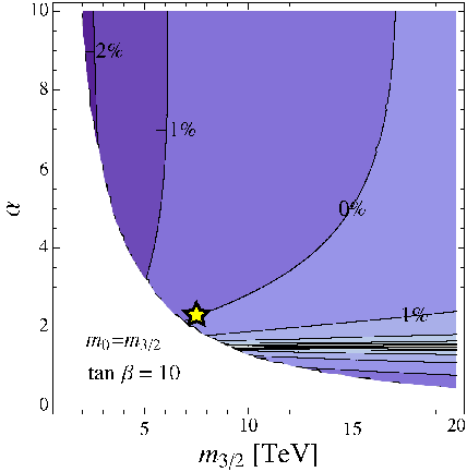
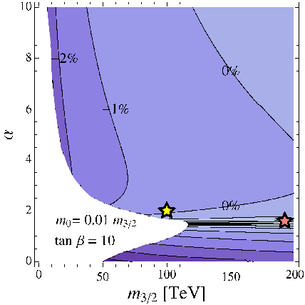
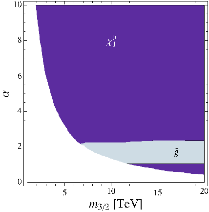
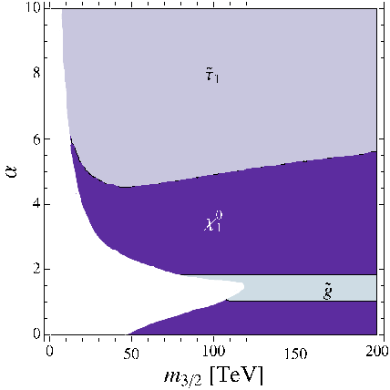
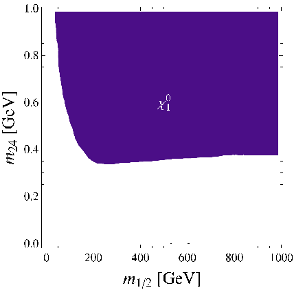
we fix $\sign\mu$ to be $+1$ . We conducted a scan over the continuous parameters $m_{3/2},~\alpha$ and $\tan\beta$ . It turns out that the deviation $\epsilon_{3}$ is almost independent of $\tan\beta$ . In figure 1 we therefore show $\epsilon_{3}$ for varying $m_{3/2}$ and $\alpha$ with fixed $\tan\beta=10$ . The white regions are excluded as follows: we take into account all points which are invalid according to SOFTSUSY [25] as well as collider bounds on sparticle masses.²² 2 Here we require that the lightest Higgs mass be above $112\>\text{Ge\kern-0.59998ptV}$ rather than above $114.4\>\text{Ge\kern-0.59998ptV}$ , since the theoretical error on the Higgs mass is about $2-3\>\text{Ge\kern-0.59998ptV}$ . Further, we are using version 3.0.9 of SOFTSUSY with a top quark mass of $173.1\>\text{Ge\kern-0.59998ptV}$ and $\alpha_{s}=0.1176$ . This implies a minimal value of $m_{3/2}\gtrsim 7\>\text{Te\kern-0.59998ptV}$ in order to be consistent with precision gauge coupling unification. At smaller values of $m_{3/2}$ the lighter chargino is below its experimental limit. Also shown in figure 1 are the corresponding LSPs.

To see the impact of smaller $m_{0}$ let us also consider the case where not only the gaugino masses but also the scalar masses are suppressed against the gravitino mass, e.g. $m_{0}^{\boldsymbol{16}}=\tfrac{1}{100}m_{3/2}$ . The corresponding plots are also shown in figure 1. Sample spectra for the two cases can be found in table 1.

While this paper is mainly concerned with precision gauge coupling unification, there are circumstances under which positive values of $\epsilon_{3}$ might also be interesting. Let us briefly discuss an example. If one is to accommodate negative $\epsilon_{3}$ in a concrete model, as it occurs in the ‘usual’ scenarios, one needs to have colored states lighter than the GUT scale. The most straightforward possibility for such states are the Higgs triplet partners (see e.g. [26]). However, there are tight constraints on the masses of such states coming from proton decay as such triplets induce dangerous dimension five operators, which disfavor this possibility. On the other hand, a positive $\epsilon_{3}$ would allow for color triplets which are substantially heavier than $M_{\mathrm{GUT}}$ , thus ameliorating the problems with dimension five operators. For example in SU(5) the contribution to $\epsilon_{3}$ of the color triplet Higgs is given by [27]

{\epsilon}_{3}^{\text{Higgs}}={3{\alpha_{\mathrm{GUT}}}\over 5\pi}\log\Big|{\widetilde{M_{t}}\over M_{\text{GUT}}}\Big|

(7)

with $\widetilde{M_{t}}$ the effective mass of the Higgs triplet. Hence for positive $\epsilon_{3}$ the triplet Higgs can naturally be heavier than $M_{\text{GUT}}$ (see e.g. [28] for a discussion on proton stability and an upper bound on $\widetilde{M_{t}}$ ). In scenarios with positive $\epsilon_{3}$ the gluino becomes even lighter. Sample spectra with $\epsilon_{3}=0.02$ are shown in table 2.

3.2 Non-singlet $\boldsymbol{F}$ -terms

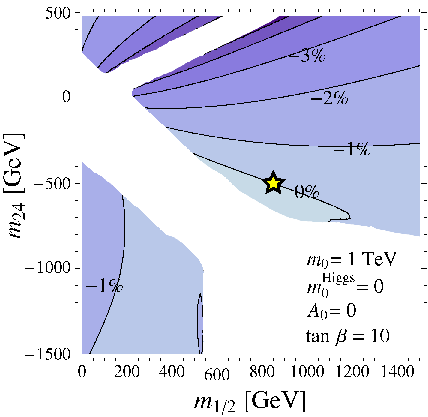
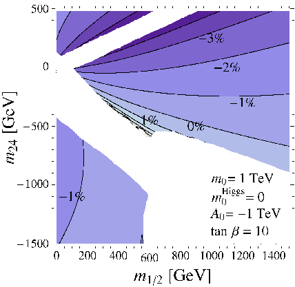
Another possible source for non-universal gaugino masses is to have non-singlet chiral fields which break supersymmetry by $F$ -term vacuum expectation values. These fields have to transform as the symmetric product of two adjoint representations of the GUT group, but not necessarily as singlets. For concreteness we focus here on SU(5) GUTs. In the following we concentrate on the two smallest possible representations for the supersymmetry breaking fields, which are simply the singlet and the $\boldsymbol{24}$ -plet. Including also the $\boldsymbol{75}$ and $\boldsymbol{200}$ would of course widen the available parameter space. Similar relations hold for SO(10).

The high-scale mass patterns of the gauginos of SU(3)_C, SU(2)_L and U(1)_Y turn out to be given as linear combinations of singlet ( $m_{1/2}$ ) and $\boldsymbol{24}$ -plet ( $m_{24}$ ) contributions [29],

$\displaystyle M_{1}$	$\displaystyle=$	$\displaystyle m_{1/2}-\tfrac{1}{2}\,m_{24}\;,$
$\displaystyle M_{2}$	$\displaystyle=$	$\displaystyle m_{1/2}-\tfrac{3}{2}\,m_{24}\;,$
$\displaystyle M_{3}$	$\displaystyle=$	$\displaystyle m_{1/2}+m_{24}\;.$	(8)

In figure 2 we show $\epsilon_{3}$ as a function of the two gaugino mass parameters $m_{1/2}$ and $m_{24}$ for fixed $m_{0}$ , $m_{0}^{\text{Higgs}}$ , $A_{0}$ and $\tan\beta$ . We find that in the allowed regions $-0.04\lesssim\epsilon_{3}\lesssim 0.03$ . The white regions are again excluded. The excluded regions are mainly due to the Higgs LEP bound. A sample spectrum is shown in table 1.

3.3 GMSB with Higgs messenger mixing

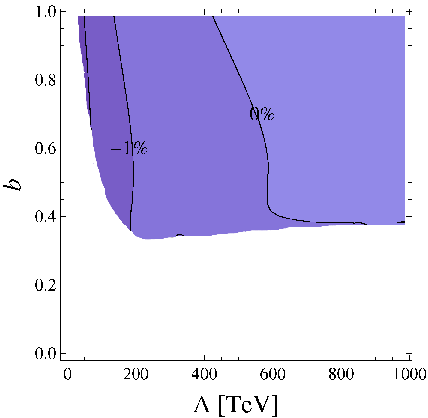
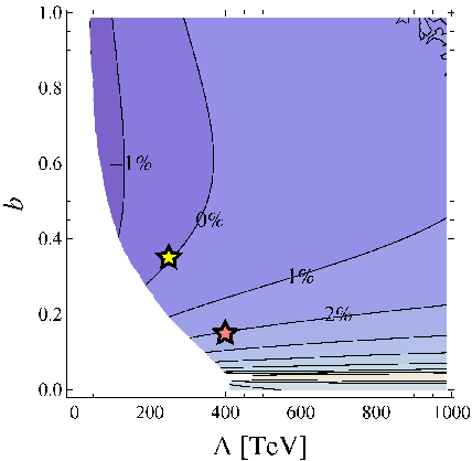
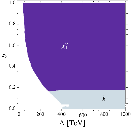
As a last example of a supersymmetry breaking mechanism which can lead to precision gauge coupling unification let us look at a particular version of gauge mediation [30, 31, 32]. The boundary conditions at the messenger scale $M\sim M_{\text{GUT}}$ are determined by five SUSY breaking parameters, $\Lambda\sim 10^{5}\>\text{Ge\kern-0.59998ptV}$ , $a\sim b\sim 0.01-0.1$ , $\mu$ and $B\mu$ . In addition a $D$ -term contribution is needed in order to obtain a phenomenologically acceptable theory [32]. The boundary conditions for the gauginos and scalars at the scale $M$ read


$\displaystyle M_{1}$	$\displaystyle=$	$\displaystyle\frac{3}{5}\frac{\alpha_{1}(M)}{4\pi}\Lambda\,\left(1+\frac{20}{3}b^{2}\right)\;,$	(9a)
$\displaystyle M_{2}$	$\displaystyle=$	$\displaystyle\frac{\alpha_{2}(M)}{4\pi}\Lambda\,\left(1+4b^{2}\right)\;,$	(9b)
$\displaystyle M_{3}$	$\displaystyle=$	$\displaystyle\frac{\alpha_{3}(M)}{\pi}\Lambda\,b^{2}\;,$	(9c)
$\displaystyle\widetilde{m}^{2}$	$\displaystyle=$	$\displaystyle 2\,\Lambda^{2}\,\bigg\{C_{1}\,\left(\frac{\alpha_{1}(M)}{4\pi}\right)^{2}\left(\frac{3}{5}+\frac{2}{5}a^{2}+4b^{2}\right)+C_{2}\,\left(\frac{\alpha_{2}(M)}{4\pi}\right)^{2}\left(1+4b^{2}\right)$	(9d)
		$\displaystyle\hphantom{2\, \Lambda^2\, \bigg\lx@text@lbrace}{}+C_{3}\,\left(\frac{\alpha_{3}(M)}{4\pi}\right)^{2}\left(a^{2}+4b^{2}\right)\bigg\}$	(9d)

with $C_{1}=\tfrac{3}{5}Y^{2}$ , $C_{2}=\tfrac{3}{4}$ for weak doublets and zero otherwise and $C_{3}=\tfrac{4}{3}$ for color triplets and zero otherwise. The additional $D$ -term contributions to the scalar masses are parameterized as

\delta_{D}\,\widetilde{m}^{2}~=~d\,Q_{a}^{X}\,M_{2}^{2}

(10)

with $d$ an arbitrary parameter of order one and $Q_{a}^{X}$ the U(1)_X charge of the field with label $a$ . In the following we will assume that $Q_{a}^{X}$ is 1 for the matter fields and -2 for the Higgs fields [32].

In figure 3 we show again the contours of different $\epsilon_{3}$ for the boundary conditions (9) at $M=M_{\text{GUT}}$ and $a=0.01$ , $A_{0}=0$ , $\tan\beta=10$ and $d=0$ or $d=1$ . In the region with small values of $b$ the gluino is the NLSP with the gravitino being the LSP and $\epsilon_{3}$ is positive. A sample spectrum is shown in table 2. Precision gauge coupling can be achieved for larger values of $b$ where the neutralino is the NLSP. A sample spectrum is shown in table 1.

4 Phenomenological implications

4.1 Prospects for the LHC

Let us now briefly comment on possible phenomenological implications of the requirement of precision gauge coupling unification. Sample spectra for the considered models are shown in table 1. One common feature of the models which admit precision gauge coupling unification seems to be that the gauginos are rather light while the scalars are typically somewhat heavier. It is therefore well possible that the gauginos are within the kinematical reach of the LHC while the scalars are not. At the LHC one would then expect that supersymmetric particles are mainly produced via gluino pair production, resulting in a signature with at least four jets plus missing energy. With an integrated luminosity of $100\,\mathrm{fb}^{-1}$ the LHC could probe gluino masses up to $\sim 2\>\text{Te\kern-0.59998ptV}$ [33]. As the squarks are heavier than the gluinos, the gluinos can either three-body decay via a virtual squark or two-body loop decay (for branching ratios see e.g. [34, 35]). The latter process is usually suppressed. As can be seen in table 1 the lighter stop is the lightest among the squarks, implying that the gluino decays will produce a high multiplicity of top quarks [33], if kinematically accessible. To summarize, squarks may be so heavy that they cannot be directly produced, in which case their masses have to be reconstructed by investigating the gluino decay processes, where they appear as intermediate states.

For positive $\epsilon_{3}$ the gluino is likely to be the lightest MSSM superpartner, in which case it may be long-lived. Depending on the lifetime the gluino hadronizes, travels macroscopic distances and might even escape the detector (see e.g. [36]). Potential signatures of such a scenario could therefore be displaced vertices or metastable R-hadrons which could be stopped in- or outside the detector. In any case the missing energy signature for SUSY is not present in such a scenario.

4.2 Further comments on scenarios with a low gluino mass

As is well known, scenarios with low gluino masses can also be interesting in the context of the little hierarchy problem. This is because the gluino mass has the largest impact on the Higgs mass parameters (cf. [37]). Given a specific measure of “fine-tuning” one also finds that low gluino masses increase naturalness (cf. e.g. [38, 39] for recent discussions). On the other hand, one should also mention that a large gluino mass has the virtue that the supersymmetric flavor problem gets ameliorated by flavor-universal contributions from the gluino in the renormalization group [40].

	$m_{0}=m_{3/2}$	$m_{0}=0.01\,m_{3/2}$	non-singlet	GMSB
$m_{h^{0}}$	121 GeV	115 GeV	115 GeV	116 GeV
$m_{H^{0}}$	5.59 TeV	1.31 TeV	1.21 TeV	1.39 TeV
$m_{A^{0}}$	5.59 TeV	1.31 TeV	1.21 TeV	1.39 TeV
$m_{H^{+}}$	5.59 TeV	1.31 TeV	1.21 TeV	1.39 TeV
$m_{\widetilde{u}_{\mathrm{L}\,1/2}}$	7.37 TeV	1.55 TeV	1.57 TeV	2.02 TeV
$m_{\widetilde{u}_{\mathrm{R}\,1/2}}$	7.42 TeV	1.42 TeV	1.23 TeV	1.62 TeV
$m_{\widetilde{d}_{\mathrm{L}\,1/2}}$	7.41 TeV	1.55 TeV	1.57 TeV	2.02 TeV
$m_{\widetilde{d}_{\mathrm{R}\,1/2}}$	7.42 TeV	1.23 TeV	1.20 TeV	1.53 TeV
$m_{\widetilde{t}_{1}}$	5.89 TeV	932 GeV	743 GeV	1.18 TeV
$m_{\widetilde{t}_{2}}$	6.66 TeV	1.36 TeV	1.41 TeV	1.86 TeV
$m_{\widetilde{b}_{1}}$	6.66 TeV	1.22 TeV	1.19 TeV	1.52 TeV
$m_{\widetilde{b}_{2}}$	7.39 TeV	1.15 TeV	1.40 TeV	1.85 TeV
$m_{\widetilde{e}_{\mathrm{L}\,1/2}}$	7.48 TeV	1.56 TeV	1.45 TeV	1.81 TeV
$m_{\widetilde{e}_{\mathrm{R}\,1/2}}$	7.49 TeV	1.42 TeV	1.08 TeV	1.44 TeV
$m_{\widetilde{\nu}_{\mathrm{L}\,1/2}}$	7.48 TeV	1.55 TeV	1.45 TeV	1.81 TeV
$m_{\widetilde{\tau}_{1}}$	7.45 TeV	1.55 TeV	1.07 TeV	1.43 TeV
$m_{\widetilde{\tau}_{2}}$	7.47 TeV	1.58 TeV	1.45 TeV	1.81 TeV
$m_{\widetilde{\nu}_{\tau_{L}}}$	7.46 TeV	1.55 TeV	1.44 TeV	1.81 TeV
$m_{\widetilde{g}}$	128 GeV	793 GeV	862 GeV	828 GeV
$m_{\chi_{1}^{0}}$	117 GeV	583 GeV	467 GeV	346 GeV
$m_{\chi_{2}^{0}}$	118 GeV	592 GeV	644 GeV	922 GeV
$m_{\chi_{1}^{\pm}}$	118 GeV	591 GeV	643 GeV	922 GeV
$m_{\chi_{3}^{0}}$	5.65 TeV	1.29 TeV	645 GeV	1.55 TeV
$m_{\chi_{4}^{0}}$	5.65 TeV	1.46 TeV	1.30 TeV	1.55 TeV
$m_{\chi_{2}^{\pm}}$	5.68 TeV	1.29 TeV	1.30 TeV	1.56 TeV
$M_{\mathrm{GUT}}$	$2.59\cdot 10^{16}$ GeV	$1.54\cdot 10^{16}$ GeV	$1.42\cdot 10^{16}$ GeV	$1.50\cdot 10^{16}$ GeV

Table 1: Sample spectra with vanishing

\epsilon_{3}

for the different cases. For the case ‘

m_{0}=m_{3/2}

’ (‘

m_{0}=0.01\,m_{3/2}

’) we choose

m_{3/2}=7.5

TeV (100 TeV),

\alpha=2.3

(2.0) and

\tan\beta=10

. In the case ‘non-singlet’ we have

m_{1/2}=848.5\>\text{Ge\kern-0.59998ptV}

m_{24}=-500\>\text{Ge\kern-0.59998ptV}

m_{0}=1\>\text{Te\kern-0.59998ptV}

A_{0}=0

and

\tan\beta=10

. For ‘GMSB’ we have

a=0.01

b=0.32

A_{0}=0

\Lambda=250\>\text{Te\kern-0.59998ptV}

d=1

and

\tan\beta=10

. The lightest neutralino turns out to be mainly bino in the cases ‘

m_{0}=m_{3/2}

’, ‘non-singlet’ and ‘GMSB’ while it is mainly Higgsino in the case ‘

m_{0}=0.01\,m_{3/2}

’.

	$m_{0}=0.01\,m_{3/2}$	GMSB
$m_{h^{0}}$	117 GeV	115 GeV
$m_{H^{0}}$	2.23 TeV	1.60 TeV
$m_{A^{0}}$	2.23 TeV	1.60 TeV
$m_{H^{+}}$	2.24 TeV	1.61 TeV
$m_{\widetilde{u}_{\mathrm{L}\,1/2}}$	2.63 TeV	2.36 TeV
$m_{\widetilde{u}_{\mathrm{R}\,1/2}}$	2.50 TeV	1.67 TeV
$m_{\widetilde{d}_{\mathrm{L}\,1/2}}$	2.64 TeV	2.37 TeV
$m_{\widetilde{d}_{\mathrm{R}\,1/2}}$	2.12 TeV	1.52 TeV
$m_{\widetilde{t}_{1}}$	1.70 TeV	1.07 TeV
$m_{\widetilde{t}_{2}}$	2.29 TeV	2.18 TeV
$m_{\widetilde{b}_{1}}$	2.10 TeV	1.51 TeV
$m_{\widetilde{b}_{2}}$	2.29 TeV	2.17 TeV
$m_{\widetilde{e}_{\mathrm{L}\,1/2}}$	2.86 TeV	2.37 TeV
$m_{\widetilde{e}_{\mathrm{R}\,1/2}}$	3.04 TeV	1.81 TeV
$m_{\widetilde{\nu}_{\mathrm{L}\,1/2}}$	2.86 TeV	2.36 TeV
$m_{\widetilde{\tau}_{1}}$	2.85 TeV	1.80 TeV
$m_{\widetilde{\tau}_{2}}$	3.02 TeV	2.36 TeV
$m_{\widetilde{\nu}_{\tau_{L}}}$	2.85 TeV	2.36 TeV
$m_{\widetilde{g}}$	385 GeV	301 GeV
$m_{\chi_{1}^{0}}$	963 GeV	379 GeV
$m_{\chi_{2}^{0}}$	968 GeV	1.14 TeV
$m_{\chi_{1}^{\pm}}$	974 GeV	1.14 TeV
$m_{\chi_{3}^{0}}$	2.21 TeV	1.63 TeV
$m_{\chi_{4}^{0}}$	2.76 TeV	1.64 TeV
$m_{\chi_{2}^{\pm}}$	2.21 TeV	1.64 TeV
$M_{\mathrm{GUT}}$	$1.33\cdot 10^{16}\>\text{Ge\kern-0.59998ptV}$	$1.39\cdot 10^{16}\>\text{Ge\kern-0.59998ptV}$

Table 2: Sample spectra with

\epsilon_{3}=0.02

. In the case ‘

m_{0}=0.01\,m_{3/2}

’ we choose

m_{3/2}=200\>\text{Te\kern-0.59998ptV}

\alpha=1.615

and

\tan\beta=10

while in the case ‘GMSB’ we have

a=0.01

b=0.145

A_{0}=0

\Lambda=400\>\text{Te\kern-0.59998ptV}

d=1

and

\tan\beta=10

. In both examples the gluino is the lightest MSSM superparticle, such that dark matter has to be composed of some other, probably very weakly coupled particle(s).

5 Summary

We have shown that it is possible to have precision gauge coupling unification in the MSSM without invoking high-scale thresholds. This can be simply achieved in schemes in which the gaugino masses are non-universal at (or slightly below) the GUT scale. Such non-universal gaugino masses are consistent with unified theories. They occur, for instance, in settings in which the tree-level value of the gaugino masses are suppressed such that quantum corrections, such as ‘anomaly mediated’ contributions, become important. They can also be obtained in settings in which supersymmetry is broken by a field furnishing a non-trivial GUT representation as well as in GMSB with Higgs-messenger mixing. We also note that $\epsilon_{3}$ can be positive.

Interestingly, there is a correlation between low fine-tuning and precision gauge coupling unification. Both features can be achieved by having a rather light gluino. The emerging schemes have the virtue that it will be relatively easy for the LHC to produce gluinos copiously. On the other hand, squarks may turn out to be too heavy to be directly produced such that one would have to reconstruct their masses by analyzing gluino decays. There is also the possibility of displaced vertices from gluino decay as well as meta-stable gluino bound states stopped in the detector.

Acknowledgments.

We would like to thank G. Ross for useful discussions. S.R. would like to acknowledge partial support from DOE grant DOE/ER/01545-883. This research was supported by the DFG cluster of excellence Origin and Structure of the Universe and the SFB-Transregio 27 ”Neutrinos and Beyond” by Deutsche Forschungsgemeinschaft (DFG). One of us (M.R.) would like to thank the Aspen Center for Physics, where some of this work has been carried out, for hospitality and support. K.S.-H. would like to thank LPSC Grenoble for hospitality and support.

References

[1] S. Dimopoulos, S. Raby, and F. Wilczek, Phys. Rev. D24 (1981), 1681–1683.
[2] S. Dimopoulos and H. Georgi, Nucl. Phys. B193 (1981), 150.
[3] L. E. Ibáñez and G. G. Ross, Phys. Lett. B105 (1981), 439.
[4] M. B. Einhorn and D. R. T. Jones, Nucl. Phys. B196 (1982), 475.
[5] W. J. Marciano and G. Senjanovic, Phys. Rev. D25 (1982), 3092.
[6] M. L. Alciati, F. Feruglio, Y. Lin, and A. Varagnolo, JHEP 03 (2005), 054, [hep-ph/0501086].
[7] Particle Data Group, C. Amsler et al., Phys. Lett. B667 (2008), 1.
[8] L. E. Ibáñez, D. Lüst, and G. G. Ross, Phys. Lett. B272 (1991), 251–260, [hep-th/9109053].
[9] L. E. Ibáñez and D. Lüst, Nucl. Phys. B382 (1992), 305–364, [hep-th/9202046].
[10] H. P. Nilles and S. Stieberger, Phys. Lett. B367 (1996), 126–133, [hep-th/9510009].
[11] L. J. Hall and Y. Nomura, Phys. Rev. D64 (2001), 055003, [hep-ph/0103125].
[12] A. Hebecker and M. Trapletti, Nucl. Phys. B713 (2005), 173–203, [hep-th/0411131].
[13] M. S. Carena, S. Pokorski, and C. E. M. Wagner, Nucl. Phys. B406 (1993), 59–89, [hep-ph/9303202].
[14] L. Roszkowski and M. A. Shifman, Phys. Rev. D53 (1996), 404–412, [hep-ph/9503358].
[15] O. Loaiza-Brito, J. Martin, H. P. Nilles, and M. Ratz, AIP Conf. Proc. 805 (2006), 198–204, [hep-th/0509158].
[16] K. Choi, A. Falkowski, H. P. Nilles, and M. Olechowski, Nucl. Phys. B718 (2005), 113–133, [hep-th/0503216].
[17] K. Choi, K. S. Jeong, and K.-i. Okumura, JHEP 09 (2005), 039, [hep-ph/0504037].
[18] A. Falkowski, O. Lebedev, and Y. Mambrini, JHEP 11 (2005), 034, [hep-ph/0507110].
[19] V. Löwen and H. P. Nilles, Phys. Rev. D77 (2008), 106007, [0802.1137].
[20] O. Lebedev, H. P. Nilles, and M. Ratz, Phys. Lett. B636 (2006), 126–131, [hep-th/0603047].
[21] O. Lebedev, V. Löwen, Y. Mambrini, H. P. Nilles, and M. Ratz, JHEP 02 (2007), 063, [hep-ph/0612035].
[22] A. B. Lahanas and K. Tamvakis, Phys. Lett. B348 (1995), 451–456, [hep-ph/9412281].
[23] K. Choi and H. P. Nilles, JHEP 04 (2007), 006, [hep-ph/0702146].
[24] V. Löwen and H. P. Nilles, (2009), 0907.4983.
[25] B. C. Allanach, Comput. Phys. Commun. 143 (2002), 305–331, [hep-ph/0104145].
[26] B. Dundee, S. Raby, and A. Wingerter, (2008), 0805.4186.
[27] V. Lucas and S. Raby, Phys. Rev. D54 (1996), 2261–2272, [hep-ph/9601303].
[28] R. Dermís̆ek, A. Mafi, and S. Raby, Phys. Rev. D63 (2001), 035001, [hep-ph/0007213].
[29] K. Huitu, Y. Kawamura, T. Kobayashi, and K. Puolamaki, Phys. Rev. D61 (2000), 035001, [hep-ph/9903528].
[30] S. Raby, Phys. Rev. D56 (1997), 2852–2860, [hep-ph/9702299].
[31] S. Raby, Phys. Lett. B422 (1998), 158–162, [hep-ph/9712254].
[32] S. Raby and K. Tobe, Nucl. Phys. B539 (1999), 3–22, [hep-ph/9807281].
[33] J. D. Wells, (2003), hep-ph/0306127.
[34] R. Barbieri, G. Gamberini, G. F. Giudice, and G. Ridolfi, Nucl. Phys. B301 (1988), 15.
[35] H. Baer, X. Tata, and J. Woodside, Phys. Rev. D42 (1990), 1568–1576.
[36] W. Kilian, T. Plehn, P. Richardson, and E. Schmidt, Eur. Phys. J. C39 (2005), 229–243, [hep-ph/0408088].
[37] G. L. Kane, J. D. Lykken, B. D. Nelson, and L.-T. Wang, Phys. Lett. B551 (2003), 146–160, [hep-ph/0207168].
[38] I. Gogoladze, M. U. Rehman, and Q. Shafi, Phys. Rev. D80 (2009), 105002, [0907.0728].
[39] D. Horton and G. G. Ross, (2009), 0908.0857.
[40] M. Dine, A. Kagan, and S. Samuel, Phys. Lett. B243 (1990), 250–256.