A model for right-handed neutrino magnetic moments
Abstract
A simple extension of the Standard Model providing Majorana magnetic moments to right-handed neutrinos is presented. The model contains, in addition to the Standard Model particles and right-handed neutrinos, just a singly charged scalar and a vector-like charged fermion. The phenomenology of the model is analysed and its implications in cosmology, astrophysics and lepton flavour violating processes are extracted. If light enough, the charged particles responsible for the right-handed neutrino magnetic moments could copiously be produced at the LHC.
Keywords:
Neutrinos, magnetic moments, effective Lagrangian, LHCPACS
14.60.St, 13.35.Hb, 13.15.+g, 13.66.Hk1 Introduction
In ref. [1] we studied the most general effective Lagrangian built with the Standard Model (SM) fields plus right-handed neutrinos up to operators of dimension five. We found this Lagrangian contains only three nonrenormalizable operators, one of them being the well known Weinberg operator [2] which only involves the SM lepton doublets and the Higgs doublet. The other two contain an interaction of right-handed neutrinos with the SM Higgs doublet and a Majorana electroweak moment for the right-handed neutrinos. This last operator is particularly interesting and can have a variety of phenomenological consequences in cosmology, astrophysics and at colliders [1]. Of course, it is interesting to have explicit models in which these nonrenormalizable interactions arise naturally because one can use them to check the general features of the effective Lagrangian approach and extend them outside the realm of validity of the effective field theory. This is especially important if the particles responsible for the new interactions are light enough as to be produced at the next generation of colliders.
Here we present a very simple model which gives rise to right-handed neutrino electroweak moments; it includes, in addition to the SM fields and the right-handed neutrinos, a charged scalar singlet and a charged singlet vector-like fermion. We obtain the tree level and one-loop contributions to the dimension five effective Lagrangian, and in particular we compute the contribution to the right-handed neutrino electroweak moments. We perform a thorough phenomenological analysis of the model, paying special attention to the case in which the new charged particles are light enough to be produced at the Large Hadron Collider (LHC). Thus, in section 2 we define the model and compute the one-loop contribution to the electroweak moment of right-handed neutrinos. The simplest version of the model, in which several couplings are set to zero by using global symmetries, contains stable charged massive particles (CHAMPs) which are strongly disfavoured from cosmological and astrophysical considerations. To avoid such problems we extend minimally the model by allowing a soft breaking of the symmetries, which is enough to induce CHAMP decays; such decays are studied in section 2.3. The model also induces some tree-level lepton flavour violating (LFV) processes like which are studied in section 2.4. In section 3 we discuss briefly the one-loop contributions of the model to the effective Higgs- operator. In section 4 we compute the production cross section of the charged particles at the LHC and discuss their observability as a function of their masses. Finally, in section 5 we present our conclusions.
2 The model
As discussed in ref. [1] the most general dimension five interactions among SM fields and three right-handed neutrinos can be written as11 1 The reader should note a difference in notation respect to [1], where we used to denote the neutrino flavor eigenfields. As in the present work we are not going to discuss the diagonalisation of the neutrino mass matrices we will just use to represent the flavor eigenfields.
| (1) |
where denotes the left-handed lepton isodoublet, and the corresponding right-handed isosinglets, and the scalar isodoublet (family and gauge indices will be suppressed when no confusion can arise). The charge-conjugate fields are defined as and where acts on the indices. The hypercharges assignments are , , , . The and gauge fields are denoted by and respectively (gluon and quarks fields will not be needed in the situations considered below). The couplings , , have dimension of inverse mass, which is associated with the scale of the heavy physics responsible for the corresponding operator. , and are complex symmetric matrices in flavour space, while is a complex antisymmetric matrix proportional to the right-handed neutrino electroweak moments.
The different terms in eq. (1) and their phenomenological consequences were discussed in [1]. Here we are more interested in models that could give rise to . This can only occur at the one-loop level and the models should necessarily involve either a scalar-fermion pair with opposite (non-zero) hypercharges and having Yukawa couplings with both and , or a vector-fermion pair with the same properties. Here we will consider only the first (simpler) possibility. Thus we enlarge the SM by adding a negatively charged scalar singlet , , and one negatively charged vector-like fermion (two chiralities and no generation indices) also with .
We can then write the Lagrangian as
| (2) |
where is the SM Lagrangian while the new physics Lagrangian, , collects all the terms containing any of the new particles, including among them the right-handed neutrinos. We write as
| (3) |
with the Yukawa couplings of charged leptons which are completely general matrices in flavour space; the dots represent SM gauge boson, Higgs boson and quark kinetic terms, quark Yukawa interactions and the SM Higgs potential. We divide the new physics contribution, , in different terms:
| (4) |
describes the kinetic terms of the new particles
| (5) |
with the Majorana mass term of right-handed neutrinos, which is a complex symmetric matrix in flavour space. contains the standard Yukawa interactions of right-handed neutrinos and the Yukawa couplings of right-handed neutrinos with the particles needed to generate the electroweak moments:
| (6) |
is a general complex matrix and, if there is just one , and are vectors in generation space. The contributions to the scalar potential are
| (7) |
Where is the vacuum expectation value of the Higgs doublet, , and the ’s are quartic scalar couplings. We assume and to insure global (tree-level) stability, as well as in order to preserve . It is important to remark that with only one Higgs doublet there cannot be trilinear couplings between the doublet and the singlet, . Then, the potential has two independent symmetries, one for the singlet and one for the doublet.
In addition, the SM symmetries allow the following Yukawa couplings and mass terms
| (8) |
which can be set to zero by imposing a discrete symmetry which affects only the new particles
| (9) |
In this case all low-energy physics effects will be loop generated[3]. Notice that the resulting Lagrangian has a larger continuous symmetry
| (10) |
which is not anomalous, therefore there is a charge, carried only by and which is exactly conserved. In that case, the lightest of the or will be completely stable becoming a CHAMP, which could create serious problems in standard cosmology scenarios. However, such problems can easily be evaded by allowing some of the terms in eq. (8). We will return to this issue after verifying that the model indeed generates a right-handed neutrino magnetic moment.
2.1 The magnetic moment
In the model considered we have two diagrams, depicted in figure 1, contributing to the Majorana electroweak moment: a) loop with the gauge boson attached to the and b) loop with the gauge boson attached to the scalar .

For we can neglect all external momenta and masses and the calculation of the diagrams simplifies considerably. The final result can be cast as a contribution to the effective magnetic moment operator in eq. (1). We find
| (11) |
with , the gauge coupling and
| (12) |
For an estimate we can take, for instance, , and while , then (for there will be a factor enhancement and for there will be a suppression by roughly a factor ); these values are in agreement with the estimates obtained using effective field theory. In terms of we have . Present bounds from LEP and Tevatron give , which imply . This can be compared with direct bounds that can be set on the right-handed neutrino electroweak moments derived in [1] . As expected, collider limits on production are much more restrictive than collider limits derived from the induced electroweak moment interaction. After all, the electroweak moment interaction is generated at one loop. However, if the right-handed neutrinos are relatively light (below ) bounds from transition magnetic moments coming from supernova cooling (which are ) or red giant cooling (which are for ) can be much stronger.
2.2 E or as CHAMPs
The model as described so far contains only the couplings necessary to generate the right-handed neutrino Majorana electroweak moments. But it is clear that the trilinear vertices and alone cannot induce decays for both the and the . The lightest of the two will remain stable and could then accumulate in the galaxy clusters, appearing as electrically charged dark matter. The idea that dark matter could be composed mostly of charged massive particles was proposed in [4, 5] and it is strongly constrained from very different arguments[6, 7, 8, 9, 10]. One might still consider the possibility of having massive stable or particles within the reach of the LHC, but with a cosmic abundance lower than the one required for dark matter. Unfortunately, such scenario seems also to be excluded: if one assumes, as in [4], that the ’s and ’s were produced in the early universe through the standard freeze-out mechanism [11], the bounds from interstellar calorimetry [10] and terrestrial searches for super-heavy nuclei [7, 8] completely close the window of under-TeV CHAMP abundances.
There is, however, a way to escape all these bounds. A recent paper [12] notes that CHAMPs, if very massive or carrying very small charges, are expelled from the galactic disk by the magnetic fields. That situation prevents any terrestrial or galactic detection and leaves room for CHAMPs to exist. The bound specifically states that particles with are depleted from the disk, and in fact our model (if we forbid the terms in eq. (8)) does not fix the hypercharge of and , so they can be millicharged. Unfortunately, this situation is not interesting for our purposes, for this kind of CHAMPs would give rise to very small neutrino magnetic moments and wouldn’t show up in the future accelerators, either due to their heavy masses or to their small couplings.
In conclusion, we need an additional mechanism for or decays. The easiest way to accomplish this is by allowing one or more of the couplings in eq. (8), which can be taken small, if needed, by arguing that (10) is an almost exact symmetry. We discuss one of the possibilities in section 2.3. The scenario of decaying CHAMPs has, on its own, a number of advantages and drawbacks. Some recent papers [13, 14] have pointed out that the presence of a massive, charged and colourless particle during the process of primordial nucleosynthesis might lead to an explanation for the cosmic lithium problem. Also, the decay of massive particles during nucleosynthesis could have a dramatic influence in the final abundances of primordial elements, which provides us with bounds on the lifetime and abundance of CHAMPs that could be useful.
2.3 Allowing for CHAMP decays
If the particles have to decay the global symmetry (10) has to be broken, and for that it is enough to allow some of the terms in eq. (8). For the sake of simplicity, we will consider only the case where the symmetry is softly broken by – mixing22 2 Since this choice breaks (10) softly, none of the other terms in eq. (8) need be introduced for the model to remain renormalizable.
| (13) |
This term will induce decays of into SM particles much like the heavy neutrino decays in seesaw models, since only this mixing links the to the SM degrees of freedom. After diagonalisation of the charged lepton mass matrix one obtains interactions that connect the to , and . As the current bound on heavy charged leptons require that , the and will be produced on-shell; the Higgs channel may or may not be open depending on the actual value of the Higgs and masses33 3 Note that, as is not broken, flavour-changing vertices involving a photon cannot appear at tree level; must be at least a one-loop effect, and thereby suppressed..
The , on the other hand, has to decay through the Yukawa vertices; either directly to if or to suppressed by the mixing . The simplest situation then arises if , for in that case the ’s will decay into on-shell ’s, which in turn will decay in the aforementioned way. In what remains, for simplicity, we shall restrict ourselves to this specific case.
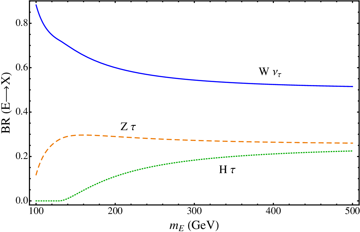
In figure 2 we present the branching ratios for the decays of the . As the decays are controlled by the would-be Goldstone part of the and (and the Higgs boson if allowed kinematically) they are always proportional to the Yukawa couplings of the charged leptons; therefore, if all the ’s are of the same order, the will decay mainly to the leptons of the third family. We can see that for relatively low masses the dominant channel is while for very large masses the ratios tend to the equivalent-Goldstone approximation: for the channel and for the and channels.
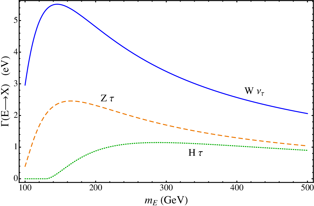
The decay rates of the fermion are presented in figure 3 for . Notice that the rates decrease for large . This is because the decays proceed through the mixing – and this is suppressed by factors ; thus the increase in phase space for large is compensated by these factors. For the chosen value of the decay widths are of the order of the eV. For widths of this order of magnitude the ’s will not be present at the time of primordial nucleosynthesis and will not affect it. Note, however, that the decay rates depend on , and is relatively free, thus the decay rates can vary in several orders of magnitude depending on the value of . For the CHAMPs will affect nucleosynthesis and, as commented above, might help to solve the cosmic lithium problem [13, 14]. We also require to avoid CHAMPs at the present epoch.
2.4 Lepton Flavour Violating processes
For general ’s and Yukawa couplings , family lepton flavour is not conserved; one might then worry about possible bounds set by processes like , or . We now determine whether the bounds on those rare processes can impose restrictions on the parameters of our model.
The easiest way to calculate the amplitudes for these processes is by using an effective Lagrangian obtained by integration of the field. This integration is performed by using the equations of motion for and expanding in powers of (for a detailed example of the integration of a singly charged scalar see [15]). One then obtains
| (14) |
which, after the use of the equations of motion and spontaneous symmetry breaking leads to a lepton flavour violating interaction of the gauge boson with left-handed charged leptons,
| (15) |
is a matrix in flavor space which is not, in general, diagonal; therefore, eq. (15) will induce processes such as and . Without loss of generality we can take diagonal with elements proportional to the charged lepton masses; then we can estimate the branching ratio for the process as
| (16) |
Our effective Lagrangian is an expansion in powers of which could be compensated, in part, by factors in the numerator; thus, for consistency, we should require which allows us to establish an upper bound for the branching ratio. Recalling also that the present limit on the mass of charged heavy leptons is around , and therefore we should have , we obtain
| (17) |
to be compared with present bounds44 4 All experimental limits are taken from[16]. which are of the order of . If we apply the same reasoning to we see that the branching ratio is enhanced by a factor
| (18) |
which is still under the present sensitivity for this ratio, which is about .
Another very restrictive process is , which is bounded at the level, . This limit will be improved in a close future by the MEG experiment by two orders of magnitude [17]. However, this process can only arise at one loop and it is suppressed by loop factors; therefore, we do not expect stringent bounds from it. The contributions to the oblique parameters are suppressed by powers of the fermions masses and are too small to be observed at the currently available precision.
Finally, – conversion in nuclei also provides strong limits in general; for instance, – conversion on gives . In our model, the process is induced by exactly the same interaction (15) that gives , and we again do not expect, at present, a strong bound from – conversion. However, given the future plans to improve the limits by several orders of magnitude, then perhaps – conversion will provide the best bound for LFV processes in this model. In any case, current data on LFV processes cannot constrain this mechanism for decays.
3 The mass and the effective Higgs boson interaction with
The model we have discussed contains several sources of lepton number non-conservation: the right-handed neutrino Majorana mass and the and couplings (if both of them are different from zero). Then it is interesting to ask what is the natural size of the right-handed neutrino Majorana masses, since, even if they are set to zero by hand, radiative corrections involving couplings that do not conserve lepton number will generate them. In fact, by removing the photon line in the diagrams that give rise to the electroweak moments, figure 1, one obtains a renormalization of the right-handed neutrino Majorana mass. The diagrams are logarithmically divergent and give corrections of the type
| (19) |
(if the scalar is much heavier than the , this contribution will have an extra suppression ). It is then natural to require . Of course these type of contributions can be renormalized into which, after all, is a free parameter of the theory.

In addition, similar diagrams with a vertex attached to the field (see figure 4) give a finite contribution to the operator that cannot be avoided. A simple calculation gives
| (20) |
where can be written in terms of , defined in eq. (12): . After spontaneous symmetry breaking this operator gives additional contributions to the right-handed Majorana neutrino mass
| (21) |
Therefore, at least, one should require
| (22) |
where we took . By taking smaller couplings, smaller right-handed neutrino masses would be natural (for instance for one obtains ).
4 The Model at colliders

In spite of the fact that the new particles are singlets and only have Yukawa couplings to right-handed neutrinos, they are charged and can be copiously produced at the LHC, if light enough (), through the Drell-Yan process.
The cross sections for proton-proton collisions can be computed in terms of the partonic cross sections using the parton distribution functions of the proton (for a very clear review see for instance [18]); in figure 5 we present the results55 5 We have used the CTEQ6M parton distribution sets [19]. One could also include next-to-leading-order corrections by multiplying by a -factor which typically would change cross sections by . Results have been checked against the CompHEP program [20, 21]. for the production total cross sections at the LHC ( as a function of the and masses, and (both represented by in the figure). Since the particles are produced by and exchange, there are no unknown free parameters except the masses of the particles. We see that cross sections from to are easily obtained for the production of for masses between and . For the same masses the production cross section for is roughly one order of magnitude smaller.
Once produced in pairs, the particles have to be detected and identified. The characteristic signatures for this identification are very different depending on the lifetimes of the particles, mostly because if the and are long-lived they can be tracked directly in the detectors or, at least, be identified through a displaced decay vertex. The parameter relevant for this behavior is , the mixing.
For , the ’s will have decay lengths roughly over centimeter66 6 Note that there’s room in the parameter space for this kind of effects even if one requires that CHAMPs do not affect the primordial nucleosynthesis, for if all the ’s will have decayed before nucleosynthesis., in fact, for , they will go through the detector and behave as a heavy ionizing particle. A lot of work has been carried to analyse the signatures of CHAMPs inside the detector (see, for example, [22], and [23] for a recent improvement), and also displaced vertices have been discussed (see, for example, [24, 25]). If the ’s will decay near the collision point and behave as a fourth generation charged lepton.
Discovering the ’s can be much harder, because they will be produced at a significantly lower rate and the signatures of their decays depend strongly on the details of the model. In the scenario, they will decay quickly into an and a heavy neutrino (at least if we want and large enough to have significant electroweak moments) and then one has to rely again on the detection of ’s unless the heavy neutrino provides a cleaner signal, which is unlikely. In any case, we think that the ’s, produced in a much greater number, should be considered the signature of this model, and perhaps the doorway to understand the and heavy neutrino decays.
5 Conclusions
We have presented a simple model that generates right-handed neutrino magnetic moments and studied its phenomenology. The simplest version of the model contains CHAMPs (charged massive stable particles) which could present some problems with standard cosmological scenarios. These problems can easily be evaded by allowing additional couplings in the Lagrangian. The model can then give rise to various LFV processes at tree level such as ; however, we have verified that the rates of these processes are strongly suppressed and are well below present and near-future experimental constraints.
The same interactions that generate the right-handed neutrino magnetic moments will also generate, at one loop, the last operator in eq. (1) which provides a lepton number non-conserving interaction between neutrinos and the SM Higgs boson. This interaction gives an additional contribution to the right-handed neutrino Majorana mass; it is also interesting because could lead to an invisible Higgs decay [1]. We have computed it and discussed some of its consequences.
Finally, since the particles responsible for the right-handed neutrino magnetic moment are charged, if light enough they can copiously be produced at the LHC through the Drell-Yan process. We found that the cross sections for Drell-Yan production of ’s range from to for masses between and . For the same range of masses the production cross section for is roughly one order of magnitude smaller.
In short, we showed that a very simple model giving rise to right-handed neutrino magnetic models compatible with all existing constraints can easily be constructed. If the right-handed neutrinos are relatively heavy () bounds on magnetic moments from red giants or supernovae do not apply [1] and the charged particles responsible for the magnetic moments could be light enough as to be produced and detected at the LHC.
Acknowledgments
This work has been supported in part by the Ministry of Science and Innovation (MICINN) Spain, under the grant number FPA2008-03373, by the “Generalitat Valenciana” grant PROMETEO/2009/128, by the European Union within the Marie Curie Research & Training Networks, MRTN-CT-2006-035482 (FLAVIAnet), and by the U.S. Department of Energy grant No. DE-FG03-94ER40837. A.A. is supported by the MICINN under the FPU program.
References
- [1] A. Aparici et al., Phys. Rev. D80 (2009) 013010, 0904.3244.
- [2] S. Weinberg, Phys. Rev. Lett. 43 (1979) 1566.
- [3] J. Wudka, J. Phys. G31 (2005) 1401.
- [4] A. De Rujula, S.L. Glashow and U. Sarid, Nucl. Phys. B333 (1990) 173.
- [5] S. Dimopoulos et al., Phys. Rev. D41 (1990) 2388.
- [6] J.L. Basdevant et al., Phys. Lett. B234 (1990) 395.
- [7] T.K. Hemmick et al., Phys. Rev. D41 (1990) 2074.
- [8] T. Yamagata, Y. Takamori and H. Utsunomiya, Phys. Rev. D47 (1993) 1231.
- [9] A. Gould et al., Phys. Lett. B238 (1990) 337.
- [10] R.S. Chivukula et al., Phys. Rev. Lett. 65 (1990) 957.
- [11] S. Wolfram, Phys. Lett. B82 (1979) 65.
- [12] L. Chuzhoy and E.W. Kolb, JCAP 0907 (2009) 014, 0809.0436.
- [13] K. Jedamzik, JCAP 0803 (2008) 008, 0710.5153.
- [14] K. Jedamzik, Phys. Rev. D77 (2008) 063524, 0707.2070.
- [15] M.S. Bilenky and A. Santamaria, Nucl. Phys. B420 (1994) 47, hep-ph/9310302.
- [16] Particle Data Group, C. Amsler et al., Phys. Lett. B667 (2008) 1.
- [17] MEG, S. Ritt, Nucl. Phys. Proc. Suppl. 162 (2006) 279.
- [18] J.M. Campbell, J.W. Huston and W.J. Stirling, Rept. Prog. Phys. 70 (2007) 89, hep-ph/0611148.
- [19] J. Pumplin et al., JHEP 07 (2002) 012, hep-ph/0201195.
- [20] CompHEP, E. Boos et al., Nucl. Instrum. Meth. A534 (2004) 250, hep-ph/0403113.
- [21] A. Pukhov et al., CompHEP: A package for evaluation of Feynman diagrams and integration over multi-particle phase space. User’s manual for version 33, 1999, hep-ph/9908288, INP-MSU-98-41-542. 126pp. User’s manual for version 33.
- [22] M. Fairbairn et al., Phys. Rept. 438 (2007) 1, hep-ph/0611040.
- [23] J. Chen and T. Adams, (2009), 0909.3157.
- [24] R. Franceschini, T. Hambye and A. Strumia, Phys. Rev. D78 (2008) 033002, 0805.1613.
- [25] F. de Campos et al., Phys. Rev. D79 (2009) 055008, 0809.0007.