New insights into the neutron electric dipole moment

K. Ottnad Address: Helmholtz-Institut für Strahlen- und Kernphysik (Theorie) and Bethe Center for Theoretical Physics
Universität Bonn, D-53115 Bonn, Germany B. Kubis Address: Helmholtz-Institut für Strahlen- und Kernphysik (Theorie) and Bethe Center for Theoretical Physics
Universität Bonn, D-53115 Bonn, Germany U.-G. Meißner Address: Helmholtz-Institut für Strahlen- und Kernphysik (Theorie) and Bethe Center for Theoretical Physics
Universität Bonn, D-53115 Bonn, Germany Address: Institut für Kernphysik, Jülich Center for Hadron Physics and Institute for Advanced Simulation
Forschungszentrum Jülich, D-52425 Jülich, Germany F.-K. Guo Address: Institut für Kernphysik, Jülich Center for Hadron Physics and Institute for Advanced Simulation
Forschungszentrum Jülich, D-52425 Jülich, Germany

Abstract

We analyze the CP-violating electric dipole form factor of the nucleon in the framework of covariant baryon chiral perturbation theory. We give a new upper bound on the vacuum angle, $|\theta_{0}|\lesssim 2.5\cdot 10^{-10}$ . The quark mass dependence of the electric dipole moment is discussed and compared to lattice QCD data. We also perform the matching between its representations in the three- and two-flavor theories.

Keywords:

CP violation, chiral Lagrangians, neutron electric dipole moment

PACS

11.30.Er , 12.39.Fe , 14.20.Dh

HISKP-TH-09/32, FZJ-IKP-TH-2009-33

, , ,

1. The neutron electric dipole moment (nEDM) is a sensitive probe of CP violation in the Standard Model and beyond. The current experimental limit $d_{n}\leq 2.9\cdot 10^{-26}\,e\,{\rm cm}$ [1] is still orders of magnitude larger than the Standard Model prediction due to weak interactions. However, in QCD the breaking of the $U(1)_{A}$ anomaly allows for strong CP violation, which is parameterized through the vacuum angle $\theta_{0}$ . Therefore, an upper bound on $d_{n}$ allows to constrain the magnitude of $\theta_{0}$ . New and on-going experiments with ultracold neutrons strive to improve these bounds even further, see e.g. [2] for a very recent review. On the theoretical side, first full lattice QCD calculations of the neutron electric dipole moment are becoming available [3, 4, 5]. These require a careful study of the quark mass dependence of the nEDM to connect to the physical light quark masses. In addition, CP-violating atomic effects can be sensitive to the nuclear Schiff moment, which receives a contribution from the radius of the nucleon electric dipole form factor, see e.g. [6]. It is thus of paramount interest to improve the existing calculations of these fundamental quantities in the framework of chiral perturbation theory. In [7], the electric dipole moments of the neutron and the $\Lambda$ were calculated within the framework of $U(3)_{L}\times U(3)_{R}$ heavy-baryon chiral perturbation theory and an estimate for $\theta_{0}$ was given (for earlier works utilizing chiral Lagrangians, see [8, 9]). In [10], the electric dipole form factor of the nucleon was analyzed to leading one-loop accuracy in chiral $SU(2)$ , thus in that calculation the form factor originates entirely from the pion cloud. The strength of the form factor was shown to be proportional to a non-derivative, time-reversal-violating pion–nucleon coupling $\bar{g}_{\pi NN}$ that could only be estimated from dimensional analysis. Furthermore, the leading contributions to the nEDM at finite volume and in partially-quenched calculations were considered in [11], and in [12] the leading order extrapolation formula using a mixed action chiral Lagrangian is given. In this Letter, we extend the results of [7, 10] to higher order based on a covariant version of $U(3)_{L}\times U(3)_{R}$ baryon chiral perturbation theory. This allows to make contact to the lattice QCD results from [4] and by matching, we can also get more insights into the nucleon electric dipole form factor and the size of the coupling constant $\bar{g}_{\pi NN}$ .

2. The electromagnetic form factors of the nucleon (in the presence of P and CP violation) are defined by means of the corresponding three-point function

\left<p^{\prime}\left|J_{em}^{\nu}\right|p\right>=\bar{u}\left(p^{\prime}\right)\Gamma^{\nu}\left(q^{2}\right)u\left(p\right)\ ,

(1)

where $J_{em}^{\nu}$ denotes the electromagnetic current and

\Gamma^{\nu}=\gamma^{\nu}F_{1}\left(q^{2}\right)-\frac{i}{2m}\sigma^{\mu\nu}q_{\mu}F_{2}\left(q^{2}\right)+i\left(\gamma^{\nu}q^{2}-2mq^{\nu}\right)\gamma_{5}F_{A}\left(q^{2}\right)-\frac{1}{2m}\sigma^{\mu\nu}q_{\mu}\gamma_{5}F_{3}\left(q^{2}\right)\ ,

(2)

with $q_{\mu}=(p^{\prime}-p)_{\mu}$ . Here, $F_{1}$ and $F_{2}$ denote the P-, CP-conserving Dirac and Pauli form factors, and $m$ is the mass of the nucleon. The last two form factors $F_{A}$ and $F_{3}$ stem from P- and CP-violating terms, respectively: $F_{A}$ denotes the anapole form factor and $F_{3}$ the electric dipole form factor. In what follows, we will only consider the dipole form factor $F_{3}$ . The electric dipole moment of the neutron/proton is defined as the electric dipole form factor at $q^{2}=0$

d_{n,p}=\frac{F_{3,n,p}(0)}{2m}~.

(3)

Expanding the form factor in the squared momentum transfer allows one to define an electric dipole radius,

\left\langle r_{ed}^{2}\right\rangle=6\frac{dF_{3}(q^{2})}{dq^{2}}\bigg|_{q^{2}=0}\ .

(4)

Note that similar to the case of the neutron electric form factor, we do not include the normalization of the form factor at $q^{2}=0$ in this definition.

3. Consider three-flavor QCD in the presence of strong CP violation, parameterized by the constant $\theta_{0}$ ,

\mathcal{L}_{QCD}=-\frac{1}{4}G_{\mu\nu}^{a}G^{a,\mu\nu}+\bar{q}\left(i\not{D}-\mathcal{M}\right)q+\theta_{0}\frac{g^{2}}{32\pi^{2}}G_{\mu\nu}^{a}\tilde{G}^{a,\mu\nu}\,\,\,(a=1,\ldots,8)~,

(5)

with the gluon field strength tensor $G_{\mu\nu}^{a}$ and its dual $\tilde{G}_{\mu\nu}^{a}=\varepsilon_{\mu\nu\lambda\sigma}G^{a,\lambda\sigma}$ , $q$ collects the various quarks, and $D_{\mu}$ is the gauge-covariant derivative. The last term leads to the $U(1)_{A}$ anomaly and is responsible for the non-vanishing mass of the $\eta^{\prime}$ in the chiral limit. We want to analyze the effects of strong CP violation in the appropriate effective field theory, which is chiral perturbation theory. To this end, we treat the vacuum angle $\theta_{0}$ as an external field and use the appropriate effective Lagrangian for the $U(3)_{L}\times U(3)_{R}$ theory. The original, systematic construction of the meson Lagrangian for this symmetry can be found in [13]. However, for our purposes it is more convenient to adapt the notation given in [7], which is particularly suited for the calculation of the electric dipole form factor of the neutron. This formulation itself is partially based on [14, 15]. As a basic building block, one introduces the external field $\theta(x)$ that transforms as $\theta(x)\to\theta(x)-2N_{f}\alpha$ under isosinglet axial rotations, with $N_{f}$ the number of active quark flavors. The mesons (the eight Goldstone bosons and the singlet field, the $\eta_{0}$ ) are incorporated in a $3\times 3$ matrix-valued field $\tilde{U}$ that transforms as $\tilde{U}\to L\tilde{U}R^{\dagger}$ under $U(3)_{L}\times U(3)_{R}$ . Since the phase of the determinant of $\tilde{U}$ transforms according to $\ln\det\tilde{U}\to\ln\det\tilde{U}+2iN_{f}\alpha\,$ , one introduces the invariant combination

\bar{\theta}=\theta-i\ln\det\tilde{U}\ ,

(6)

which is more convenient for the construction of the effective Lagrangian. The most general effective meson Lagrangian to second chiral order, complying with $U(3)_{L}\times U(3)_{R}$ symmetry, then reads

	$\displaystyle\mathcal{L}$	$\displaystyle=$	$\displaystyle-V_{0}+V_{1}\,\mbox{tr}\bigl[\nabla_{\mu}\tilde{U}^{\dagger}\nabla^{\mu}\tilde{U}\bigr]+V_{2}\,\mbox{tr}\bigl[\tilde{\chi}^{\dagger}\tilde{U}+\tilde{\chi}\tilde{U}^{\dagger}\bigr]+iV_{3}\,\mbox{tr}\bigl[\tilde{\chi}^{\dagger}\tilde{U}-\tilde{\chi}\tilde{U}^{\dagger}\bigr]$		(7)
		$\displaystyle+$	$\displaystyle V_{4}\,\mbox{tr}\bigl[\tilde{U}\nabla_{\mu}\tilde{U}^{\dagger}\bigr]\mbox{tr}\bigl[\tilde{U}^{\dagger}\nabla^{\mu}\tilde{U}\bigr]+V_{5}\,\mbox{tr}\bigl[\nabla_{\mu}\theta\nabla^{\mu}\theta\bigr]\ ,$		(7)

with $\tilde{\chi}=2B_{0}\left(s+ip\right)$ and $\nabla_{\mu}\tilde{U}=\partial_{\mu}\tilde{U}-ir_{\mu}\tilde{U}+i\tilde{U}l_{\mu}$ , $s$ , $p$ , $l_{\mu}$ , $r_{\mu}$ are the standard external sources [13]. The $V_{i}$ are functions of $\bar{\theta}$ . To further analyze these, one makes use of the large- $N_{c}$ approximation to QCD. The use of an expansion in powers of $1/N_{c}$ in addition to the usual expansion in powers of small momenta and quark masses implies an extension of the power counting scheme. It is convenient to choose the unified counting rules according to [14, 16]

p=\mathcal{O}\left(\delta\right)\ ,\qquad m_{q}=\mathcal{O}\left(\delta^{2}\right)\ ,\qquad 1/N_{c}=\mathcal{O}\left(\delta^{2}\right)\ ,

(8)

with the pertinent small parameter $\delta$ , and $m_{q}$ denotes any of the light quark masses. This allows to expand the $V_{i}$ in powers of $\bar{\theta}$ , with an odd function $V_{3}$ in $\bar{\theta}$ and all others even; the expansion coefficient of $V_{i}$ of order $n$ will be denoted by $V_{i}^{(n)}$ . To utilize the effective Lagrangian equation (7), one must fix the vacuum expectation value $U_{0}$ of $\tilde{U}$ by solving the classical equations of motion. $U_{0}$ can be chosen diagonal, expressed in terms of the so-called quark angles. This allows us to write $\tilde{U}=\sqrt{U_{0}}U\sqrt{U_{0}}$ , and choose the parameterization

U=\exp\bigg(\sqrt{\frac{2}{3}}\frac{i}{F_{0}}\eta_{0}+\frac{2i}{F_{\phi}}\phi\bigg)\ .

(9)

The coupling constant $F_{0}$ for the $\eta_{0}$ -singlet is in principle different from its octet counterpart $F_{\phi}$ due to the fact that the unbroken subgroup $U(3)_{V}$ does not exhibit an irreducible representation of dimension nine. The resulting effective Lagrangian reads

	$\displaystyle\mathcal{L}_{\phi}$	$\displaystyle=$	$\displaystyle-V_{0}+V_{1}\mbox{tr}\left[\nabla_{\mu}U^{\dagger}\nabla^{\mu}U\right]+\left(V_{2}+\mathcal{B}V_{3}\right)\mbox{tr}\left[\chi\left(U+U^{\dagger}\right)\right]-i\mathcal{A}V_{2}\mbox{tr}\left[U-U^{\dagger}\right]$		(10)
		$\displaystyle+$	$\displaystyle i\left(V_{3}-\mathcal{B}V_{2}\right)\mbox{tr}\left[\chi\left(U-U^{\dagger}\right)\right]+\mathcal{A}V_{3}\mbox{tr}\left[U+U^{\dagger}\right]+V_{4}\mbox{tr}\left[U\nabla_{\mu}U^{\dagger}\right]\mbox{tr}\left[U^{\dagger}\nabla^{\mu}U\right]\ ,$		(10)

where the hermitian matrix $\chi$ has absorbed further factors of $U_{0}$ , and $\mathcal{A}$ , $\mathcal{B}$ are complicated functions of the $V_{i}$ , see e.g. [7]. In leading approximation, they are given by

\mathcal{A}=\frac{V_{0}^{(2)}}{V_{2}^{(0)}}\,\bar{\theta}_{0}+\mathcal{O}\big(\delta^{4}\big)~,\quad\mathcal{B}=\frac{V_{3}^{(1)}}{V_{2}^{(0)}}\,\bar{\theta}_{0}+\mathcal{O}\big(\delta^{6}\big)~.

(11)

Note that $\bar{\theta}_{0}=\mathcal{O}(\delta^{2})$ , see below. After the vacuum alignment and with our particular choice of $U$ , the $V_{i}$ are now functions of the combination $\bar{\theta}_{0}+\sqrt{6}\eta_{0}/F_{0}$ . Furthermore, the correct normalization for the terms quadratic in the singlet field is obtained by considering all contributions to its kinetic energy from the $V_{1}$ - and $V_{4}$ -terms and demanding the resulting coefficient to equal $1/2$ . Finally, we can express $\bar{\theta}$ in terms of measurable quantities. For $m_{u,d}\ll m_{s}$ , to lowest order in the quark angles, and neglecting numerically small corrections to the value of $V_{0}^{(2)}$ [17] this relation reads (in what follows, we set $F_{\phi}=F_{\pi}$ )

\bar{\theta}_{0}=\frac{F_{\pi}^{2}M_{\pi}^{2}}{8V_{0}^{(2)}}\theta_{0}\ .

(12)

In a similar manner, one can construct the most general effective Lagrangian including also the baryon octet $B$ up-to-and-including terms of second order in the derivative expansion (we only display the terms relevant to our calculation; for details, we refer to [7]):

$\displaystyle\mathcal{L}_{\phi B}$	$\displaystyle=$	$\displaystyle i\,\mbox{tr}\bigl[\bar{B}\gamma^{\mu}[D_{\mu},B]\bigr]-\mathring{m}\,\mbox{tr}[\bar{B}B]-\frac{D/F}{2}\mbox{tr}\bigl[\bar{B}\gamma^{\mu}\gamma_{5}[u_{\mu},B]_{\pm}\bigr]-\frac{\lambda}{2}\,\mbox{tr}\bigl[\bar{B}\gamma^{\mu}\gamma_{5}B\bigr]\mbox{tr}[u_{\mu}]$	(13)
	$\displaystyle+$	$\displaystyle b_{D/F}\,\mbox{tr}\bigl[\bar{B}\big[\chi_{+}-i\mathcal{A}(U-U^{\dagger}),B\big]_{\pm}\bigr]+b_{0}\,\mbox{tr}[\bar{B}B]\,\mbox{tr}\big[\chi_{+}-i\mathcal{A}(U-U^{\dagger})\big]$
	$\displaystyle+$	$\displaystyle 4\mathcal{A}\,w^{\prime}_{10}\frac{\sqrt{6}}{F_{0}}\eta_{0}\mbox{tr}[\bar{B}B]+i\Big(w^{\prime}_{13/14}\,\bar{\theta}_{0}+w_{13/14}\frac{\sqrt{6}}{F_{0}}\eta_{0}\Big)\mbox{tr}\bigl[\bar{B}\sigma^{\mu\nu}\gamma_{5}[F_{\mu\nu}^{+},B]_{\pm}\bigr]$
	$\displaystyle+$	$\displaystyle w_{16/17}\,\mbox{tr}\bigl[\bar{B}\sigma^{\mu\nu}[F_{\mu\nu}^{+},B]_{\pm}\bigr]\ ,$

utilizing $U=u^{2}$ , $\Gamma_{\mu}=\big[u^{\dagger}\left(\partial_{\mu}-ir_{\mu}\right)u+u\left(\partial_{\mu}-il_{\mu}\right)u^{\dagger}\big]/2$ , and $[D_{\mu},B]=\partial_{\mu}B+[\Gamma_{\mu},B]$ . Furthermore, $u_{\mu}=i\big[u^{\dagger}\left(\partial_{\mu}-ir_{\mu}\right)u-u\left(\partial_{\mu}-il_{\mu}\right)u^{\dagger}\big]$ , $\chi_{+}=u\chi^{\dagger}u+u^{\dagger}\chi u^{\dagger}$ , and $F_{\mu\nu}^{+}$ incorporates the field strength tensor. Also, $\mathring{m}$ is the octet mass in the chiral limit, $F$ , $D$ are the conventional axial coupling constants, $\lambda$ is an isosinglet axial coupling, and the $b_{0/D/F}$ are the low-energy constants (LECs) related to the leading-order symmetry breaking. The LECs $w_{i}$ parameterize the coupling of the singlet field to the baryons at second order (we use the abbreviation $w^{\prime}_{10}=w_{10}+3w_{12}/2$ compared to [7]), except for $w_{16/17}$ which are the conventional magnetic moment couplings.

4. We now have assembled all pieces to calculate the dipole form factor of the neutron (and the proton) to third order in the chiral expansion. In Fig. 1 we show the corresponding Feynman graphs.

Refer to caption — Figure 1: Feynman diagrams contributing to the electric dipole form factor of the nucleon. Diagrams (a), (b) contribute at tree level, (c)–(h) are of the second and (i)–(l) of the third chiral order. Filled circles are second-order mesonic vertices, squares and diamonds represent vertices generated by the first- and second-order meson–baryon Lagrangian, respectively. CP-violating vertices are denoted by $\otimes$ .

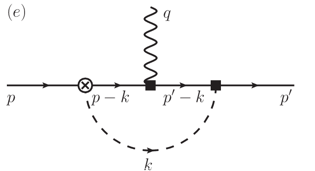
These are tree graphs (a), (b), one-loop graphs starting at $\mathcal{O}(\delta^{2})$ (c)–(h), and one-loop graphs with one insertion from the dimension-two chiral meson–baryon Lagrangian starting at $\mathcal{O}(\delta^{3})$ (i)–(l). To obtain a consistent power counting, the loop diagrams are evaluated using the so-called infrared regularization scheme [18]. In this covariant framework, loop graphs resum an infinite string of higher-order corrections, associated with the $1/m$ insertions in the heavy-baryon propagator. In the following, we will expand these contributions up-to-and-including $\mathcal{O}(\delta^{3})$ . It can be shown that the graphs (g)–(l) do not contribute at this order or cancel each other exactly. For later purpose, it is convenient to decompose the form factor into tree level and loop contributions, $F_{3}=F_{3}^{\rm tree}+F_{3}^{\rm loop}\,$ . After renormalization, the tree level part for the neutron is given by

F_{3,n}^{\rm tree}=-16\,m\,e\,\bar{\theta}_{0}\left[\frac{1}{3}w_{13}^{r}+\frac{48}{F_{0}^{2}F_{\pi}^{2}M_{\eta_{0}}^{2}}V_{3}^{(1)}V_{0}^{(2)}w_{13}\right]\ ,

(14)

where $w_{13}^{r}$ is the finite part of $w^{\prime}_{13}$ . The third-order loop result for the neutron electric dipole form factor follows as

	$\displaystyle F_{3,n}^{\rm loop}\left(q^{2}\right)$	$\displaystyle=$	$\displaystyle\frac{2meV_{0}^{(2)}\bar{\theta}_{0}}{\pi^{2}F_{\pi}^{4}}\Biggl\{(D+F)(b_{D}+b_{F})\biggl[1-\ln\frac{M_{\pi}^{2}}{\mu^{2}}-\sigma_{\pi}\ln\frac{\sigma_{\pi}+1}{\sigma_{\pi}-1}-\frac{\pi}{2}\frac{q^{2}-2M_{\pi}^{2}}{m\sqrt{-q^{2}}}\arctan\frac{\sqrt{-q^{2}}}{2M_{\pi}}\biggr]$
	$\displaystyle-(D$	$\displaystyle-$	$\displaystyle F)(b_{D}-b_{F})\biggl[1-\ln\frac{M_{K}^{2}}{\mu^{2}}-\sigma_{K}\ln\frac{\sigma_{K}+1}{\sigma_{K}-1}-\frac{\pi}{2}\frac{q^{2}-2M_{K}^{2}+4m\Delta m_{\Sigma N}}{m\sqrt{-q^{2}}}\arctan\frac{\sqrt{-q^{2}}}{2M_{K}}\biggr]\Biggr\}\,,$

where, in the space-like region, $q^{2}=-Q^{2}\leq 0$ , $\Delta m_{\Sigma N}=m_{\Sigma}-m$ , which is of order $\delta^{2}$ , and $\sigma_{\pi/K}=\sqrt{1-4M_{\pi/K}^{2}/q^{2}}$ . The second-order result is given by omitting the last term of the pion and kaon part in the expression above. In the limit $q^{2}\to 0$ , one can readily deduce the expression for the electric dipole moment of the neutron,

$\displaystyle d_{n}$	$\displaystyle=$	$\displaystyle d_{n}^{\rm tree}+d_{n}^{\rm loop}~,\qquad d_{n}^{\rm tree}=-8\,e\,\bar{\theta}_{0}\left(\frac{1}{3}w_{13}^{r}+\frac{48}{F_{0}^{2}F_{\pi}^{2}M_{\eta_{0}}^{2}}V_{3}^{(1)}V_{0}^{\left(2\right)}w_{13}\right)~,$
$\displaystyle d_{n}^{\rm loop}$	$\displaystyle=$	$\displaystyle-\frac{e\,V_{0}^{(2)}}{\pi^{2}F_{\pi}^{4}}\bar{\theta}_{0}\Biggl[(D+F)(b_{D}+b_{F})\left(1+\ln{\frac{M_{\pi}^{2}}{\mu^{2}}}-\frac{\pi M_{\pi}}{2m}\right)$	(16)
		$\displaystyle\qquad\qquad\,\,-(D-F)(b_{D}-b_{F})\left(1+\ln\frac{M_{K}^{2}}{\mu^{2}}-\frac{\pi M_{K}}{2m}+\frac{\pi\,\Delta m_{\Sigma N}}{M_{K}}\right)\Biggr]\ .$	(16)

The expression for the tree result was already derived in [7], however we obtain an additional factor of three for diagram (b). Note that we have kept the dependence on the scale of dimensional regularization $\mu$ in the loop expression in order to give an error estimate by varying the scale when performing the numerical evaluation. Dropping all terms besides the chiral logarithms reproduces the result of [9, 7]. The next-to-leading order correction in the pion-loop contribution was also obtained in [19] in a relativistic loop calculation. We have also calculated the corresponding form factor of the proton to achieve an isoscalar/isovector separation in the two-flavor case as discussed below. We refrain from giving the corresponding formulas here [20]. From the neutron and proton form factors one can derive analytic results for the corresponding radii, the one for the neutron reads

	$\displaystyle\left\langle r_{ed}^{2}\right\rangle_{n}=\frac{2eV_{0}^{(2)}}{\pi^{2}F_{\pi}^{4}}\bar{\theta}_{0}\Biggl[(D$	$\displaystyle+$	$\displaystyle F)(b_{D}+b_{F})\left(\frac{m}{M_{\pi}^{2}}-\frac{5\pi}{4M_{\pi}}\right)$
	$\displaystyle-(D$	$\displaystyle-$	$\displaystyle F)(b_{D}-b_{F})\left(\frac{m}{M_{K}^{2}}-\frac{5\pi}{4M_{K}}-\frac{\pi\,m\,\Delta m_{\Sigma N}}{2M_{K}^{3}}\right)\Biggr]~.$		(17)

5. Before showing results, we must fix parameters. We use $D=0.804$ and $F=0.463$ from hyperon $\beta$ -decays [21], $b_{D}=0.066\,{\rm GeV}^{-1}$ and $b_{F}=-0.209\,{\rm GeV}^{-1}$ from the leading-order analysis of the baryon mass splittings, $F_{\pi}=92.4\,$ MeV as well as $V_{0}^{(2)}=-5\cdot 10^{-4}\,$ GeV⁴ and $V_{3}^{(1)}=3.5\cdot 10^{-4}\,$ GeV² from an analysis of $\eta-\eta^{\prime}$ mixing [17]. The same analysis also shows that the correction to $F_{0}/F_{\pi}=1$ is of order $1/N_{c}$ , so that we use $F_{0}=F_{\pi}$ based on the counting rule in Eq. (8).

First, we consider the neutron dipole moment. Following the arguments of [7] based on large- $N_{c}$ counting, the ratio of diagrams (a) and (b) is given by

\Bigg|\frac{d_{n}^{\rm tree(b)}}{d_{n}^{\rm tree(a)}}\Bigg|\simeq\frac{144}{F_{\pi}^{4}M_{\eta_{0}}^{2}}\Big|V_{0}^{(2)}V_{3}^{(1)}\Big|\simeq 0.38\ .

(18)

This ratio will serve for an error estimate of the tree level contribution. Furthermore, the $w_{16}$ -term of the meson–baryon Lagrangian, describing a magnetic coupling to the baryon fields, is similar to the structure proportional to $w^{\prime}_{13}$ / $w_{13}^{r}$ except for the additional $\gamma_{5}$ . However, the coefficient $w_{16}$ is of $\mathcal{O}(N_{c}^{1})$ , whereas $w_{13}^{r}$ is of $\mathcal{O}(N_{c}^{0})$ , which suggests the assumption $|w_{13}^{r}|<|w_{16}|$ . Utilizing the third-order calculation of the baryon electromagnetic form factors [22], we find $w_{16}=0.40\,{\rm GeV}^{-1}$ . Assuming further $|w_{13}^{r}|=|w_{16}|/3$ , we obtain a bound on the dipole moment,

\left|d_{n}^{\rm tree}\right|\simeq\left(2.9\pm 1.1\right)\times 10^{-16}\,\theta_{0}\,e\,\mbox{cm}\ .

(19)

The numerical evaluation of the loop corrections to the electric dipole moment of the neutron is much more straightforward since it does not involve unknown parameters. We find

d_{n}^{\rm loop}=-3.0_{-0.8}^{+1.1}\times 10^{-16}\,\theta_{0}\,e\,\mbox{cm}\ ,

(20)

varying the renormalization scale $\mu$ between $M_{\rho}$ and $m_{\Xi}$ (note the much larger scale variation in [19] that induces an even more pronounced uncertainty). However, it was shown in [23] that the corrections to $b_{D}$ , $b_{F}$ due to fourth-order effects are large, so that the central value for the loop contributions changes to $d_{n}^{\rm loop}=-5.1\times 10^{-16}\,\theta_{0}\,e\,\mbox{cm}.$ Taking this latter value, the loop corrections slightly dominate and we can deduce a lower bound for the theoretical estimate of the electric dipole moment,

\left|d_{n}^{\rm theo}\right|\gtrsim 1.1\times 10^{-16}\,\theta_{0}\,e\,\mbox{cm}\ .

(21)

Together with the experimental upper bound on the electric dipole moment of the neutron, this finally yields

\left|\theta_{0}\right|\lesssim 2.5\times 10^{-10}\ .

(22)

We remark, however, that this bound is very sensitive to cancellations between the tree and loop contributions and based on large- $N_{c}$ arguments, and thus should be considered with caution.

Next, we discuss the loop contribution to the neutron dipole form factor. It is shown in Fig. 2 in units of $e$ times the dimensionless parameter $\theta_{0}$ . The full result including third-order corrections is represented by the solid line, whereas the dashed line contains second-order contributions only. The error bands of both lines are obtained by varying the renormalization scale between $M_{\rho}$ and $m_{\Xi}$ again. The renormalization scale for the central curves has been set to the neutron mass $\mu=m$ . As can be seen from this figure, the relative size of the third-order corrections compared to the leading-order terms is small for reasonable values of $Q^{2}$ . In fact, the change due to the variation of the renormalization scale clearly exceeds the change resulting from third-order corrections. Nevertheless, the slope of the form factor for small values of $Q^{2}$ is altered significantly by the next-to-leading-order corrections, as it is also borne out by evaluating Eq. (17). We find

\langle r^{2}_{ed}\rangle_{n}=-20.4\,\left[1-0.67+\mathcal{O}(\delta^{2})\right]\,\theta_{0}\,e\,{\rm fm}^{2}~,

(23)

and a similar effect is found for the proton. This large correction can be traced back to the additional factors of $\pi$ in the pion loop contribution in Eq. (17). Such factors also appear in the analysis of the radii of the isospin-violating nucleon form factors, see [24]. We also note that the contribution from kaon loops is much smaller than the one from the pions and therefore, the radius is almost entirely of isovector nature.

To compare results from two-flavor lattice QCD at unphysical quark masses with predictions from chiral perturbation theory, it is necessary to perform an extrapolation of the analytic results in the pion mass. To this end, we have to express $\Delta m_{\Sigma N}$ in terms of $M_{\pi}$ , $M_{K}$ and account for the fact that $M_{K}$ itself depends on $M_{\pi}$ . To lowest order this dependence is given by

M_{K}^{2}=\mathring{M}_{K}^{2}+\frac{1}{2}M_{\pi}^{2}\ ,

(24)

where $\mathring{M}_{K}$ denotes the mass of the kaon in the $SU(2)$ chiral limit. Numerically, one has $\mathring{M}_{K}\simeq 0.484\,\mbox{GeV}.$ Special care has to be taken furthermore to relate $\bar{\theta}_{0}$ to $\theta_{0}$ , as Eq. (12) has been derived assuming $m_{u,d}\ll m_{s}$ , as well as a certain hierarchy of terms relying on the numerical value of $V_{0}^{(2)}$ . Giving up those assumptions changes the relation between $\bar{\theta}_{0}$ and $\theta_{0}$ to

\bar{\theta}_{0}=\left(1+\frac{4V_{0}^{(2)}}{F_{\pi}^{2}}\frac{4M_{K}^{2}-M_{\pi}^{2}}{M_{\pi}^{2}\left(2M_{K}^{2}-M_{\pi}^{2}\right)}\right)^{-1}\,\theta_{0}\ .

(25)

In Fig. 3 we show the resulting pion (quark) mass dependence of the loop contribution to the electric dipole moment in comparison to the available data points from two-flavor lattice QCD [4]. It is interesting to see that the third-order calculation reproduces the trend of the lattice data (the order of magnitude and the global sign) even without the unknown tree contribution. However, only below pion masses of the order of 500 MeV the third-order corrections are sufficiently small for a stable chiral extrapolation.

6. Finally we consider the matching of our three-flavor results to the two-flavor representation. This not only allows to extend the findings of [10] to higher order, but also gives an explicit representation for some of the LECs appearing in that paper. Such matching relations between three- and two-flavor versions of chiral perturbation theory have been studied extensively in the meson sector (see the most recent comprehensive results [25, 26] and references therein), and also first results for the meson–baryon sector exist [27, 28].

The leading-order $SU(2)$ formulas for the electric dipole moment of the nucleon have been worked out in [10], within the framework of heavy-baryon chiral perturbation theory. The authors employ a decomposition of the electric dipole form factor of the nucleon according to

J_{ed}^{\nu}=-\frac{1}{2m}\sigma^{\mu\nu}q_{\mu}\gamma_{5}\left(F_{3}^{(0)}(q^{2})+F_{3}^{(1)}(q^{2})\tau_{3}\right)\ ,

(26)

where $F_{3}^{(0)}(q^{2})$ is the isoscalar and $F_{3}^{(1)}(q^{2})$ is the isovector part of the electric dipole form factor. The relations between the corresponding isoscalar and isovector electric dipole moments $d_{0/1}$ and those of proton and neutron are given by

d_{0/1}=\frac{1}{2}(d_{p}\pm d_{n})\ .

(27)

By matching our $SU(3)$ result to the two-flavor theory, we can extend the expressions given in [10] by one order in the chiral expansion,

d_{0}=\tilde{d}_{0}+\frac{eg_{A}\bar{g}_{\pi NN}}{8\pi^{2}F_{\pi}}\left(-\frac{3\pi}{4}\frac{M_{\pi}}{m}\right)~,\qquad d_{1}=\tilde{d}_{1}+\frac{eg_{A}\bar{g}_{\pi NN}}{8\pi^{2}F_{\pi}}\left(1+\ln\frac{M_{\pi}^{2}}{\mu^{2}}-\frac{5\pi}{4}\frac{M_{\pi}}{m}\right)~,

(28)

where the $\tilde{d}_{0/1}$ parameterize the short-distance physics that now includes kaon, $\eta_{8}$ , and $\eta_{0}$ loops. Explicitly, the matching relations for these two constants read

$\displaystyle\tilde{d}_{0/1}$	$\displaystyle=$	$\displaystyle\frac{1}{2}\big(\tilde{d}_{p}^{\rm tree}+\tilde{d}_{p}^{\rm loop}\big)\pm\frac{1}{2}\big(\tilde{d}_{n}^{\rm tree}+\tilde{d}_{n}^{\rm loop}\big)+\mathcal{O}\big(M_{K}^{2},M_{\eta_{0}}^{2}\big)~,$
$\displaystyle\tilde{d}_{p}^{\rm tree}$	$\displaystyle=$	$\displaystyle-\frac{\tilde{d}_{n}^{\rm tree}}{2}+12\,e\,\bar{\theta}_{0}\bigg(\frac{w_{14}^{r}}{3}+\frac{48V_{3}^{(1)}V_{0}^{(2)}}{F_{0}^{2}F_{\pi}^{2}M_{\eta_{0}}^{2}}w_{14}\bigg)~,\quad\tilde{d}_{n}^{\rm tree}=-8\,e\,\bar{\theta}_{0}\bigg(\frac{w_{13}^{r}}{3}+\frac{48V_{3}^{(1)}V_{0}^{\left(2\right)}}{F_{0}^{2}F_{\pi}^{2}M_{\eta_{0}}^{2}}w_{13}\bigg)~,$
$\displaystyle\tilde{d}_{p}^{\rm loop}$	$\displaystyle=$	$\displaystyle\frac{\tilde{d}_{n}^{\rm loop}}{2}+\frac{e\,V_{0}^{(2)}}{\pi^{2}F_{\pi}^{4}}\bar{\theta}_{0}\Biggl[\frac{1}{6}(D+3F)(b_{D}+3b_{F})\left(1+\ln\frac{M_{K}^{2}}{\mu^{2}}-\frac{3\pi M_{K}}{2m}-\frac{4}{3}\pi(b_{D}+3b_{F})M_{K}\right)$
		$\displaystyle-\bigg(\frac{3}{2}(D-F)(b_{D}-b_{F})+\frac{(D-3F)(b_{D}-3b_{F})}{3\sqrt{3}}\bigg)\frac{\pi M_{K}}{m}$
		$\displaystyle-(2D+3\lambda)\left(2b_{D}+3b_{0}+6\sqrt{3}w^{\prime}_{10}\right)\frac{\pi M_{\eta_{0}}}{6\sqrt{3}m}\frac{F_{\pi}^{2}}{F_{0}^{2}}\Biggr]~,$
$\displaystyle\tilde{d}_{n}^{\rm loop}$	$\displaystyle=$	$\displaystyle\frac{e\,V_{0}^{(2)}}{\pi^{2}F_{\pi}^{4}}\bar{\theta}_{0}\Biggl[(D-F)(b_{D}-b_{F})\left(1+\ln\frac{M_{K}^{2}}{\mu^{2}}-\frac{\pi M_{K}}{2m}+4\pi(b_{D}-b_{F})M_{K}\right)\Biggr]~,$	(29)

where we have used the $SU(2)$ chiral limit relation $M_{\eta_{8}}=2M_{K}/\sqrt{3}$ . The new terms in the $SU(2)$ expressions Eq. (28) are the ones linear in the pion mass. We note that the corrections $\sim M_{\pi}$ are again sizeable. Furthermore, it was argued in [10] based on dimensional analysis that the CP-violating pion–nucleon coupling $\bar{g}_{\pi NN}$ has to be of order

\bar{g}_{\pi NN}=\mathcal{O}\bigg(\frac{\theta_{0}M_{\pi}^{2}}{m\,F_{\pi}}\bigg)\ .

(30)

The previous results allow us to obtain a matching relation for $\bar{g}_{\pi NN}$ . Utilizing the standard matching relation for the two- and three-flavor axial couplings, $g_{A}=D+F+\mathcal{O}(\delta^{2})$ , we obtain for $\bar{g}_{\pi NN}$

\bar{g}_{\pi NN}=\frac{\theta_{0}M_{\pi}^{2}}{F_{\pi}}\left(b_{D}+b_{F}\right)+\mathcal{O}\left(\delta^{4}\right)\,,

(31)

which numerically yields $\bar{g}_{\pi NN}=-0.03[-0.05]\,\theta_{0}$ , where the number in the brackets refers to the values of $b_{D/F}$ from [23]. This confirms the dimensional estimate equation (30) and reproduces the result originally obtained in [8]. However, our representation in terms of symmetry-breaking LECs only is certainly more compact and can be systematically improved by going to yet higher orders in the chiral expansion.

7. In this Letter, we have analyzed the neutron (and proton) electric dipole form factor and its moment in the framework of covariant $U(3)_{L}\times U(3)_{R}$ baryon chiral perturbation theory, extending earlier calculations by one order in the power counting. The latter includes the expansion of QCD in the number of colors. While the third-order corrections to the neutron electric dipole moment are small at the physical pion mass, their contribution makes the trend of the quark-mass expansion agree with the existing data from full lattice QCD, although those still employ pion masses too high for a safe chiral extrapolation. More lattice data at smaller pion masses will allow one to analyze strong CP violation as encoded in the neutron electric dipole moment in more detail. From comparison with experimental limits, we have given an upper bound on the vacuum angle. The electric dipole radius, given entirely by chiral loops, receives a large correction at next-to-leading order. Finally, we have also given matching relations for our three-flavor representation to the $SU(2)$ case.

We would like to thank Jambul Gegelia for useful discussions. We acknowledge the support of the European Community Research Infrastructure Integrating Activity “Study of Strongly Interacting Matter” (acronym HadronPhysics2, Grant Agreement n. 227431) under the Seventh Framework Programme of the EU. Work supported in part by DFG (SFB/TR 16, “Subnuclear Structure of Matter”), by the Helmholtz Association through funds provided to the virtual institute “Spin and strong QCD” (VH-VI-231), by BMBF “Strong interaction studies for FAIR” (grant 06BN9006), and by the Bonn-Cologne Graduate School of Physics and Astronomy.

References

[1] C. A. Baker et al., Phys. Rev. Lett. 97 (2006) 131801 [arXiv:hep-ex/0602020].
[2] S. K. Lamoreaux and R. Golub, J. Phys. G 36 (2009) 104002.
[3] F. Berruto, T. Blum, K. Orginos and A. Soni, Phys. Rev. D 73 (2006) 054509 [arXiv:hep-lat/0512004].
[4] E. Shintani, S. Aoki and Y. Kuramashi, Phys. Rev. D 78 (2008) 014503 [arXiv:0803.0797 [hep-lat]].
[5] R. Horsley et al., arXiv:0808.1428 [hep-lat].
[6] S. D. Thomas, Phys. Rev. D 51 (1995) 3955 [arXiv:hep-ph/9402237].
[7] B. Borasoy, Phys. Rev. D 61 (2000) 114017 [arXiv:hep-ph/0004011].
[8] R. J. Crewther, P. Di Vecchia, G. Veneziano and E. Witten, Phys. Lett. B 88 (1979) 123 [Erratum-ibid. B 91 (1980) 487].
[9] A. Pich and E. de Rafael, Nucl. Phys. B 367 (1991) 313.
[10] W. H. Hockings and U. van Kolck, Phys. Lett. B 605 (2005) 273 [arXiv:nucl-th/0508012].
[11] D. O’Connell and M. J. Savage, Phys. Lett. B 633 (2006) 319 [arXiv:hep-lat/0508009].
[12] J. W. Chen, D. O’Connell and A. Walker-Loud, JHEP 0904 (2009) 090 [arXiv:0706.0035 [hep-lat]].
[13] J. Gasser and H. Leutwyler, Nucl. Phys. B 250 (1985) 465.
[14] H. Leutwyler, Phys. Lett. B 374 (1996) 163 [arXiv:hep-ph/9601234].
[15] P. Herrera-Siklódy, J. I. Latorre, P. Pascual and J. Taron, Nucl. Phys. B 497 (1997) 345 [arXiv:hep-ph/9610549].
[16] R. Kaiser and H. Leutwyler, Eur. Phys. J. C 17 (2000) 623 [arXiv:hep-ph/0007101].
[17] P. Herrera-Siklódy, J. I. Latorre, P. Pascual and J. Taron, Phys. Lett. B 419 (1998) 326 [arXiv:hep-ph/9710268].
[18] T. Becher and H. Leutwyler, Eur. Phys. J. C 9 (1999) 643 [arXiv:hep-ph/9901384].
[19] S. Narison, Phys. Lett. B 666 (2008) 455 [arXiv:0806.2618 [hep-ph]].
[20] K. Ottnad, Diploma thesis, University of Bonn (2009).
[21] H.-W. Siebert, in: H. Abele and D. Mund (eds.), arXiv:hep-ph/0312124.
[22] B. Kubis and U.-G. Meißner, Eur. Phys. J. C 18 (2001) 747 [arXiv:hep-ph/0010283].
[23] B. Borasoy and U.-G. Meißner, Annals Phys. 254 (1997) 192 [arXiv:hep-ph/9607432].
[24] B. Kubis and R. Lewis, Phys. Rev. C 74 (2006) 015204 [arXiv:nucl-th/0605006].
[25] J. Gasser, C. Haefeli, M. A. Ivanov and M. Schmid, Phys. Lett. B 652 (2007) 21 [arXiv:0706.0955 [hep-ph]].
[26] J. Gasser, C. Haefeli, M. A. Ivanov and M. Schmid, Phys. Lett. B 675 (2009) 49 [arXiv:0903.0801 [hep-ph]].
[27] M. Frink and U.-G. Meißner, JHEP 0407 (2004) 028 [arXiv:hep-lat/0404018].
[28] M. Mai, P. C. Bruns, B. Kubis and U.-G. Meißner, Phys. Rev. D 80 (2009) 094006 [arXiv:0905.2810 [hep-ph]].