SINP/TNP/2009/25
Correlated enhancements in , of muon, and lepton flavor violating decays with two -parity violating couplings
Gautam Bhattacharyya 1, Kalyan Brata Chatterjee 1, and Soumitra Nandi 2
1) Saha Institute of Nuclear Physics,
1/AF Bidhan Nagar, Kolkata 700064, India
2) Dipartimento di Fisica Teorica, Univ. di Torino and INFN,
Sezione di Torino, I-10125 Torino, Italy
Abstract
With just two -parity violating couplings, and , we correlate several channels, namely, (), , and some lepton flavor violating decays. For and for a common superpartner mass of 300 GeV, which explain the recently observed excesses in the above decay channels, we predict the following -parity violating contributions: , , , and . We exhibit our results through observable versus observable correlation plots.
PACS Nos: 12.60.Jv, 13.35.Dx
Key Words: -parity violation, Lepton flavor violation
1 Motivation
While all attention is now focused on the Large Hadron Collider (LHC) as a possible gold mine of physics beyond the standard model (SM), one should not lose sight of other territories rich with new physics, e.g., lepton flavor violating (LFV) rare decays, which could provide complementary information. Ever since neutrino flavor mixing was established, interests for observing flavor violation in charged lepton decays have boomed. While in the neutrino sector flavor violation could be rather large (maximal between and ), in the charged lepton decays there is no sign of flavor violation as yet. The SM contributions to charged LFV decays are quite small, orders of magnitude below the current experimental sensitivity, due to the smallness of neutrino mass. Hence, any observation of LFV processes in the charged lepton sector, which are being probed with ever increasing sensitivity, would unambiguously point to non-standard interactions. Indeed, such indirect observations taken in isolation may not imply much on the exact nature of new physics. But a study of possible correlations of its effects on different independently measured charged LFV observables might provide a powerful cross-check and lead to identification of new physics through LHC/LFV synergy. In this paper, we consider -parity violating (RPV) supersymmetry [1] and perform a correlation analysis of its numerical impact on different LFV decays. We also study at tandem the RPV contribution to , an observable which continues to provide a room for new physics despite significantly improved theoretical and experimental accuracies.
-parity is a discrete symmetry, which is defined as , where , , and are the baryon number, lepton number and spin of a particle, respectively. is for all SM particles and for their superpartners. The usual assumption of and conservation in supersymmetric models are not supported by any deep underlying principle. The -violating -type superpotential is written as , where stands for SU(2) doublet lepton superfields, for SU(2) doublet quark superfields, for SU(2) singlet down-type quark superfields, and are generation indices. There are 27 such couplings, on each of which and also on many of their combinations exist strong constraints [2, 3]. We select only two of them, namely and , and consider only them to be large and the rest to be either vanishing or negligibly small.
Why and ? It has been observed that these two couplings (each with a magnitude of and for superparticle masses around 300 GeV) can justify the recently observed large branching ratios that the SM cannot explain [4]. On top of that, if we turn on even a small , then together with , one can also explain the large phase in – mixing [4, 5]. Turning our attention to the neutrino sector, we recall that generation of neutrino masses and mixing by -type couplings usually require a specific combination of indices, namely, the product couplings [6]. But if we take and (together with as the only non-vanishing and large RPV couplings, a phenomenologically acceptable pattern of neutrino masses and mixing emerge at two-loop level [7]. To sum up, we consider four non-vanishing RPV couplings: two of them and large () and relevant for the present analysis, the other two and (from charged-current universality [2]) not to be used in the present analysis but implicitly present to justify our choices of and through the correlated phenomena mentioned above. Now, motivated by the observation of maximal mixing between and , we make a further assumption . Keeping all these in mind, we outline our agenda as follows: consider and as the only two relevant RPV couplings (the other two, viz. and , optional and small), assume them to be real, set their magnitudes equal and just enough to explain the anomaly, predict its effect on , and estimate its numerical impact on different LFV decays (, , , ). For simplicity, we assume all squark and slepton masses to be degenerate, and denote the common mass by . We derive various one-loop effective flavor violating vertices, which we have often referred to as form-factors. We display their exact as well as approximate expressions. While for numerical plots we use the exact formulae, the approximate expressions serve to provide an intuitive feel of the numerical impact.
2 and the anomaly
The branching fraction of the leptonic decay () is given by
| (1) |
where is the lifetime of . The decay constant is defined as , where is the momentum of . The branching ratio has a helicity suppression factor characterized by on account of a spin-zero particle decaying into two spin-half particles. Monte-Carlo simulations of QCD on lattice predict MeV [8]. The experimental average is somewhat higher: MeV [9, 10, 11]. The enhancements are in the muon channel, in the tau channel, and on average. On the other hand, the lattice estimate and the experimentally obtained value for seem to be in perfect agreement around 206 MeV [8]. The latter suggests that the discrepancy in may very well be influenced by new physics contributing in a flavor specific way to decay. Note that in the SM proceeds at tree level and it is Cabibbo-allowed. Hence, loop suppressed new physics is an unlikely candidate to account for the discrepancy. Leptoquark or charged Higgs interactions have been advocated in this context as they provide new tree amplitudes for the above decay [12]. Our candidate is supersymmetric RPV interaction and our chosen couplings, and , contribute to via -exchanged tree graphs [4]. The net contribution to the channel can be obtained by replacing in Eq. (1) by
| (2) |
For , we must do the replacements in Eq. (2).
3 Anomalous magnetic moment of the muon
The effective vertex of photon with any charged fermion is given by
| (3) |
The muon magnetic moment for is given by . At tree level, and . Quantum correction yields , while remains unity at all order due to charge conservation. Since , it follows that . As per current estimation [13], the room for new physics is given by
| (4) |

The coupling induces a contribution to , which proceeds through the diagrams in Fig. 1. The quarks and squarks inside the loop have been labeled by generic symbols and respectively, which can take two sets: and . The loop integrals would depend on and . As mentioned earlier and assumed throughout our analysis, . We obtain
| (5) | |||||
The -functions used throughout our analysis are given by
| (6) |
4 decay
The decay proceeds through photon and penguins (Fig. 2) and box graph (Fig. 3). We consider each of them below. Here flavor violation is induced by and via loops with quarks and squarks in internal lines.
4.1 Photon penguin

The amplitude of the photon exchanged diagrams for decay can be written as
| (7) |
where is the photon momentum. The form-factors and are induced by the flavor-changing couplings. Each penguin diagram will have a quark () and a squark () inside the loop. There are two such sets: and . We obtain
| (8) | |||||
The magnetic form-factor is given by
| (9) | |||||
4.2 -boson penguin
The -mediated penguin amplitude for the process is given by
| (10) |
The boson couplings with the left- and right-chiral fermions are given by
| (11) |
The -induced contribution to the form-factor proceeds through two sets of penguins: and , yielding
| (12) |
4.3 Box contribution
The and couplings also induce a box graph for with internal quark and squark lines. Again, two sets of box diagrams contribute and . The amplitude is given by

| (13) |
For the sake of convenience, we normalize with a prefactor , though no gauge interaction is actually involved:
| (14) |
4.4 The branching ratio
The total decay amplitude of this process is the sum of the penguin and box contributions, given by . The branching ratio of is given in terms of the different form-factors [14]:
| (15) | |||||
where is the total decay width of . Our form-factors () are all real. The expressions of and are given by,
| (16) |
5 Radiative decay

We have shown in Fig. 4 how together with drive the magnetic transition . The amplitude for this transition is given by
| (17) |
where is the photon polarization. The expression for can be found in Eq. (9). In the amplitude we have neglected a similar term proportional to . The branching ratio for this radiative decay mode is given by (neglecting any -dependent term)
| (18) |
6 Semileptonic lepton flavor violating decay :
The semileptonic decay with decay is mediated by a -penguin and a box graph, as shown in Figs. (5a) and (5b), respectively. Photon penguin cannot contribute as it cannot provide the axial current for the quarks to condense to a meson.

The -boson mediated penguin amplitude for is given by
| (19) |
where and are given in Eq. (11). The relevant for the formation of and are and . The form factor is already given in Eq. (12).
The couplings and also induce through box graphs. Because of the specific -indices, can only be . The box graph contains two fermion lines and two scalar lines. There are two types of box diagrams: (i) the fermions are the same ( quark), but the scalars are different ( and ); (ii) the scalars are same (), but the fermions are different ( and ). The sum of box amplitudes is given by,
| (20) |
The form-factor is given by
| (21) |
where has already been expressed in Eq. (14), while is given by
| (22) |
Using Eqs. (19-22) we obtain the branching ratio,
| (23) |
The decay constants involving and are given by
| (24) |
The numerical values of the involved parameters are given by [15, 9];
| (25) |
7 Results
In Table 1 we have displayed the present experimental status of different branching ratios of our concern.
| Decay modes | Branching fractions |
|---|---|
Existing limits on : We reiterate that all our processes are driven by and . The existing limits on them depend on . As mentioned before, throughout our analysis we have assumed a common sparticle mass of 300 GeV. The best upper limit on comes from , and the limit is 0.3 at 90% C.L. [3, 18]11 1 It is interesting to observe that the 2 upper limit obtained in [18] with is not much different from the latest update at 2 for GeV using [3]. In spite of a significant reduction of the error on (over a period of 14 years), the 2 upper limit on remained more or less the same because the central value gradually moved towards unity.. On the other hand, the best upper limit on arises from , the limit being 0.9 at 90% C.L. [3].
Our parameters: Recall that maximal mixing between and motivated us to assume . For showing numerical correlations through different plots, we scan in the range , but keep fixed at 300 GeV. Also, the band width in each plot is a consequence of varying by 2 around its central value, i.e. in the range MeV. As we go from left to right in each band the value of increases. The minimum values of consistent with 2 lower limits of and are 0.3 and 0.4, respectively, which correspond to (the 2 upper limit of) MeV.
Contribution to : Following Eq. (5), we obtain
| (26) |
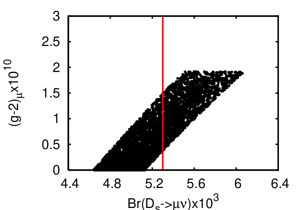
In Fig. 6, we have plotted the correlation between contribution to along one axis and the branching ratio of along the other. We note here that the -parity conserving contribution to can be sizable too for large . In fact, an approximate expression for can be found in [19] as
| (27) |
LFV decays: The approximate (yet, to a very good accuracy) expressions of the LFV form-factors with their explicit dependence on and (the other parameters are all known) are as follows:
| (28) | |||
Since each box has four -vertices, and have both quartic sensitivity to , while the penguin form-factors have quadratic dependence on . Using the expressions in Eq. (28), we calculate the branching ratios to a very good approximation as
| (29) | |||||
| (30) | |||||
| (31) | |||||
| (32) |
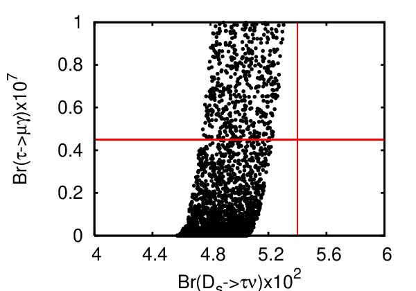
In Eq. (29), the first term within the square bracket is the pure penguin contribution, the second term represents interference between penguin and box graphs, while the last term is the pure box contribution. As explained before, the dependence is different for different terms. Also, by comparing Eq. (30) with Eq. (29), we observe that for the same choices of and the prediction of is one order of magnitude enhanced compared to . This happens primarily because the latter is a 3-body decay which involves more suppression factors which cannot compensate the fact that . Figs. 7a and 7b capture the numerical correlations. We observe that the region allowed at 2 by overshoots the 90% C.L. upper limit of the branching ratio of . Obviously, the same thing happens for . However, we should keep in mind that the branching ratio of ( in the present context) has not only an experimental uncertainty, but also inherits a theoretical uncertainty from . Even by mild stretching of one or both of these uncertainties beyond 2, it is possible to accommodate both and .

|
|
New Limit: The upper limit on branching ratio (see Table 1) restricts . Our limit is stronger than before and, without any need of the assumption , should be interpreted as
| (33) |
Since the branching ratios require at 2 (or 90% C.L.), to avoid conflict with Eq. (33) we need to stretch the present limits, as already mentioned. If we fix , the prediction for the branching ratio of is , which is roughly a factor of 3 below the current sensitivity, but still very much within the reach of the super factory with 75 projected luminosity. If, however, remains elusive even at super, then as per our prediction, is not going to be observed either.
The branching ratio of , expressed in Eq. (23), contains contributions from box (the part) and penguin (the part). The box contribution is significantly more dominant than the penguin. We display the approximate numerical values of the branching ratios for and in Eqs. (31) and (32), respectively. The dependences on and are similar as both processes involve similar box graphs. As expected, these modes are not as constraining as . If we put , the branching ratios for the and modes are predicted to be around , i.e. two orders of magnitude below the present sensitivity, but within the accuracy expected to be reached at the super factory with 75 luminosity. Again, a positive signal at Super necessarily requires an observation of at the current sensitivity. The numerical correlations of and decay modes with the branching fraction have been plotted in Fig. 8.

|

|
8 Comparison with previous works and conclusions
We divide this section in three parts: (i) we briefly mention about the existing studies on -parity conserving supersymmetric contribution to LFV decays, (ii) remark on the previous works on -parity violating contributions to lepton flavor violation, and finally (iii) highlight the new things that we have done in this work.
(i) LFV decays have been analyzed in supersymmetric scenarios with conserved -parity but with different sets of supersymmetry breaking parameters. In a class of scenarios where minimal supersymmetry is augmented by three right-handed neutrino superfields for generating neutrino masses via see-saw mechanism, it has been shown [14, 20] that large neutrino Yukawa couplings induce large flavor violation in the slepton sector which is ultimately transmitted to the LFV observables. The general conclusion is that light supersymmetry ( GeV) is disfavored. Large LFV branching ratios (with large ) can be obtained when light neutrino masses are hierarchical. In general, is the most sensitive LFV channel, but to explore the Higgs sector and channels are more effective. It has been shown that in a general unconstrained minimal supersymmetric framework [21], for low , the branching ratio in the channel is and in the channel less than . On the other hand, for large and for small pseudo-scalar mass (), the Higgs mediated contributions are extremely dominant. In the latter case, indeed with strong fine-tuning of parameters, is enhanced to and to even larger values. In supersymmetric models embedded in minimal SO(10) group [22], the LFV branching ratios are, however, several orders of magnitude below the present experimental sensitivities.
(ii) RPV induced LFV processes have been studied in the past in different contexts [23]. Except , all other LFV processes considered there proceed at tree level with appropriately chosen RPV couplings. The choices of such couplings are, in general, different in different processes. Their primary intentions were to put upper limits on different single and product couplings by confronting LFV observables with experimental results.
(iii) What are the new things that we have done in this paper? We made an economical choice of RPV couplings ( and only), motivated primarily by their ability to explain the large () branching ratios. We set these two couplings equal, a choice inspired by maximal - mixing. We have kept the sparticle mass fixed at 300 GeV. Explanation of branching ratios require at 90% C.L. On the other hand, with an upper limit of on its branching ratio at 90% C.L. offers the most sensitive LFV probe of the RPV dynamics, and sets an improved upper limit at 90% C.L. Enhanced theoretical and experimental accuracies in the channels might eventually release the tension between the apparently conflicting requirements. Putting , we obtain , and . The correlation plots capture the underlying dynamics. To sum up, instead of considering just one experimental observation at a time, be it an anomaly or an excess vis-à-vis the SM expectation, providing a raison d’être for one set of new interactions, we have studied the possibility of correlated enhancements in a variety of LFV channels using just two RPV couplings. We demonstrated our results through ‘observable versus observable’ plots.
Acknowledgments: GB thanks the CERN Theory Division for hospitality and acknowledges a partial support through the project No. 2007/37/9/BRNS of BRNS (DAE), India. SN’s work is supported by a European Community’s Marie-Curie Research Training Network under contract MRTN-CT-2006-035505 ‘Tools and Precision Calculations for Physics Discoveries at Colliders’.
References
- [1] G. R. Farrar and P. Fayet, Phys. Lett. B 76 (1978) 575; S. Weinberg, Phys. Rev. D 26 (1982) 287; N. Sakai and T. Yanagida, Nucl. Phys. B 197 (1982) 533; C. S. Aulakh and R. N. Mohapatra, Phys. Lett. B 119 (1982) 136.
- [2] For reviews see, G. Bhattacharyya, Nucl. Phys. Proc. Suppl. 52A (1997) 83 [arXiv:hep-ph/9608415]; G. Bhattacharyya, arXiv:hep-ph/9709395; H. K. Dreiner, arXiv:hep-ph/9707435; M. Chemtob, Prog. Part. Nucl. Phys. 54 (2005) 71 [arXiv:hep-ph/0406029]; R. Barbier et al., Phys. Rept. 420 (2005) 1 [arXiv:hep-ph/0406039].
- [3] For a very recent update on single RPV couplings, see Y. Kao and T. Takeuchi, arXiv:0910.4980 [hep-ph].
- [4] A. Kundu and S. Nandi, Phys. Rev. D 78 (2008) 015009 [arXiv:0803.1898 [hep-ph]]. A possible contribution from product couplings has also been mentioned in A. G. Akeroyd and S. Recksiegel, Phys. Lett. B 554 (2003) 38 [arXiv:hep-ph/0210376].
- [5] S. Nandi and J. P. Saha, Phys. Rev. D 74 (2006) 095007 [arXiv:hep-ph/0608341].
- [6] G. Bhattacharyya, H. V. Klapdor-Kleingrothaus and H. Pas, Phys. Lett. B 463 (1999) 77 [arXiv:hep-ph/9907432]; S. Rakshit, G. Bhattacharyya and A. Raychaudhuri, Phys. Rev. D 59 (1999) 091701 [arXiv:hep-ph/9811500]. A. Abada, G. Bhattacharyya and M. Losada, Phys. Rev. D 66 (2002) 071701 [arXiv:hep-ph/0208009]. This is only a partial list. See [2] for other references on neutrino mass generation by RPV couplings.
- [7] P. Dey, A. Kundu, B. Mukhopadhyaya and S. Nandi, JHEP 0812 (2008) 100 [arXiv:0808.1523 [hep-ph]].
- [8] T. Onogi, arXiv:0906.5194 [hep-ph].
- [9] C. Amsler et al. [Particle Data Group], Phys. Lett. B 667 (2008) 1, and http://pdg.lbl.gov for 2009 partial update.
- [10] B. I. Eisenstein et al. [CLEO Collaboration], Phys. Rev. D 78 (2008) 052003 [arXiv:0806.2112 [hep-ex]]. An updated CLEO result can be found in arXiv:0910.3602. We thank Sheldon Stone for pointing this out to us.
- [11] K. Abe et al. [Belle Collaboration], Phys. Rev. Lett. 100 (2008) 241801 [arXiv:0709.1340 [hep-ex]].
- [12] B. A. Dobrescu and A. S. Kronfeld, Phys. Rev. Lett. 100 (2008) 241802 [arXiv:0803.0512 [hep-ph]]; R. Benbrik and C. H. Chen, Phys. Lett. B 672 (2009) 172 [arXiv:0807.2373 [hep-ph]]; I. Dorsner, S. Fajfer, J. F. Kamenik and N. Kosnik, arXiv:0906.5585 [hep-ph].
- [13] F. Jegerlehner and A. Nyffeler, Phys. Rept. 477 (2009) 1 [arXiv:0902.3360 [hep-ph]]. For a recent update, see J. Prades, arXiv:0909.2546 [hep-ph].
- [14] E. Arganda and M. J. Herrero, Phys. Rev. D 73 (2006) 055003 [arXiv:hep-ph/0510405]; J. Hisano, T. Moroi, K. Tobe and M. Yamaguchi, Phys. Rev. D 53 (1996) 2442 [arXiv:hep-ph/9510309].
- [15] T. Feldmann and P. Kroll, Eur. Phys. J. C 5 (1998) 327 [arXiv:hep-ph/9711231].
- [16] S. Banerjee, Nucl. Phys. Proc. Suppl. 169 (2007) 199 [arXiv:hep-ex/0702017].
- [17] M. Bona et al., “SuperB: A High-Luminosity Asymmetric Super Flavor Factory. Conceptual Design Report,” arXiv:0709.0451 [hep-ex].
- [18] G. Bhattacharyya and D. Choudhury, Mod. Phys. Lett. A 10 (1995) 1699 [arXiv:hep-ph/9503263].
- [19] M. S. Carena, G. F. Giudice and C. E. M. Wagner, Phys. Lett. B 390 (1997) 234 [arXiv:hep-ph/9610233]. See also (a partial list), T. Moroi, Phys. Rev. D 53 (1996) 6565 [Erratum-ibid. D 56 (1997) 4424] [arXiv:hep-ph/9512396]; U. Chattopadhyay and P. Nath, Phys. Rev. D 53 (1996) 1648 [arXiv:hep-ph/9507386]; R. Barbieri and L. Maiani, Phys. Lett. B 117 (1982) 203.
- [20] E. Arganda, M. J. Herrero and J. Portoles, JHEP 0806 (2008) 079 [arXiv:0803.2039 [hep-ph]]; K. S. Babu and C. Kolda, Phys. Rev. Lett. 89 (2002) 241802 [arXiv:hep-ph/0206310].
- [21] A. Brignole and A. Rossi, Nucl. Phys. B 701 (2004) 3 [arXiv:hep-ph/0404211].
- [22] T. Fukuyama, A. Ilakovac and T. Kikuchi, Eur. Phys. J. C 56 (2008) 125 [arXiv:hep-ph/0506295];
- [23] H. K. Dreiner, M. Kramer and B. O’Leary, Phys. Rev. D 75 (2007) 114016 [arXiv:hep-ph/0612278]; J. Cao, L. Wu and J. M. Yang, arXiv:0908.4556 [hep-ph]; W. j. Li, Y. d. Yang and X. d. Zhang, Phys. Rev. D 73 (2006) 073005 [arXiv:hep-ph/0511273]; A. Gemintern, S. Bar-Shalom, G. Eilam and F. Krauss, Phys. Rev. D 67 (2003) 115012 [arXiv:hep-ph/0302186]; K. m. Cheung and O. C. W. Kong, Phys. Rev. D 64 (2001) 095007 [arXiv:hep-ph/0101347]; A. de Gouvea, S. Lola and K. Tobe, Phys. Rev. D 63 (2001) 035004 [arXiv:hep-ph/0008085]; J. E. Kim, P. Ko and D. G. Lee, Phys. Rev. D 56 (1997) 100 [arXiv:hep-ph/9701381]; D. Choudhury and P. Roy, Phys. Lett. B 378 (1996) 153 [arXiv:hep-ph/9603363].